
1 Introduction
In July 2012, the CMS and Atlas collaborations working at the Large Hadron Collider (LHC) at CERN in Geneva, Switzerland jointly announced [Reference Aad, Abajyan and Abbott1],[Reference Chatrchyan, Khachatryan and Sirunyan2] the detection of a scalar boson of mass roughly 125 GeV decaying into two photons and exhibiting the properties of the Higgs boson, the particle remnant of the electroweak symmetry-breaking mechanism of the Standard Model (SM) of particle physics. For their theoretical work describing this mechanism, P. Higgs and F. Englert were jointly awarded the 2013 Nobel Prize in Physics. This prize was really all about the role of symmetry, its form and its realization, in the electroweak interactions. Symmetry has also played a crucial role in the development of the theory of strong interactions, Quantum Chromodynamics (QCD), the other component of the Standard Model. In fact, one might argue that the deeper understanding of symmetry in many ways underlies much of the physics of the past century. In this Element we discuss the role symmetry played leading to the construction of the SM. The treatment makes no real attempt to strictly follow the chronological development of the SM. However, we try to indicate some of the important hurdles encountered along the way and how they were overcome. In addition, this approach gives us the opportunity to introduce in a natural fashion some of the basic concepts that underlie the Standard Model. We then briefly discuss some of the model’s successes and limitations as well as some open questions that appear to require extensions beyond the model.
The modern view of the role of symmetry originated with Albert Einstein, whose general theory of relativity [Reference Einstein3],[Reference Einstein4] related gravitational interactions to the principle of general coordinate invariance. The use of a symmetry principle as the primary feature of nature that constrains and even dictates the allowable dynamical laws lies at the heart of the Standard Model. The Standard Model is designed to describe the strong, weak and electromagnetic interactions while treating gravity as a classical (flat) background. Thus it must respect the principles of special relativity. In addition, the dynamics needs to conform to the postulates of quantum theory. Since special relativity allows for particle pair production, any formulation must be able to account for arbitrary and varying numbers of particles. The only consistent way to achieve this is using a relativistic quantum field theory, with the textbook of Peskin and Schroeder [Reference Peskin and Schroeder5] being one commonly used for reference. Here the particle modes arise as excitations of operator quantum fields
 , labeled by the space-time point
 and an index
 that distinguishes the various fields. (Appendix A.1 details the notations and convention employed.) The dynamics is encoded within the action functional
 (1.1)
(1.1)
where the local Lagrangian density
 is a function of the quantum fields and their space-time derivatives. This Lagrangian will also depend on various parameters. To fully define the theory, these parameters need to be fixed by certain normalization conditions. Using the Lagrangian, one extracts the various Feynman rules that can be employed in perturbative calculations. Some of the radiative corrections that arise from Feynman graphs containing closed loops can be included by defining scale-dependent (running) couplings to replace the couplings appearing in the Lagrangian. The form of the running coupling can be most easily secured using the renormalization group [Reference Peskin and Schroeder5–Reference Wilson and Kogut9].
2 Wigner–Weyl Realization of Global Symmetries
Symmetries are represented by transformations of the fields that leave the action functional invariant. Included within this class are the space-time Poincaré transformations (space-time translations, spatial rotations and Lorentz boosts) of special relativity.
In addition to space-time symmetries, the action is constructed to be invariant under various transformations of the fields that depend on continuous parameters,
 , which do not alter the space-time point. When the parameters themselves are independent of space-time, such symmetries are referred to as continuous global internal symmetries. In this case, a symmetry of the action is necessarily a symmetry of the Lagrangian density. Wigner’s theorem [Reference Wigner10] then dictates that these symmetries can be implemented on the Hilbert space of states by unitary operators,
 , depending on parameters characterizing the transformation. Here
 , with
 being the number of group parameters. The invariance is then the statement that the Lagrangian density commutes with the unitary operator
 :
:
 (2.1)
(2.1)
We shall primarily focus on continuous global transformations that form a Lie group. (See, for example, the text by H. Georgi [Reference Georgi11].)
Although the Lagrangian
 is constructed to be invariant under a certain set of transformations, the quantum fields will, in general, transform among themselves under these same transformations. We shall concentrate on quantum fields
 that transform irreducibly under the symmetry. The concept of irreducibility is simply that, under the transformation, a set of fields
 will go into a linear combination of themselves. That is, one has
 (2.2)
(2.2)
Here
 are matrix elements of the representation matrices describing the given symmetry transformation.
Because we are dealing with continuous symmetries, it is possible and convenient to restrict attention to infinitesimal transformations. Finite transformations can then be obtained by simply compounding these infinitesimal transformations using the group property. For an infinitesimal transformation characterized by a set of dimensionless parameters
 , with
 , one can write the operator
 as
as
 (2.3)
(2.3)
The operators
 are known as the generators of the transformation. For each independent infinitesimal parameter
 there is one generator associated with it. With no loss of generality, one can take these parameters to be real. The unitarity of the
 then dictates that the generators
 are Hermitian:
 . The group composition property associated with the symmetry transformations is encoded in the Lie algebra obeyed by the generators and characterized by a set of structure constants
 so that
 (2.4)
(2.4)
The structure constants are obviously antisymmetric in
 and
and
 . Moreover, by suitably defining the generator basis, they can also be made totally antisymmetric in
 and
and
 . For infinitesimal transformations, the representation matrices
 have a similar decomposition to Eq. (2.3) involving Hermitian matrices
 :
:
 (2.5)
(2.5)
These matrices provide a representation for the generators
 and thus obey Eq. (2.4). Using Eqs. (2.4) and (2.5). It is easy to check that the transformation law for the fields
 , given in Eq. (2.2), specifies the commutator of the generators
 with the quantum fields being
 (2.6)
(2.6)
A general consequence of having a Lagrangian density
 invariant under some global symmetry group is that associated with each of the independent symmetry transformations there exists a conserved operator (Noether) current [Reference Noether12] and a related time-independent operator charge. In fact, the operator charges are just the generators
 , which for any given theory can be expressed in terms of the quantum fields
 . The Noether current is given by
 (2.7)
(2.7)
which after application of the Euler–Lagrange field equation
 (2.8)
(2.8)
is found to be conserved:
 (2.9)
(2.9)
The associated time-independent charge is
 (2.10)
Provided that the vacuum state of the theory is left invariant by all of the symmetry transformations so that
 (2.11)
or equivalently
 (2.12)
there are mass degenerate multiplets of states in the physical spectrum. When both the Lagrangian and the vacuum state are invariant under the global symmetry transformation, the symmetry is said to be realized à la Wigner–Weyl [Reference Wigner13, Reference Weyl14].
To establish that in the case of a Wigner–Weyl realized global symmetry there are mass degenerate multiplets of states in the theory, we need to recall some properties of single-particle states. For each of the quantum fields
 , one can effectively associate a single-particle state
 , with
 , by the Lehmann, Symanzik, Zimmermann (LSZ) prescription [Reference Lehmann, Symanzik and Zimmermann15]. For a scalar field
 , for example, one writes

where
 is the vacuum state and
 (Since for single-particle states, there is no distinction between in and out states, one can take the limit either as
 goes to
 or
or
 .) The notation
 here is a shorthand for
 , while
 . Acting with
 on the preceding expression gives
 (2.14)
If one assumes that the vacuum state is invariant under the symmetry transformation, so that
 (2.15)
then the unitary operator
 can be inserted with impunity between the vacuum state and
 . In this case, one can use Eq. (2.2) to immediately deduce that the single-particle states
 transform as
 (2.16)
That is, these states transform irreducibly among themselves when acted upon by the unitary operator
 .
.
The Hamiltonian of the theory,
 , because of the invariance of
 under the symmetry transformations, commutes with
 :
:
 (2.17)
By definition, the action of
 on a single-particle state at rest gives the mass of that state
 (2.18)
Using the preceding equations, it follows that
 (2.19)
Because the preceding must hold for all transformations
 , it follows that
 (2.20)
Thus, provided that the vacuum state is invariant under the symmetry, then each irreducible representation corresponds to a multiplet of single-particle states degenerate in mass.
3 Local
 Invariance and QED

An explicit example of a continuous global invariance is afforded by the free field Dirac action
 (3.1)
(3.1)
with associated Lagrangian
 (3.2)
(3.2)
whose Euler–Lagrange equations are simply the free Dirac equation
 (3.3)
(3.3)
and its Hermitian conjugate. Said Lagrangian is invariant under the global, continuous phase transformation
 (3.4)
(3.4)
which corresponds to a
 Abelian group. (In this case, the structure constants vanish:
 .) Here
 is a real space-time–independent parameter and
 is a real number that for electrons is chosen by convention (which can be traced to Benjamin Franklin) as
 . For infinitesimal parameter
 ,
,
 with
with
 . Similarly
 . This invariance and the application of the field equations leads via Noether’s theorem to the conserved electromagnetic current operator
 (3.5)
(3.5)
with
 and the time-independent electric charge operator
 (3.6)
(3.6)
Since the vacuum carries zero electric charge so that
 , it follows that this symmetry is realized à la Wigner–Weyl and results in a mass degeneracy. In this case, the degeneracy is between the electron and positron masses.
Now suppose one allows the transformation parameter to vary from point to point in space-time so that
 . Under this local or gauged
 phase transformation,
 (3.7)
(3.7)
the free Dirac Lagrangian is no longer invariant:
 (3.8)
(3.8)
In order to restore the invariance, one simply replaces the derivative by a covariant derivative
 (3.9)
(3.9)
where the four-vector potential
 transforms as
 (3.10)
Here we have introduced the QED coupling
 . Demanding local or gauge invariance then results in the action of Quantum Electrodynamics (QED). (For selected fundamental papers in the development of QED, see, for example, reference [Reference Schwinger16].)
 (3.11)
where
 (3.12)
Here the Maxwell Lagrangian
 (3.13)
with gauge-invariant field strength
 (3.14)
provides the kinetic term for the photon field. Thus we extract the main lesson that the interaction term between the electron field and the photon field arises as a consequence of the imposition of the local or gauge invariance. For QED, the interaction is the coupling of the conserved electromagnetic vector current to the vector photon field:
 . Any field carrying an electric charge contributes to the current and directly couples to the photon. Note that since photons themselves carry zero electric charge, they do not have any direct self-interactions. By the late 1940s, R. P. Feynman, J. Schwinger, S. I. Tomonaga and F. Dyson established [Reference Schwinger16] that QED could be consistently interpreted order by order in perturbation theory once the coupling and mass of the electron were fixed as inputs.
Theoretical calculations in QED can be performed perturbatively in powers of the fine structure constant
 , whose numerical value at the electron mass scale is experimentally extracted as [Reference Morel, Yao, Cladé and Guellati-Khélifa17]
 . At present, these calculations have been carried out with exquisite precision and exhibit remarkable agreement with electrodynamic measurements, which have been performed with incredible accuracy. For example, consider the single-electron matrix element of the electromagnetic current
 (3.15)
which encodes the electron electromagnetic properties. This decomposition is a general consequence of Lorentz invariance and the fact that the electromagnetic current
 is conserved. Here
 and
and
 are single-electron states with energy-momentum
 and
and
 respectively and
 is the momentum transfer. Note that the form of this decomposition holds if the electron is replaced by any single fermion state. Moreover, it is applicable in any theory where there is a conserved electromagnetic current. This is true if the electromagnetic current is associated with a gauged symmetry as in QED or is an external current as, for example, in the theory of strong interactions, QCD. All that will change are the form factors
 and
and
 . In some cases, such as QED, these form factors can be computed perturbatively. In other cases, like the theory of strong interactions, the computation of the form factors, in general, requires a nonperturbative analysis.
The physical interpretation of the form factors at zero momentum transfer is secured by further coupling the electron to an external static electromagnetic field. From the coupling to the external electric field, one deduces that
 is the charge on the electron. Since
 generates the electric charge symmetry, it follows that
 (3.16)
which acting on the vacuum gives
 (3.17)
Using
 , it follows that
 (3.18)
Taking the matrix element with
 and using the preceding decomposition, Eq. (3.15), in conjunction with the fact that the electromagnetic current is conserved so the time-independent electric charge operator is
 , then yields
 (3.19)
which is the experimentally observed value. Note that if the electron states are replaced by muon states, one again finds
 , while if electron states are replaced by proton states,
 , which gives the electric charge of the proton. Note that the value of
 for the electron is unchanged by the higher-order perturbative QED interactions or in the proton case by electromagnetic or strong interactions. That is, the charge form factor at zero momentum transfer does not get renormalized. This is a consequence of electromagnetic current conservation. Moreover, the fact that
 has the same magnitude for electrons, muons and protons reflects a universality of the QED interaction.
On the other hand, the coupling to an external magnetic field dictates that the magnetic moment operator for the electron is
 (3.20)
where the
 are the three
 Pauli matrices. Here
 (3.21)
is the Bohr magneton and the electron
 factor is
 (3.22)
so that
 (3.23)
Free Dirac theory (coupled to the external EM field) gives
 , thus accounting for the dominant contribution
 , which was one of its major successes. However, radiative (loop) corrections due to QED modify this result, producing a nontrivial anomalous magnetic moment
 . The 1-loop
 theoretical calculation giving
 was first performed by J. Schwinger [Reference Schwinger18] in 1948. Subsequently the calculation has been extended to include terms analytically [Reference Laporta and Remiddi19] of
 and numerically through
 yielding [Reference Aoyama, Kinoshita and Nio20]
 (3.24)
(Note that this value includes the contributions from the weak and strong interactions in addition to the pure QED result.) Experimentally, the anomalous magnetic moment of the electron has been measured [Reference Hanneke, Fogwell Hoogerheide and Gabrielse21] as
 (3.25)
so there is agreement to 10 significant figures. Both the experimental measurement and theoretical calculation of this anomalous magnetic moment of the electron are truly monumental achievements. Their agreement certainly provides credence to the validity of QED.
4 Global Symmetry Structure of the Strong Interactions
While no viable theory of the strong nuclear force holding the nucleus together yet existed, nonetheless, shortly after the 1932 J. Chadwick discovery [Reference Chadwick22] of the neutron with a mass nearly degenerate with that of the proton, W. Heisenberg [Reference Heisenberg23] proposed that this near-mass degeneracy could be accounted for if the interactions exhibit an
 global vector symmetry realized à la Wigner–Weyl with the proton and neutron transforming as a doublet. The charge operators,
 , of this non-Abelian strong isotopic symmetry satisfy the
 Lie algebra
 (4.1)
(4.1)
where
 is the Levi–Civita tensor satisfying
 . The associated conserved vector currents are
 generalizations of the conserved electromagnetic current except now the currents carry a net electric charge. The small explicit breaking of the isospin symmetry producing the relatively small neutron-proton mass difference is today recognized as resulting from a combination of the up-down quark mass differences and the perturbative electromagnetic interactions, which affects differently the charged and neutral components of the multiplet. The origin of each of these effects lies outside the strong interaction. Thus the strong interaction itself respects the global
 isospin symmetry. After the introduction of a new conserved quantum number dubbed strangeness following the discovery of the neutral and charged spin zero kaons and the baryonic
 , this global classification symmetry was extended to an
 symmetry independently by M. Gell-Mann [Reference Gell-Mann24] and Y. Ne’eman [Reference Ne’eman25] in 1961. (There is far larger mass splitting among the components of mesonic and baryonic
 multiplets relative to that within the
 multiplets. Today, this is recognized as due to the
 quark mass being larger than the
 and
and
 masses.)
The charged and neutral pions are the lowest-mass hadronic states. They transform as a triplet under the global
 isospin symmetry, which explains the near-degeneracy of the
 and
and
 masses. It was established that many of the pion properties could be accounted for by assuming there existed partially conserved axial vector currents (PCAC) [Reference Gell-Mann26] with the small explicit symmetry breaking being proportional to the square of the pion mass. The origin of this small explicit breaking mass is due to the up and down quark masses and thus again lies outside the strong interaction. Consequently, the strong interactions have a conserved global
 axial symmetry and associated conserved axial vector currents. However, since no near-mass-degenerate opposite parity states exist, it follows that this symmetry is not realized à la Wigner–Weyl. The understanding of the way this symmetry is realized proved pivotal to the understanding of the weak interaction and hence the construction of the Standard Model.
5 Fermi Theory of the Weak Interactions
Attempting to model the short-ranged (
 m) weak nuclear force responsible for nuclear beta decay data, E. Fermi [Reference Fermi27–Reference Fermi29] introduced in 1933 a local current-current coupling. The currents were taken as vector currents in analogy with the current appearing in electrodynamics, but they were electric-charge-carrying currents. The Fermi model conserved parity. However in 1956, C. N. Yang and T. D. Lee raised [Reference Yang and Lee30] the possibility that parity might be violated by the weak interactions. The experiment they proposed to test this hypothesis was successfully performed by C.-S. Wu and her collaborators [Reference Wu, Ambler, Hayward, Hoppes and Hudson31] in 1957 with the conclusion that parity was indeed violated by the weak interactions. To account for this parity violation, R. Feynman and M. Gell-Mann [Reference Feynman and Gell-Mann32] and independently R. Marshak and E. C. G. Sudarshan [Reference Marshak and Sudarshan33] modified the Fermi model so that charged currents were of a vector-axial vector (V-A) form
 (5.1)
(5.1)
and the modified Fermi theory interaction Lagrangian reads
 (5.2)
(5.2)
Here
 GeV
GeV
 is the Fermi constant, which sets the scale of the weak interactions, and the currents were composed of a sum of hadronic and leptonic pieces. Moreover, they and independently S. Gershtein and Ya. B. Zeldovich [Reference Gershtein and Zeldovich34] proposed that the hadronic piece of the vector current is the conserved vector current of the global isotopic spin
 symmetry of strong interactions introduced by Heisenberg. This is referred to as the conserved vector current (CVC) hypotheis. A bit later, M. Gell-Mann further proposed [Reference Gell-Mann26] that the hadronic piece of the axial vector current is the conserved axial vector current of the global
 symmetry of the strong interaction. The current-current interaction could account reasonably well at the time for the nuclear beta decay data using lowest-order perturbation theory since the amplitudes varied as
 and the energies were less than 1 GeV. However, the model was internally inconsistent once higher-order (loop) corrections were included.
As early as 1948, attempting to more closely mimic the successful QED interaction, O. Klein [Reference Klein35] suggested replacing the local current-current Fermi model with a model that coupled the charged weak interaction currents to charged intermediate vector boson fields,
 , as
, as
 (5.3)
(5.3)
The vector particle excitations,
 , of the vector fields need to be far more massive than the momentum exchanged to account for the short-range nature of the weak interaction processes probed at that time. To reproduce the results of the Fermi theory, one simply approximates the massive vector (Proca) propagator by its ultralocal form (
 ),
),
 (5.4)
(5.4)
while identifying
 . Here,
 is the Minkowski space metric tensor. Taking
 , which is the strength of the electromagnetic coupling, gives
 . Unfortunately, simply mimicking the form of the QED interaction is not enough to cure the model of its sicknesses. The root of the problem lies in the origin of the vector mass. Simply adding a direct
 mass term to the model Lagrangian yields a Proca vector propagator, which does not fall off at large energies as does the massless photon propagator in QED. Thus, as in the local current-current Fermi theory, unitarity is violated at energies of the order of 300 GeV.
6 Nambu–Goldstone Realization of

A significant advance in the understanding of the realization of the global
 symmetry of the strong interactions was achieved by Y. Nambu [Reference Nambu38] who was inspired by the J. Bardeen, L. Cooper, R. Schrieffer (BCS) theory [Reference Bardeen, Cooper and Schrieffer36],[Reference Bardeen, Cooper and Schrieffer37] of superconductivity, which accounts for the attractive force leading to bound Cooper pairs of electrons in a spin singlet state as arising from their interaction with phonons in the lattice. Due to the condensate of Cooper pairs, the BCS ground state does not exhibit the full symmetry structure of the BCS Hamiltonian. In 1960, Nambu suggested that the vacuum state of the strong interactions, in analogy to the superconducting ground state, might not respect the full symmetries of the theory, and the elementary particles might acquire mass in a manner analogous to the energy gap of the quasiparticle excitations of BCS theory. To study this conjecture, Nambu and G. Jona-Lasinio [Reference Nambu and Jona-Lasinio39] introduced a Lorentz invariant model, the NJL model, in which the Lagrangian is invariant under independent vector and axial vector global
 phase transformations. This is tantamount to having independent phase transformations for the left-handed and right-handed components of the fermion field:
 (6.1)
(6.1)
Invariance under the axial transformation forbids a direct fermion mass term. This NJL model, whose interaction term was a chirally invariant four-fermion coupling, was self-consistently analyzed in mean field approximation. A nontrivial vacuum fermion-antifermion condensate emerged, which broke the axial symmetry and resulted in a nonzero fermion mass. Thus while the model Lagrangian is invariant under the axial symmetry, the vacuum state is not. The symmetry is said to be spontaneously broken. (The nomenclature was introduced by S. Glashow and M. Baker [Reference Glashow and Baker41]. Unfortunately it is not an accurate description of what is going on, as the symmetry is not really broken. A better name is hidden or secret symmetry as coined by S. Coleman [Reference Coleman42]. Nonetheless, the spontaneous symmetry breaking moniker stuck.) In addition, the model predicted the appearance of a massless composite pseudoscalar particle whose interactions were derivatively coupled.
A very useful phenomenological description of superconductivity predating BCS is the Ginzburg–Landau Model [Reference Ginzburg and Landau43]. The model introduces an electrically charged scalar order parameter field
 representing the wavefunction of the condensate of Cooper pairs whose Hamiltonian,
 (6.2)
(6.2)
with potential
 (6.3)
(6.3)
respects a U(1) gauge invariance. The coefficients,
 and
and
 , are temperature dependent with
 changing sign at the critical temperature,
 , going negative for
 . Thus for these temperatures the potential minimum is at
 . The magnitude of the order parameter is fixed, but the phase is arbitrary corresponding to a family of degenerate ground states. The selection of a particular ground state corresponds to a spontaneous breaking of the
 symmetry of the Hamiltonian by the ground state. Thus this nonrelativistic model exhibits a spontaneous symmetry breaking and is a precursor to the Lorentz–invariant U(1) Goldstone and Higgs models we shall soon address.
An earlier example of a spontaneously broken global symmetry is afforded by the W. Heisenberg description [Reference Heisenberg44] of ferromagnetism using a Hamiltonian,
 (6.4)
(6.4)
where
 denotes the spin at site
 and
and
 is the strength of the interaction, which depends on the distance between the sites
 and
and
 and is assumed to fall rapidly as the distance becomes large. The model is invariant under a simultaneous rotation of all the spins. For positive
 , the lowest energy state is one with all spins aligned; the particular direction is arbitrary. Thus there is a degeneracy of ground states. From one such ground state, one can make a rotation of all the spins and get another ground state degenerate in energy. Once a particular ground state is chosen, the rotational symmetry of the Hamiltonian is spontaneously broken. The model exhibits an excitation, the spin wave, whose energy vanishes in long wavelength limit.
While the Nambu–Jona–Lasinio model yielded a nonzero fermion mass, it did not prove to be the correct theory of strong interactions. In fact, the model was actually inconsistent when higher-order radiative corrections were taken into account. (It is nonrenormalizable.) An alternative model exhibiting a global
 symmetry where the axial symmetry is spontaneously broken, resulting in a nonzero fermion mass was suggested by J. Schwinger [Reference Schwinger40]. He studied aspects of what later would be called the Gell-Mann–Levy
 model [Reference Gell-Mann and Levy45]. The model degrees of freedom consisted of an
 nucleon doublet
 (proton and neutron), the three pions,
 , forming an
 triplet and a hypothetical
 singlet field
 . The
. The
 symmetry is realized as
 (6.5)
(6.5)
and forbids a fermion mass term. Here the
 are the three
 Pauli matrices. The chirally invariant interaction is of the Yukawa form:
 (6.6)
(6.6)
If the
 field develops a nontrivial vacuum expectation value,
 , the fermion mass
 is generated. This Schwinger mechanism of fermion mass generation is basically how fermion masses are produced in the standard electroweak theory.
At roughly the same time as Nambu’s work, J. Goldstone [Reference Goldstone46] studied the simplest Lorentz-invariant model exhibiting a spontaneous global continuous symmetry breaking. It consisted of a single complex scalar field
 whose dynamics is invariant under a global
 phase transformation
 . The invariant Lagrangian is
 (6.7)
(6.7)
with
 (6.8)
(6.8)
So long as
 , the potential is minimized at
 and the spectrum consists of a charged scalar and its antiparticle degenerate in mass, namely a Wigner–Weyl realization. But for
 , the potential takes the form of a sombrero as displayed in Figure 6.1. In this case, the potential is minimized for
 , where
 . Hence the lowest energy states are such that
 has magnitude
 but arbitrary phase and the vacuum state is infinitely degenerate. Once the phase is fixed (the particular value is physically unobservable), the global symmetry is spontaneously broken. Choosing the phase to vanish so
 is real and expanding about that point as

Figure 6.1 Sombrero potential: massless mode rolls along bottom of well; massive mode sloshes up and down wall. The colorbar represents the value of the potential value ranging from its minimum (dark blue) to its maximum (yellow).
 (6.9)
(6.9)
with
 Hermitian fields, the model describes two spin zero particles, one with mass
 , while the other is massless,
 . Once again, there is a massless spin zero particle associated with a spontaneously broken continuous global symmetry. The massless particle is referred to as a Nambu–Goldstone boson (NGB) and the spontaneously broken symmetry constitutes a Nambu–Goldstone realization of the continuous global symmetry. In Nambu–Goldstone realizations, the action is still invariant under the symmetry transformations, which continue to be represented by unitary operators so that
 (6.10)
Now, however, the vacuum state does not respect the symmetry, so
 (6.11)
J. Goldstone, A. Salam and S. Weinberg [Reference Goldstone, Salam and Weinberg47] provided a general proof of a theorem which dictates the appearance of a massless, spin zero, Nambu–Goldstone boson (NGB) for every spontaneously broken continuous global internal symmetry in any model with manifest Lorentz invariance. The proof is independent of the particular dynamics employed to spontaneously break the symmetry. This constituted an apparent death knoll for all such models, as no such massless spin 0 particles were observed.
7 Yang–Mills Theory
C. N. Yang and R. Mills [Reference Yang and Mills48] were the firstFootnote 1 to construct a mathematically consistent four space-time dimensional theory containing spin-one particles which carry nontrivial gauge group quantum numbers. To do so requires a non-Abelian gauge theory that generalizes the Abelian U(1) gauge theory of QED to non-Abelian gauge groups. (In their original paper, they focused on an
 group. The more general case soon followed.) This involves promoting the local phase invariance of the Abelian model to a matrix-valued local phase invariance. Consider a non-Abelian gauge group with Lie algebra of dimension
 , which is also the number of group generators
 , group parameters
 and vector gauge fields
 where
where
 . It proves convenient to define the matrix-valued field
 , where
 are matrix representations of the group generators
 that satisfy the non-Abelian algebra
 (7.1)
(7.1)
with group structure constants
 . It follows that the
 transformation takes the form
 (7.2)
(7.2)
where
 is a matrix representation of the non-Abelian group element.
Yang and Mills constructed the invariant Lagrangian
 (7.3)
(7.3)
where
 (7.4)
(7.4)
is the Yang–Mills field strength, which transforms as the adjoint representation. Contrary to the QED photon field, the non-Abelian vectors are self-coupled and the Yang–Mills Lagrangian contains three- and four-point vector interactions whose couplings are related in a definite way.
Note, however, that the mass term
 is not invariant under the above gauge transformation and thus is forbidden. Consequently, it would appear that to maintain the non-Abelian gauge symmetry, the non-Abelian vectors are necessarily massless. Thus the theory was initially considered a failure since it seemed incapable of explaining the short-ranged weak interactions nor did it seem relevant for the strong interactions. As it turned out, Yang–Mills theories provide the proper framework to describe both the strong and electroweak interactions.
8 Quantum Chromodynamics
Quantum Chromodynamics (QCD) as the theory of strong interactions was introduced in the early 1970s by M. Gell-Mann, H. Fritzsch, W. Bardeen, and H. Leutwyler [Reference Gell-Mann49], [Reference Fritzsch, Gell-Mann, Jackson and Roberts50–Reference Fritzsch, Gell-Mann and Leutwyler52]. It is an unbroken
 gauge theory where the local symmetry involves transformations in the space of a new quantum number dubbed color. The Yang–Mills fields mediating the interaction are the massless self-interacting vector gluon fields,
 , which transform as in Eq. (7.2) and also interact with the fermionic spin 1/2 quark fields which transform as the fundamental (triplet) representation. The QCD Lagrangian is
 (8.1)
(8.1)
where
 (8.2)
(8.2)
with covariant derivative
 (8.3)
(8.3)
The gluon field strength,
 (8.4)
(8.4)
transforms as the adjoint (octet) representation under
 . In the preceding equations,
 is a quark flavor label, while
 , and
, and
 , are color labels. The
 are the Gell-Mann matrices, which form the
 fundamental representation for
 , while the
 are the
 group structure constants and
 is the
 gauge coupling.
While the role of a color quantum as a necessary property for the spin 1/2 quarks was emphasized very early [Reference Greenberg53–Reference Han and Nambu56] in order for the quark model for baryons to be consistent with the spin-statistics theorem, the dynamical importance of having a non-Abelian local symmetry describing the interactions of quarks did not really become manifest until the discovery of asymptotic freedom by D. Gross and F. Wilczek [Reference Gross and Wilczek57] and independently by H. D. Politzer [Reference Politzer58] in 1973 who demonstrated that due to the non-Abelian QCD vector gluon self-couplings, the interaction strength (logarithmically) decreases at shorter and shorter distances or equivalently at higher and higher energies. Note that this running of the QCD coupling is opposite to the case of the Abelian QED where the interaction strength decreases at longer distances due to electric charge screening.
Explicitly, D. Gross, F. Wilczek and H. D. Politzer computed the 1-loop running of the gauge coupling in a Yang–Mills theory with gauge group
 and
and
 fermions carrying gauge representation
 and showed that asymptotic freedom emerges provided
 (8.5)
(8.5)
Here
 is the value of the quadratic Casimir operator for the adjoint representation of the gauge group
 and
and
 is given by
 (8.6)
(8.6)
with
 is the value of the quadratic Casimir operator for the representation
 ,
,
 the dimension of the representation
 and
and
 the dimension (number of generators) of the group
 . For an
 group,
 and
and
 , while for fermions transforming as the fundamental representation of
 with dimension
 , the Casimir operator is
 so that
 . In this case, the condition for asympotic freedom, Eq. (8.5) is
 (8.7)
(8.7)
which dictates that QCD with gauge group
 will be asympotically free, provided that there are less than
 quark flavors transforming as the fundamental representation. This condition is clearly satisfied by the currently observed six such flavors. On the other hand,
 Yang–Mills theory with more than two octets of fermions is not asymptotically free.
Note that an analogous running of the gauge coupling had previously been observed in quantum electrodynamics coupled to a charged vector field, by V. S. Vanyashin and M. V. Terent’ev [Reference Vanyashin and Terent’ev59] in 1965 and in pure Yang–Mills theory by I. Khriplovich [Reference Khriplovich60] in 1970 and G. ’t Hooft [61] in 1972, but its physical significance was not fully realized until the work of Gross, Wilczek and Politzer.
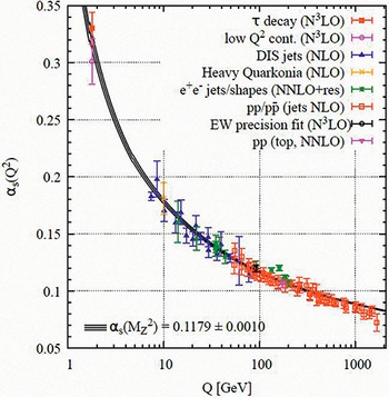
Figure 8.1 displays a plot of the observed running of the strong coupling
 as a function of probed energy for a wide range of processes and energy scales and its comparison to the QCD prediction. The agreement with the experiment results is well established and the running of the QCD coupling is quite apparent.

Figure 8.1 Summary of measurements [Reference Zyla, Barnett and Beringer62] of the running
 as a function of the energy scale
 . The agreement between the data and the QCD expectations is apparent. The order of QCD perturbation theory used in the extraction of
 is indicated in brackets (NLO: next-to-leading order; NNLO: next-to-next-to-leading order; NNLO+res.: NNLO matched to a re-summed calculation; N
 LO: next-to-NNLO).
The ramifications of asymptotic freedom were immediate and far reaching.Starting in 1968, SLAC began a series of experiments on the inelastic scattering of an electron from a proton:
 , where
 can be anything. Here
 are the 4-momentum of the incident (final) electron and
 is the 4-momentum of the incident proton. Using general properties of Lorentz covariance and electric charge conservation, the differential cross for this inelastic process due to a single photon exchange in the rest frame of the incident proton where
 ,
,
 and
and
 is the scattering angle between the initial and final state electrons takes the form
 (8.8)
(8.8)
Here
 is the momentum transfer,
 and
and
 . The
. The
 are the structure functions. In the rest frame,
 gives the electron energy loss.
It was observed [Reference Bloom, Coward and DeStaebler63; Reference Breidenbach, Friedman and Kendall64] (for a review, see [Reference Friedman and Kendall65]) that in the deep inelastic limit (sometimes referred to as the Bjorken limit) where
 at fixed
 , the structure functions were independent of
 and dependent only on the dimensionless scaling variable
 so
so
 . This behavior was previously suggested by Bjorken [Reference Bjorken66] and is consistent with scattering off point-like constituents of the proton. Similar scaling behavior was also observed in deep inelastic muon- and neutrino-scattering experiments conducted at FNAL.
This scaling behavior could be accounted for by the parton model introduced by Feynman [Reference Feynman67],[Reference Feynman68] in his study of hadron–hadron collisions. The “naive” parton model describes the proton as a collection of point-like constituents called partons. At high momentum (“infinite momentum frame”) the partons are taken as free. Therefore, the interaction of one parton with the electron does not affect the other partons and this leads to scaling in
 . Today these partons are understood to be identical with the quarks postulated by Gell-Mann [Reference Gell-Mann69] in 1964 and independently by G. Zweig [Reference Zweig70]. The quark-parton model was successfully applied by Bjorken and Paschos [Reference Bjorken and Paschos71] to reproduce the observed scaling in deep inelastic electron-proton scattering. The observation of Bjorken scaling in deep inelastic scattering was instrumental in providing the first dynamical evidence of quarks and then gaining their acceptance as constituents of the proton. While the quark-parton model produced the scaling behavior observed at the time, the model itself lacked a firm theoretical foundation. It was not a quantum field theory and could not account for the strong interquark forces needed to account for the nonobservation of the partons in remnants of the collision. Due to its asympototic freedom, QCD interaction strength falls at large momentum transfers as
 and thus behaves in a manner similar to the parton model. In fact, in subsequent experiments, deviations from the exact scaling behavior of the structure functions appeared. The scaling violations were precisely detected in a muon scattering experiment at FNAL in 1975 [Reference Chang, Chen and Fox72]. The observed
 dependence of the structure functions was accurately accounted for by QCD as reviewed in [Reference Ellis73], marking a major success of the theory.
In a grander sense, the concept of asymptotic freedom provided a sensible interpretation of a quantum field theory at extreme ultraviolet energies. For nonasymptotically free theories, the running coupling increases with increasing energy diverging at the Landau poleFootnote 2 [Reference Landau, Abrikosov and Khalatnikov74]. Asymptotic freedom in QCD also played an important role in theoretical work in early Universe cosmology. In the first few microseconds after the big bang, the Universe was comprised of a hot soup of quarks, leptons, gauge bosons and Higgs particles, which, as a consequence of asymptotic freedom, interacted very feebly and thus had properties amenable to calculation. This success in applying particle physics ideas to addressing puzzles in cosmology has led to a deep connection between the two disciplines, sometimes referred to as astroparticle physics, and has had a far-ranging influence on how one thinks about and treats cosmological problems. See [Reference Kolb and Turner75] for a readable introduction. Asymptotic freedom has also been displayed in a variety of condensed matter systems. For a discussion of various such systems, see, for example, reference [Reference Majorana151].
Motivated by the property of asymptotic freedom, it is suggestive that the attractive coupling grows at longer distances, leading to the confinement of all colored objects. Thus the quarks and gluons can never appear as physical states in the spectrum. Only net colored singlet hadrons (and glueballs) are physical states. Through the confinement mechanism, the potential long-range force that would naively arise from the massless gluons is obviated. This nonperturbative confinement mechanism has been demonstrated in lattice QCD [Reference Wilson77], which is a well-established nonperturbative approach to solving QCD. The lattice gauge theory is formulated on a grid or lattice of points in space and time. When the size of the lattice is taken infinitely large and its sites infinitesimally close to each other, the continuum QCD is recovered. Additional details can be found in [Reference Gattringer and Lang78–Reference Montvay and Münster80]. Lattice QCD has been used to compute the masses of the various hadrons as explicitly shown in reference [Reference Kronfeld81].
In the limit of massless up and down quarks, QCD exhibits the continuous global
 chiral symmetry, which is dynamically broken to
 via the formation of a nonvanishing quark-antiquark vacuum condensate, which in turn gives mass to the nucleons. The pions are the pseudo Nambu–Goldstone bosons of the spontaneously broken axial
 . (The pions develop a small mass as a consequence of the up and down quark mass, which provides a small explicit breaking of the
 symmetry). Thus QCD automatically displays the global symmetry structure of the strong interactions.
QCD has been very well tested and proven highly successful [Reference Zyla, Barnett and Beringer62]. It constitutes one of the components of the Standard Model.
9
Invariant Lepton Couplings to the Electroweak Vectors

As we have seen, simply adding a vector mass term to the Lagrangian violates the gauge invariance. However, in 1962, J. Schwinger argued that the gauge invariance might not preclude a vector mass once the radiative corrections are included, provided the current coupling to the vector is sufficiently strong that it can create a massless pole in the current-current correlation function,
 . In that case, the full vector propagator varies as
 (9.1)
(9.1)
which corresponds to a massive particle. The nonzero mass is said to be dynamically generated. While he was unable to demonstrate the existence of such a pole in any Lorentz-invariant model containing vectors in four space-time dimensions, he showed it was possible in a two space-time dimensional model, the Schwinger Model. In a very short, but extremely elegant paper [Reference Schwinger82], he studied a version of QED but in one space and one time dimension and with massless fermions. Since the fermions were massless, the QED
 Lagrangian exhibits separate phase invariances for vector and axial vector transformations. Schwinger analytically solved the model and found a dynamically generated fermion-antifermion condensate that spontaneously breaks the axial symmetry and moreover the vacuum polarization function does indeed develop a massless pole so that the “photon” gets a nonvanishing mass. Although one can legitimately argue that the mass-generating mechanism is an artifact of the 1+1-dimensional nature of the model, this paper nonetheless was (and continues to be) extremely influential in that it showed that “vector” masses were possible in gauge theories.
A further elucidation of this idea was provided by P. Anderson [Reference Anderson83] in 1963 who argued that the gauging of the spontaneously broken global continuous
 symmetry in BCS theory essentially leads to a massive vector photon, which was then unable to penetrate the superconductor (Meissner effect [Reference Meissner and Ochsenfeld84]). Here the massless pole is provided by the massless phonons mediating between the Cooper pairs in the superconductor. The model provided a mechanism for vector mass generation in a nonrelativistic setting. Much discussion in the literature followed regarding the general applicability of Anderson’s ideas to relativistic theories without any definitive resolution at the time.
Actually, there is an even earlier realization of the vector mass generation mechanism. In 1938, E. Stueckelberg [Reference Stueckelberg85] proposed a model of massive quantum electrodynamics using an additional scalar field that nonlinearly realized the symmetry. Like much of his work, it was well ahead of its time and largely ignored.
While the simple mimicking of QED by introducing vector bosons with direct mass terms was not an accurate description of the weak interactions, there was still considerable motivation for believing that the correct description should involve vector and axial vector fields. For one thing, the parity-violating extension of the Fermi theory was quite successful in describing low-energy, weak-interaction processes using lowest-order perturbation theory. A nice description of the phenomenological theory of the weak interactions before the advent of the electroweak gauge theory is contained in the monograph [Reference Källén86]. In addition, the Fermi description involved currents as did QED, albeit electric-charge-carrying currents that were both of a vector and an axial vector nature and moreover the hadronic piece of the vector current was conserved as is the vector current in QED. Finally, another property of the weak interactions where the resemblance to QED is striking is its universality [Reference Pontecorvo87],[Reference Puppi88]. That is, the weak processes of
 decay, muon decay and muon capture all had basically the same strength. This is reminiscent of the common magnitude of the electromagnetic charge of electrons, muons and protons.
J. Schwinger [Reference Schwinger40] was the first who attempted (unsuccessfully) to combine weak and electromagnetic interactions together in an
 Yang–Mills gauge theory using the charged massive
 and massless photons as the gauge vectors. His student S. Glashow [Reference Glashow89] and independently A. Salam and J. Ward [Reference Salam and Ward90] did arrive at a model of leptons based on the gauge group
 , which includes the correct couplings of the leptons to the electroweak gauge bosons. The model has two independent coupling constants
 associated with the
 and
and
 gauge groups respectively. The product group has four generators and four associated vector bosons. To reproduce the V-A structure of charged weak interaction, the left-handed electron and its associated neutrino transform as a doublet,
 , under
 , while the right-handed electron,
 , is an
 singlet. Here we focus on the first generation of leptons consisting of the electron and its associated neutrino. The inclusion of the other lepton families is straightforward and will be discussed shortly. The model includes no right-handed neutrino field. To secure the couplings to the vector bosons, one follows the usual procedure of replacing
 and
and
 in the leptonic kinetic terms. Here the covariant derivatives are
 (9.2)
(9.2)
where
 ;
;
 are the three Pauli matrices. The resultant locally invariant
 Lagrangian is
 (9.3)
(9.3)
The electron and its associated neutrino couplings to the gauge fields are thus dictated by the local
 invariance to be
 (9.4)
(9.4)
where the
 and
and
 electron family currents are
 (9.5)
(9.5)
 (9.6)
(9.6)
Two of the conserved currents of
 ,
,
 (9.7)
(9.7)
are identified with the weak-interaction charged currents, which couple to the associated vectors
 (9.8)
(9.8)
as
 (9.9)
(9.9)
There are two neutral generators: the third component
 of the weak isospin
 and the weak hypercharge generator
 of the
 . One combination is identified as the electric charge generator
 (9.10)
thus fixing the weak hypercharges with their values appearing in the covariant derivatives so that the electron has electric charge
 1 and the neutrino is neutral.
The photon is identified as
 (9.11)
which is the combination of vector bosons which couples to the electromagnetic current
 (9.12)
as
 (9.13)
Here
 , the Weinberg angle, is a weak mixing angle (the angle
 was originally introduced by Glashow as the weak mixing angle but has subsequently been universally referred to as the Weinberg angle), satisfying
 (9.14)
In addition, the model predicted a novel weak neutral current
 (9.15)
which couples to a novel vector boson
 (9.16)
as
 (9.17)
The muon and its associated neutrino and the tau and its neutrino have identical
 quantum numbers as the electron and its neutrino (see Table 9.1). Thus their invariant couplings to the electroweak gauge bosons have the same structure as the electron and its neutrino and the model exhibits a lepton universality. The full lepton-gauge interaction is then a sum of the three generations of leptons:
Table 9.1 Weak isospin and weak hypercharge of the leptons.
| Lepton |

|

|
|---|---|---|

| 2 |

|

| 1 |

|
 (9.18)
The model introduced by Glashow, Salam and Ward is very incomplete:
There is no consistent mechanism for generating the
and
vector masses.All leptons are massless, which is experimentally inaccurate.
The model does not include quarks. The reason was that at the time the only known quark flavors were
,
, and
and the model extended to include them predicted far too large a rate for flavor (strangeness) changing neutral current (FCNC) processes such as
.


The model was successfully extended to include quarks in 1970 after the implementation of the S. Glashow, J. Iliopoulos, L. Maiani (GIM) mechanism [Reference Glashow, Iliopoulos and Maiani91], which introduced the
 quark with the appropriate Cabibbo angle [Reference Cabibbo93] mixing to provide a cancellation mechanism suppressing the dangerous FCNC processes. The
 quark was subsequently discovered independently at the Brookhaven National Laboratory [Reference Aubert, Becker and Biggs94] and at SLAC [Reference Augustin, Boyarski and Breidenbach95] through the observation of the J/
 meson. This mechanism was later extended by M. Kobayashi and T. Maskawa [Reference Kobayashi and Maskawa96] to allow for the inclusion of the third-generation
 and
and
 quarks, which could further account for the observed CP-symmetry violation [Reference Christenson, Cronin, Fitch and Turlay92] in the electroweak interactions. The left-handed quark fields transform as doublets under
 while the right-handed quark fields are
 singlets. The weak hypercharge assignments lead to the electric charges
 ,
,
 as shown in Table 9.2.
Table 9.2 Weak isospin and weak hypercharge of quarks.
| Quark |

|

|
|---|---|---|

| 2 | 1/6 |

| 1 | 2/3 |

| 1 |
 1/3
1/3 |
Identical quantum numbers are assigned to the other generations of quarks by simply replacing
 with
with
 and
and
 .
.
10 Abelian Higgs Model
It was clear that the symmetry of the electroweak model had to be realized à la Nambu–Goldstone. What remained a major stumbling block was how to circumvent the theorem which mandated the presence of unobserved massless Nambu–Goldstone bosons. The solution was inadvertently arrived at in 1964 by R. Brout and F. Englert [Reference Brout and Englert97] and independently by P. Higgs [Reference Higgs98]. Slightly later, G. Guralnik, C. R. Hagen and T. Kibble [Reference Guralnik, Hagen and Kibble99] also discussed in more detail how the massless NGB mode could be obviated. Another independent version of the mechanism was provided by A. Migdal and A. Polyakov [Reference Migdal and Polyakov100]. (Although the time line of this publication is significantly behind the other work, it has been said that this was due to an initial rejection by the journal JETP to which it was submitted. No date has ever been substantiated for the original submission.)
The basic idea is to gauge the spontaneously broken global symmetry. The mechanism was actually initially presented in a simplified
 toy model. Recall the global
 symmetry of the Goldstone model and now promote it to a local Abelian U(1) symmetry, which yields the so-called Abelian Higgs Model. The model Lagrangian

with
 (10.1)
 (10.2)
and
 (10.3)
is invariant under the local U(1) transformations
 (10.4)
If
 , the potential has the sombrero form displayed previously and is minimized for
 with
with
 . Once again parametrizing
 (10.5)
with Hermitian
 , the model Lagrangian (neglecting any field-independent terms) takes the form
 (10.6)
with the ellipses denoting cubic and quartic interaction terms. Performing the gauge transformation

the second term is recognized as a mass term for the vector
 with mass
 . The scalar
 is also massive, with
 . On the other hand, there is no kinetic term nor mass terms for
 , so its dynamics appears to have vanished. The apparently massless vector gauge field
 and the apparently massless scalar field
 (the erstwhile Nambu–Goldstone mode) have combined to produce the massive vector field
 . The Nambu–Goldstone mode has become the longitudinal degree of freedom needed to provide the vector its mass. The number of degrees of freedom has not changed. In the vernacular, one says the NGB is eaten by the massless vector giving it mass. This is the celebrated Higgs mechanism. (Although it might be more properly called the Stuekelberg–Schwinger–Anderson–Brout–Englert–Higgs–Guralnik–Hagen–Kibble–Migdal–Polyakov–Weinberg–Salam–
 mechanism.)
For every spontaneously broken global symmetry which is made locally (gauge) invariant, the erstwhile NGB is absorbed by the vector to become its longitudinal component, rendering the vector massive. This is true independent of the dynamics responsible for spontaneously breaking the global symmetry. The massive scalar mode (which in this toy model is the analog of the physical Higgs scalar) remains. The mechanism was extended by Brout, Englert and Higgs to non-Abelian models. Brout and Englert also mentioned the possibility of having a composite fermion-antifermion condensate be responsible for the symmetry breakdown. In all the papers, the motivation for the vector mass generation mechanism was that it be used in the strong interactions. None of the original authors foresaw its application to the weak interactions. Brout and Englert do not even mention the massive scalar mode in their 1964 paper. Higgs submitted two papers in 1964. The second paper was initially rejected, and the revised version does indeed mention the possible experimental implication of such a massive scalar in the spectrum. Guralnik, Hagen and Kibble also fail to discuss the massive scalar in their 1964 paper. So how is it possible to avoid the physical massless scalar degree of freedom when the spontaneously broken symmetry is gauged?
As alluded to previously, Goldstone, Salam and Weinberg [Reference Goldstone, Salam and Weinberg47] provided a proof of a theorem that mandates the emergence of a NGB mode in any theory each time the following three conditions are met:
(i) The appearance of a continuous global internal symmetry and corresponding conserved Noether current.
(ii) Said symmetry is spontaneously broken so there is a degenerate family of vacuum states and there exists a field (possibly composite) which carries a nontrivial charge of the spontaneously broken symmetry and whose vacuum expectation value is nontrivial.
(iii) The theory is manifestly Lorentz invariant.
Note that this last requirement is needed to guarantee the appearance of the Nambu–Goldstone bosons. While NGBs may also appear in theories with spontaneously broken global space-time symmetries or spontaneously broken global internal symmetries in Galilean invariant theories, they are not mandated to do so in all such cases while they are for manifestly Lorentz-invariant theories.
What fails in the case of gauge theories? To quantize a gauge theory, one must choose a gauge and impose a gauge-fixing condition. For the
 gauge theory, a massless vector field has four components, but only two of them are physical (the transverse modes). One type of gauge choice, the Coulomb gauge defined by
 and
and
 , explicitly eliminates the unphysical degrees of freedom. But the price one pays for this is the loss of manifest Lorentz invariance and an evasion of the theorem ensues. Alternatively, one could choose a manifestly Lorentz-covariant, gauge-fixing term such as a Landau gauge
 . In this case, the Hilbert space necessarily contains the unphysical longitudinal and scalar degrees of freedom. Here the theorem does apply, but the contribution of the Nambu–Goldstone degrees of freedom to any physical process precisely cancels against the unphysical photon modes, so effectively these modes are uncoupled from the physical particles in the theory. Note that even though one must fix a gauge to quantize the model, the theory is very clever and all physical quantities are gauge and Lorentz invariant.
11 Standard Electroweak Model
In 1967, S. Weinberg [Reference Weinberg101] and A. Salam [Reference Salam and Svartholm102] independently developed a model of the electroweak interactions of leptons based on the gauge group
 using the Glashow and Salam–Ward model quantum number assignments and current identifications, but now exploiting the Higgs mechanism to give mass to the charged and neutral weak vector bosons while keeping the photon massless. Moreover, they exploited the Schwinger mechanism to generate the charged lepton masses. Explicitly, they introduced an
 doublet of scalar fields (four degrees of freedom), which also carries weak hypercharge (
 1/2). The scalars had a self-interacting potential function of the Brout–Englert, Higgs, Goldstone, Ginzburg–Landau form
 (11.1)
A nonzero vacuum expectation value,
 , is generated for the neutral component of the scalar doublet spontaneously breaking the
 symmetry while leaving a residual unbroken electromagnetic symmetry
 so that
 . These scalars were coupled to the gauge fields via the covariant derivatives. The gauge vector of this unbroken symmetry was identified with the massless photon. The three erstwhile NGBs of the spontaneously broken symmetries became, via the Higgs et al. mechanism, the longitudinal components of the
 and
and
 vectors endowing them with masses, which satisfies
 (11.2)
(For details, the reader is directed to Appendix A.2.) Note that this relation follows as a consequence of using a scalar
 doublet to spontaneously break the symmetry. Let us focus on the preceding Higgs potential. Said potential actually exhibits a global
 symmetry, which contains the global
 as a subgroup with the third generator of the
 identified with the weak hypercharge generator
 . This larger symmetry of the Higgs potential is not respected by the full electroweak Lagrangian, as it is explicitly broken by the gauging of the hypercharge and the differing Yukawa couplings between the upper and lower components of the
 fermion doublets so that the full Lagrangian has the
 symmetry. When the scalar doublet acquires its nontrivial VEV, the global
 symmetry of the Higgs potential is spontaneously broken to a residual global
 symmetry. This residual
 symmetry is the diagonal subgroup of the
 and is referred to as a custodial symmetry [Reference Sikivie, Susskind, Voloshin and Zakharov103]. Note the unbroken electric charge generator,
 , is the third component of the custodial
 . If the spontaneous symmetry breaking is engendered by scalar fields transforming other than as doublets acquiring nontrivial VEV, the resulting Higgs potential will not exhibit the custodial
 symmetry and Eq. (11.2) will have no longer be satisfied.
The electroweak model has two independent gauge couplings whose values are extracted from experiment. The particular experiments employed to do so are often chosen to be those which are very accurately measured. One such choice is the electromagnetic fine structure constant. Two independent methods have been used. One uses the electron anomalous magnetic moment [Reference Zyla, Barnett and Beringer62] to give
 , while an independent determination [Reference Morel, Yao, Cladé and Guellati-Khélifa17] employs atomic interferometry in rubidium atoms to yield
 . Note that using the latter measure allows for a comparison between theory and experiment in the
 determination. The second coupling is fixed by the Fermi constant, which is best secured today by comparing the calculation of the muon lifetime with the experimentally measured result [Reference Zyla, Barnett and Beringer62] giving
 . Thus while the theory is such that weak and electromagnetic interactions have a common origin, it is not technically a unified theory, which would have only a single coupling. The nontrivial VEV is then fixed by the Fermi scale as
 (11.3)
Very little attention was paid to the Glashow–Salam–Weinberg (GSW) model when it was first introduced. The turning point came in 1971, when G. ‘t Hooft [Reference ’t Hooft104] (see also [Reference Veltman105–Reference Lee109]) proved that the model was renormalizable and hence consistent order by order in perturbation theory. The key was that the vector mass generation mechanism arose in a non-Abelian gauge theory using the Higgs mechanism. Since it is a Yang–Mills gauge theory, the vector propagator can be taken to have the same type of large momentum falloff as the photon propagator in QED even though the electroweak gauge bosons are massive.
A major breakthrough in the experimental verification of the model came with the discovery of the neutral current interactions in neutrino experiments using the Gargamelle bubble chamber at CERN in 1974 [Reference Gargamelle Collaboration, Faissner and Krenz110; Reference Gargamelle Collaboration, Kabe and Krenz111]. The results of this experiment were consistent with the structure of the neutral current interactions as detailed in the GSW model.
In fact, long before the neutral current was observed, it was conjectured that they could exist and have parity-violating effects that could be detected [Reference Zel’dovich and Exp112] in both electron scattering experiments and via atomic spectra measurements. More than 20 years after this proposal, parity violation in the weak neutral current was indeed measured in polarized electron-deuteron scattering at SLAC [Reference Prescott, Atwood and Cottrell113; Reference Prescott, Atwood and Cottrell114]. The agreement of this experiment with the predictions of the GSW model firmly established it as the leading candidate to describe electroweak interactions. The dominant contribution to the atomic bound state energy levels arises from the parity-conserving electromagnetic interaction between the electrons and the protons mediated by photon exchange. In addition, there will also be a contribution from the weak neutral current arising from the
 boson exchange. Since the neutral current interactions in the GSW model contain a parity-violating component, the interference term of these two contributions results in the various levels receiving a small admixture of the opposite parity. While an accurate quantitative estimate (for a general review see, for example, [Reference Khriplovich115]) of this admixture requires detailed atomic physics calculations, for atomic number
 , the effect is roughly of order
 . The
. The
 enhancement factor for large
 was first pointed out in [Reference Bouchiat and Bouchiat116]. Additional enhancement mechanisms can be employed to make the effect in cesium as large as
 . The first such parity-violating signal was observed in 1978 by L. Barkov and M. Zolotorev [Reference Barkov and Zolotorev117] in Bi atoms. Over the following decades, parity violation has been observed in a variety of atoms, with the most accurate measurements made in Cs [Reference Wood, Bennett and Cho118] by the Wieman group at Boulder.
In 1983, the
 and
and
 vector bosons were discovered by the UA1 and UA2 collaborations at CERN [Reference Arnison, Aniston and Aubert119–Reference Bagnaia, Banner and Battiston122]. The world average of the measured masses is currently [Reference Zyla, Barnett and Beringer62]
 (11.4)
Using these measured masses, the weak mixing angle defined as
 is determined as
 .In Appendix A.2, the full
 electroweak model Lagrangian is presented in detail.
Tables 11.1 and 11.2 are taken from the particle data book [Reference Zyla, Barnett and Beringer62] and provide a global fit to a variety of electroweak processes and the comparison to the Standard Model expectation. The agreement with the SM expectation is very good and the global electroweak fit describes the data very well. As of today, the electroweak model has been very precisely tested experimentally in a huge variety of different experiments covering a range of energy scales from the atomic level (eV) to the scale of the LHC (TeV) and its success constitutes a remarkable achievement.
Table 11.1 Standard Model prediction compared with experimental results secured using the LEP detector at CERN, which precisely measured various parameters in the
collisions with total incident energy tuned to be near the
mass.
is total cross section to hadrons and
is the total
decay width.
;
for
and
where
is the partial width for
decays to hadrons and
are the partial widths for
with
;
is the forward-backward asymmetry for fermion
;
is the left-right asymmetry for fermion
. Note that the three values for
are consistent with lepton universality. The column denoted by Pull gives the standard deviation from the SM prediction.


| Quantity | Experiment | Standard Model | Pull |
|---|---|---|---|
 [GeV]
[GeV] |

|

|

|
 [GeV]
[GeV] |

|

| 0.6 |
 [nb]
[nb] |

|

| 0.0 |

|

|

| 1.4 |

|

|

| 1.4 |

|

|

|

|

|

|

| 0.7 |

|

|

| 0.0 |
 (e)
(e) |

|

|

|
 (b)
(b) |

|

|

|
 (c)
(c) |

|

|

|
 (s)
(s) |

|

|

|

|

|

| 2.1 |

|

| 0.9347 |

|

|

| 0.6677
 0.0001
 | 0.1 |

|

| 0.9356 |

|
Table 11.2 Standard Model prediction compared with experimental results for non-
pole observables.
is the top quark mass,
is the Higgs boson mass,
is the
mass and
is the
width;
are the leptonic vector and leptonic axial vector couplings and
is the lepton lifetime,
. The weak charges
(Cs) and
(Tl) are extracted from atomic physics parity violation experiments in Cs and Tl. The column denoted by Pull gives the standard deviation from the SM prediction.


| Quantity | Experiment | Standard Model | Pull |
|---|---|---|---|
 [GeV]
[GeV] |

|

| 0.5 |
 [GeV]
[GeV] |

|

| 0.0 |
 [GeV]
[GeV] |

|

| 1.6 |
 [GeV]
[GeV] |

|

|

|

|

|

| 0.0 |

|

|

| 0.0 |
 (Cs)
(Cs) |

|

| 1.0 |
 (Tl)
(Tl) |

|

| 0.1 |
 [fs]
[fs] |

|

| 0.8 |
One present potential outlier is the measurement of the anomalous magnetic moment of the muon
 . The muon anomalous magnetic moment is a particularly promising quantity to investigate since any beyond-the-Standard-Model contribution scales like
 , where
 is the mass scale of the beyond-the-Standard-Model physics. Hence, the sensitivity of
 is enhanced relative to
 by a factor
 . Moreover,
 has been measured with a precision of 0.46 ppm [Reference Abi, Albahri and Al-Kilani124], which is much more precise than what can currently be achieved experimentally for
 , which would, in principle, be an even more sensitive measure.
The SM expectation
 has been reported in a 2020 White Paper [Reference Aoyama, Asmussen and Benayoun123] by the Muon
 Theory Initiative. The quoted overall precision of 0.37 ppm is limited by contributions due to the strong interaction, notably the contributions from hadronic vacuum polarization and to a lesser extent by the hadronic contribution to light-by-light scattering. This recommended value for
 is based on the “data-driven” evaluation of the hadronic vacuum polarization contribution, which is determined using dispersion relations and the experimentally measured hadronic cross sections in
 collisions. Combining the run 1 data of the Fermilab Muon g-2 experiment [Reference Abi, Albahri and Al-Kilani124–Reference Albahri, Anastasi and Badgley126] reported in 2021 and the previous measurement at the Brookhaven National Laboratory E821 Collaboration [Reference Bennett, Bousquet and Brown127] results in a world average of
 , which differs from the previously mentioned SM prediction of
 by
by
 , which constitutes a 4.2
 discrepancy. If this result persists, it indicates a violation of electron-muon universality beyond just the differences in their masses.
Lattice QCD provides an alternative theoretical calculational scheme to the data-driven methodology. Using an average of the lattice results available at the time, the Muon
 -2 Theory Initiative White Paper [Reference Aoyama, Asmussen and Benayoun123] reported a higher value of
 than that found using the data-driven method, but still consistent within the uncertainties. Subsequently, a lattice QCD result [Reference Sz. Borsanyi and Guenther128] for the hadronic vacuum polarization was published that reduced the difference between the SM and the experimental result to
 . They also estimated a
 tension in the hadronic contribution to the running of
 than that determined using the
 data. Clearly, an independent cross-check of the [Reference Sz. Borsanyi and Guenther128] lattice result is sorely needed.
Occasionally, other hints of deviations from the model have arisen. But thus far, none have stood the test of time.
A very nice demonstration of how the various elements of the Standard Model are required in order to have agreement with experiment is provided by the LEP measurement at CERN of the
 cross section. At leading (second) order in perturbation theory, various Feynman graphs contribute: neutrino exchange, photon exchange and
 exchange, as shown in Figure 11.1. (There is also a Higgs exchange graph, which gives a contribution of
 relative to the other graphs and can be safely ignored.) The neutrino exchange graph arises from the charged current interaction, while the photon exchange and
 exchanges mediate the electromagnetic and neutral current interactions respectively. Note that the
 exchange graph involves the triple gauge vector
 vertex, which is mandated by the non-Abelian gauge structure. Plotted in Figure 11.2 is the LEP measurement as well as the predicted cross section with only neutrino exchange, no
 vertex and with all three as required by the Standard Model. Clearly all three interactions are required for agreement.

Figure 11.1 Leading-order Feynman graphs contributing to
 .
.

Figure 11.2 Measurements from LEP of the production cross-section
 compared to the SM calculation of the RACOONWW [Reference Denner, Dittmaier, Roth and Wackeroth130], YFS [Reference Jadach, Placzek, Skrzypek, Ward and Was131] and GENTLE [Reference Bardin, Biebel and Lehner132] collaborations. The plot is secured from the ALEPH, DELPHI, L3, OPAL and LEP Electroweak Collaborations [129].
In the SM, the
 vector boson couples directly via the neutral current interaction to
 where
where
 is any fermion and to
 . It also couples to
 with
with
 the Higgs boson. Note there is no direct coupling of the
 to a pair of photons. Using the LEP detector at CERN, the
 beam energy was tuned to scan the region in the vicinity of the
 mass. In that case, the
 and
and
 final states do not contribute since the
 and
and
 have masses well in excess of
 . Thus the only final states that contribute are
 , where
 can be any of the three charged leptons, any quark (which will fragment into hadrons) other than the
 quark and any possible neutrino whose mass is less than
 .
.
The annihilation cross section [133] for
 is generally fit to the Breit–Wigner form
 (11.5)
which accounts for a process in which a spin one particle is produced in
 collisions and then annihilates into an
 channel in the resonance region for the case where the resonance width is much less than the vector mass. This typical resonance shape peaks around the
 mass,
mass,
 , and has a total width
 . If the
 decays a fraction
 of the time into a final state
 , the corresponding partial width is defined as
 . For the moment, we assume that there are
 neutrino species that contribute. In that case, the total
 width is simply
 (11.6)
The LEP detector separately measured the total width
 from the shape of the resonance curve as well as the hadronic width,
 (
(
 ) and each charged leptonic width
 (
(
 ). Using the Standard Model calculation of
 , the only unknown is
 , the number of light neutrino species. Figure 11.3 displays the line shape for
 . The fit to the data yields
 , which is in excellent agreement with the observed number of fermion generations:
 .
.

Figure 11.3 The
 annihilation cross section as a function of center-of-mass energy in the vicinity of the
 pole, as measured by the LEP experiments [133]. The curves represent the Standard Model predictions for two, three and four species of light neutrinos. It is clear from this picture that there is no further light neutrino species with couplings identical to the first three.
12 The Higgs Boson
By 2012, the only as yet undetected ingredient of the Standard Model was the Higgs scalar
 . As detailed in Appendix A.2, it couples to all massive bosonic particles in proportion to the square of the boson mass and to fermionic particles linearly in the fermion mass. Furthermore, the generalized Yukawa couplings to the fermions also allow for the observed flavor-changing charged weak interactions parametrized by the Cabibbo–Kobayashi–Maskawa (CKM) matrix [Reference Cabibbo93; Reference Kobayashi and Maskawa96]. (For the experimentally determined CKM parameters, see [Reference Zyla, Barnett and Beringer62].) The Higgs scalar is self-coupled and massive
 . The model, however, does not fix the value of this mass, which must be determined experimentally. This was achieved in 2012 when the CMS and Atlas collaborations at the CERN LHC announced the discovery [Reference Aad, Abajyan and Abbott1; Reference Chatrchyan, Khachatryan and Sirunyan2] of a scalar particle with mass
 125 GeV whose properties were consistent with that of the Standard Model Higgs boson.
The dominant decay channel of a Higgs scalar with such a mass is into
 with a branching fraction [Reference Zyla, Barnett and Beringer62]:
 . However, at hadron colliders such as the LHC, this mode is masked by the presence of very large backgrounds, making the identification of a Higgs boson signal in these channels quite challenging. Hence the CMS and Atlas collaborations focused on the decay of the Higgs scalar into two photons:
 . Since the photon is massless, there is no direct coupling to the Higgs field. The leading contribution to this process comes from the 1-loop diagrams, with the more massive charged particles traversing the loop giving the dominant contributions. This corresponds to the top quark and the
 boson as shown in Figure 12.1.

Figure 12.1 Examples of Feynman graphs contributing to
 . In the first diagram,
 can be any charged, massive fermion with the dominant contribution coming from the top quark traversing the loop.
Consequently, the branching fraction [Reference Zyla, Barnett and Beringer62] for this mode is small:
 . Nonetheless, an unambiguous signal was successfully detected. Subsequently, additional decay channels including
 have been observed and analyzed. In all cases, consistency with the properties of the Standard Model Higgs boson persists. As of this writing, the mass of this scalar is measured [Reference Zyla, Barnett and Beringer62] as
 (12.1)
A few comments are in order.
One really needs to distinguish between the existence of the Higgs et al. mechanism and the particular way it is engendered. The Higgs mechanism that gives mass to the weak interaction vector bosons results whenever a spontaneously broken global continuous symmetry is made locally invariant independent of the dynamics responsible for the spontaneous symmetry breakdown. It was actually validated in 1983 with the discovery of the massive
and
vector bosons. With the discovery of a light Higgs scalar particle, it appears this mechanism arises in the electroweak model through the interactions of a perturbatively coupled scalar field sector based on the type proposed by Brout–Englert and Higgs and others. The physical dynamics implementing the vector mass generation mechanism did not necessarily have to be of this form. For example, it could have been some new interaction leading to a fermion-antifermion condensate breaking the electroweak symmetry more in analogy to what happens in BCS or to the chiral symmetry breaking in QCD. In that case, the “Higgs scalar” would not be nearly as light as it turned out.The Higgs mechanism as implemented in the Standard Electroweak Model is extremely economical. With the addition of one novel scalar physical degree of freedom, one generates nonzero masses for the weak gauge vectors and the fermions as well as incorporates the observed Cabibbo–Kobayashi–Maskawa quark flavor mixings and CP-symmetry violation in a mathematically consistent framework. Nature apparently has chosen the highly economical and simplest, albeit arguably not the most satisfying route. While all the rest of the dynamics in the Standard Model is determined via interactions with the gauge bosons, the scalar self-couplings responsible for the symmetry breaking and the Yukawa couplings to the scalar fields are not.
Contrary to what sometimes appears in the literature, the Higgs mechanism is not responsible for most of the visible (i.e. nondark matter) mass in the Universe. The predominance of visible mass is protons and neutrons. Most of their mass results from the QCD binding of their quark and gluon constituents. Up and down quark masses do arise from the Higgs mechanism, but their contribution to the proton mass is very small (a few parts in a thousand). However, the fermion masses generated via the Higgs/Schwinger mechanism are crucial. Without it, QCD still confines quarks into protons so the nucleon mass would be basically unchanged. However, now the electroweak symmetry would be broken by the formation of QCD vacuum chiral condensates at a much lower scale (
250 MeV). The W and Z bosons would acquire mass of this order by absorbing the Nambu–Goldstone boson pions. Because the electron would be massless in the absence of the Higgs/Schwinger mechanism, the atomic Bohr radius would be infinite. There would be nothing recognizable as an atom, no chemistry as we know it, no stable composite structures like solids or liquids. None of us would exist!


13 Global Symmetries versus Local Invariance
We have traced the development of the Standard Model of particle physics by following how its various symmetries were uncovered and implemented. While recognizing that global symmetries played a crucial role in this story, as it turns out, the global symmetry structure is actually an automatic consequence of the local invariance. That is, once the gauge group and transformation properties of the matter fields under said group are specified, the dynamics is determined and so is the global symmetry structure, which does not have be separately mandated and enforced.
The case of gauge invariance is somewhat more subtle. Calling an invariance under local transformations a symmetry (gauge symmetry) is actually a misnomer. When one speaks of a symmetry in a quantum theory, what one really means is the invariance under transformations of the quantum states that lie in a Hilbert space. However, a gauge transformation does not change the quantum states (it acts trivially on the Hilbert space) and hence it really should not be called a symmetry. Rather the gauge invariance dictates that the excitations of certain fields appearing in the action functional do not really produce physical states. Thus the gauge symmetry actually corresponds to a redundancy of the theoretical description, which is introduced to insure that the theory is local. This is why the gauge invariance of the underlying action functional must be exactFootnote 3 and cannot be broken by the inclusion of additional non–gauge-invariant local operators without destroying the consistency of theory. With the inclusion of such non–gauge-invariant terms in the action, the unphysical degrees of freedom would not be eliminated, leading to a violation of some basic principle such as Lorentz invariance or positivity of the state space norm, which corresponds to a breakdown of causality or unitarity (probabilities exceeding unity).
The same argument applies to the case where one attempts to gauge a symmetry of the Lagrangian which is broken by quantum radiative corrections arising from fermion loops. In such a case, the symmetry is said to be anomalous. Anomalies [Reference Adler134, Reference Bell and Jackiw135] reflect an intrinsic breaking, which cannot be compensated by adding local counterterms in higher orders of perturbation theory. Thus any potential anomalies associated with the dynamical gauge currents need to be canceled if the dynamical gauge invariance is to be preserved.
Since the anomalies depend only on the charge structure of the dynamical fermions traversing the loops, their cancellation constrains the fermion matter content of many gauge field theories. The nonrenormalization theorem [Reference Adler and Bardeen136] guarantees that this cancellation will be preserved to all orders. From the form of the non-Abelian anomaly [Reference Bardeen137], it can be shown that models with vectorlike gauge couplings, such as QED or QCD, do not have dynamical anomalies. Only theories where the fermions have chiral gauge couplings can have nontrivial anomalies. If the standard electroweak model is based on a chiral gauge theory, the individual fermions propagating in the loop produce anomalies, but are canceled between the various quark and lepton contributions.
This is contrary to the case of global symmetries where globally nonvariant local terms can be added to the action without destroying the consistency of the theory. The only way to “break" a gauge symmetry is by making the spontaneously broken global theory locally invariant. But this operation is not a deformation of the theory (as is the case of adding globally noninvariant terms to an otherwise globally invariant theory), but rather corresponds to a different theory altogether. There is also no restriction on having anomalous global symmetries. In fact, the existence of an anomaly in the axial vector global current is responsible for the experimentally observed decay mode of the neutral pion to two photons.
14 Limitations and Challenges of the Standard Model
Despite being the most successful theory of particle physics to date, the Standard Model is still neither complete nor totally satisfying. Here we briefly address shortcomings of the model.
 Standard Model parameters: Various parameters appear in the Standard Model. The form of the gauge groups and the quantum numbers of the fermions and scalars under said gauge groups are taken as given a priori. The same can be said of the 3+1 dimensionality of space-time. In addition, as in any quantum field theory, the Lagrangian must be supplemented by various normalization conditions before it is completely defined and used to make unambiguous predictions. The Standard Model depends on 19 parameters, each of which requires a normalization condition that can be fixed by experiment. These include the three gauge couplings, the three charged lepton masses, the six quark flavor masses, the three CKM mixing angles, one CKM phase and two parameters from the scalar sector that can be taken as the Higgs boson mass and the electroweak scale. In the Standard Model, only massless left-handed neutrinos appear.
A variety of beyond-the-Standard-Model proposals have been forwarded in an attempt to reduce the number of said parameters. Thus far, none have successfully achieved this goal. One approach posits the existence of a unified gauge group with a single gauge coupling that spontaneously breaks at a very high energy scale to the Standard Mode direct product gauge groups. While these Grand Unified Theories (GUTS) replace the three gauge couplings of the SM with one unified gauge coupling, all such models need to introduce a plethora of new particles and a large number of additional couplings both to achieve the unification and to engender the appropriate spontaneous symmetry breaking. Thus far, none of these have been observed. In addition, one experimental consequence of many GUTS is the finite lifetime of the proton and, as yet, all experimental searches have yielded null results. A review of GUTS is provided in [Reference Ross138].
In addition, there is another hitherto neglected parameter in the QCD Lagrangian,
 , which is the coefficient of the gauge-invariant Lagrangian term
 (14.1)
where
 is the gluon field strength and
 (14.2)
is the field strength dual. This gauge-invariant CP-symmetry-violating product is a total divergence [Reference Bardeen140],
 (14.3)
of the gauge-variant combination
 (14.4)
Being a total divergence,
 never contributes in any perturbative calculation. However, the QCD vacuum has a nontrivial structure, and nonperturbative effects can become important. Experimentally, the size of
 is constrained by measurements of the CP-symmetry-violating electron dipole moment (EDM) of the neutron. So far, no neutron EDM has been observed and the current experimental limit [Reference Abel, Afach and Ayres139] is
 e cm. The violation of CP-symmetry in the SM through the CKM phase gives
 e cm, which is far smaller than the error bars on the current bound. Since the
 parameter provides another possible source of CP-symmetry violation, the measurement of the EDM of the neutron restricts it to satisfy
 . The origin of the smallness of this dimensionless parameter is referred to as the strong CP problem. One possible solution is afforded by the Peccei–Quinn mechanism [Reference Peccei and Quinn141],[Reference Peccei and Quinn142], which introduces some additional degrees of freedom and an additional
 spontaneously broken anomalous symmetry, which allows this parameter to be effectively removed. There is a residual effect in the form of a novel pseudoscalar particle, the axion [Reference Weinberg143],[Reference Wilczek144], which is actively being hunted experimentally [Reference Zyla, Barnett and Beringer62]. The pseudo-NGB axion mass is model dependent but is roughly given by
 , where
 is the scale associated with the
 spontaneous breaking and
 is the mass scale set by the explicit
 breaking. For so-called QCD axions,
 MeV, where
 is the QCD chiral symmetry-breaking condensate and provides the mass scale associated with the chiral anomaly in QCD. To avoid adversely impacting stellar cooling rates, there are stringent constraints (see, for example, [Reference Raffelt147–Reference Chang, Essig and McDermott149]) highly suppressing axion–SM interactions. Allowed models tend to favor a small axion mass (
 eV) whose couplings to SM particles vary as
 GeV
GeV
 and hence are very feeble. If axions exist, they are a possible component of cold dark matter.
 Neutrinos: In the Standard Model, neutrinos are massless particles. However, neutrino oscillation experiments have shown that neutrinos do have nonzero masses [Reference Fukuda, Hayakawa and Ichihara145; Reference Nakamura, Hagiwara and Hikasa146]. The possibility of neutrino oscillations was first proposed by B. Pontecorvo [Reference Pontecorvo150] in 1957, in analogy with neutral kaon mixing. Nonvanishing neutrino masses can be accounted for in a variety of ways by suitably modifying the Standard Model. The actual mechanism(s) of this mass generation is still unknown and constitutes a very active area of investigation.
For spin 1/2 fermions, Lorentz invariance allows two type of mass terms. A Dirac mass couples the left-handed and right-handed components of the fermion. In the Standard Model, the charged lepton and quark masses are all of this type. It is also possible, however, to have a Lorentz-invariant mass term using only a single handedness. This requires that said fermion field be self-conjugate so that its particle excitations are their own antiparticles. As such, so long as electric charge is conserved, only electrically neutral particles can have this property and neutrinos are possible candidates. The possibility of such a mass term for fermions was introduced in 1937 by E. Majorana in his last published work [Reference Majorana151] and they are referred to as Majorana fermions.
Only left-handed neutrinos have thus far been observed experimentally. If one insists on using only Standard Model particles, which has only left-handed neutrinos, the only possibility is for these left-handed neutrinos to have Majorana masses. This can be achieved by adding a nonrenormalizable mass dimension-five interaction of the lepton doublet with the scalar doublet bilinear [Reference Weinberg152]. However, since the neutrino masses are considerably smaller than the rest of the known particles (at least 500,000 times smaller than the mass of an electron), it follows that the coefficient of this operator is the inverse of a very large mass scale, which must originate from outside the SM.
Another possible mechanism involves the introduction of right-handed neutrino fields as
 singlets. They can then be coupled to the left-handed lepton doublet by introducing additional Yukawa couplings to the Standard Model scalar doublet. Following an analogous procedure to the CKM mixing in the charged current quark interactions (see Appendix A.2) leads to neutrinos with Dirac masses as well as the Maki–Nakagawa–Sakata (MNS) mixing matrix [Reference Maki, Nakagawa and Sakata153] in the lepton charged current interaction. (For the experimentally allowed range of MNS parameters, see [Reference Zyla, Barnett and Beringer62].) Once again, because the observed neutrino masses are so much lighter than all the other fermions, use of the Higgs mechanism to generate their masses requires extremely small Yukawa couplings, which is not particularly attractive.
Currently, a popular conjectured approach for generating very light neutrino masses is the seesaw mechanism [Reference Minkowski154; Reference Yanagida155], where the right-handed neutrinos have very large Majorana mass terms. Note that this new mass scale is allowable, since the right-handed neutrinos are
 singlets. These right-handed neutrinos can also couple to the left-handed lepton doublets through the Yukawa interactions with the scalar doublet. Assuming these Yukawa couplings are of the order unity, then after the electroweak spontaneous symmetry breaking and diagonalization of the neutrino mass matrix, one finds two sets of massive Majorana neutrinos. One set have very large masses and are composed mostly of the right-handed neutrinos with a small admixture of the left-handed ones, while the other have masses inversely proportional to the heavy mass parameters and hence are very light. These are composed mainly of the original left-handed neutrinos with a small admixture of the right-handed neutrinos. To obtain the correct order of magnitude of the observed light neutrino masses, the Majorana mass scale of the right-handed neutrinos is required to be around
 GeV.
GeV.
 Dark matter: The hypothesis of the necessity of dark matter (DM) in the Universe has a long history (For a discussion of the early history of dark matter proposals, see, for example, [Reference de Swart, Bertone and van Dongen156]), including a talk given by Lord Kelvin in 1884 in which he stated his estimate of the mass of the visible stars in the Milky Way was insufficient to account for the observed velocity dispersion of the stars orbiting around the center of the galaxy. Further indications came in the 1930s by F. Zwicky’s observation that the mass-to-light ratio was not unity from measurements of galaxy rotation curves [Reference Zwicky157; Reference Oort158]. While the numerical values of the estimates were more than an order of magnitude inaccurate, mainly due to an incorrect value of the Hubble constant, they did lead to the correct conclusion that the bulk of the matter was dark.
By the 1980s, studies of these galactic rotation rotation curves [Reference Rubin and Kent159; Reference Rubin160] provided stronger evidence for the existence of dark matter. In addition, more recently there have been a plethora of observations substantiating the hypothesis. These include the analysis of the power spectrum of the cosmic microwave background (CMB) [Reference Collaboration, Spergel, Verde and Peiris161], which indicates that about 24 percent of the energy density present in the Universe is in the form of dark matter. For a review, see, for example, [Reference Bertone, Hooper and Silk162]. Additional evidence for dark matter comes from observations of gravitational lensing [Reference Trimble163] along with astronomical observations of the motion of galaxies within galaxy (bullet) clusters [Reference Clowe, Gonzalez, Markevich and Astrophys164; Reference Markevitch, Gonzalez and Clowe165]. Dark matter also plays a crucial role in structure formation because it predominantly feels only the force of gravity. Thus, the gravitational Jeans instability, which allows compact structures to form, is not countered by any other interaction, such as radiation pressure. Consequently, dark matter begins to collapse into a complex network of dark matter halos well before ordinary matter, which is impeded by the pressure forces. Without dark matter, the epoch of galaxy formation would occur substantially later in the Universe than what is observed [Reference Sloan Digital Sky Survey166; Reference Weinberg, Dave, Katz, Kollmeier, Holt and Reynolds167]. As such, it has became clear that the bulk of matter holding galaxies together is in extended halos of nonluminous dark matter.
To date, dark matter has been observed only astrophysically via its gravitational interaction and has eluded any direct laboratory detection. Thus it is a form of matter that interacts very feebly with the Standard Model fields, in particular with the electromagnetic field. The Standard Model itself does not supply any good dark matter candidates. Cold dark matter (CDM) [Reference Peebles169; Reference Blumenthal, Pagels and Primack170] offers the simplest explanation for most cosmological observations. Cold refers to the fact that the dark matter moves slowly compared to the speed of light. It is dark matter composed of constituents with a free streaming length much smaller than a protogalaxy. This is the focus for most dark matter research, as hot dark matter does not seem capable of supporting the observed galaxy or galaxy cluster formation. At present, a variety of experiments probing the so-called direct, indirect and collider channels are underway [Reference Battaglieri, Belloni and Chou168]. The main focus of these searches has been to identify cold dark matter as weakly interacting massive particles (WIMPs). The appeal of WIMP dark matter is due in part to the suggestive coincidence between the thermal abundance of WIMPs and the observed dark matter density (WIMP miracle). Many particle physics theories beyond the Standard Model provide natural candidates for WIMPs and there is a huge range in the possible WIMP masses (1 GeV to 100 TeV) and interaction cross sections with normal matter (
 cm
cm
 to
to
 cm
cm
 ). As the allowed parameter space for WIMPs continues to shrink, there has been growing attention to other, generally much lighter (sub GeV), dark matter candidates. In general, since lighter DM particles have less available kinetic energy, achieving a kinematic match between the DM and the target requires a proper treatment of collective excitations such as charged quasi-particles and phonons in the condensed matter systems, hence necessitating an interdisciplinary approach. While most such light DM proposals lack specific well-motivated candidates nor have the appeal provided by the WIMP miracle, there is one very light DM candidate in the form of the axion whose existence is independently motivated by the Peccei–Quinn solution to the strong CP problem.
 Dark energy: In physical cosmology and astronomy, dark energy is an unknown form of energy that affects the Universe on the largest scales. (For reviews, see, for example, [Reference Peebles and Ratra171; Reference Frieman, Turner and Hutere172].) The first direct evidence for its existence came in 1998 from the High-Z Supernova Search Team observations [Reference Riess, Filippenko and Challis173] of Type Ia supernovae. In 1999, the Supernova Cosmology Project [Reference Perlmutter, Aldering and Goldhaber174; Reference Riess, Strolger and Tonry175] followed by suggesting that the expansion of the Universe is accelerating. Using observed data, the first paper that made this claim was [Reference Paál, Horváth and Lukács Astrophys176]. Without introducing a new form of energy, there was no way to explain how such an accelerating Universe could arise. Since the 1990s, dark energy has been the most accepted premise to account for the accelerated expansion. The best current measurements indicate that dark energy contributes 71 percent of the total energy in the present-day observable Universe. Note that for a flat Universe with critical density given by WMAP [Reference Collaboration, Spergel, Verde and Peiris161] and Planck [Reference Aghanim, Akrami and Arroja177; Reference Aghanim, Akrami and Ashdown178], this corresponds to a dark energy density of only
 , which is much less than the density of ordinary matter or dark matter within galaxies. However, it dominates the energy of the Universe because it is uniform across space. The introduction of a cosmological constant,
 , [Reference Einstein179] into the Einstein action is one way to account for dark energy, and the
 CDM model is supported by a wealth of cosmological data.
The energy density of the vacuum is notoriously difficult to calculate in quantum field theory [Reference Weinberg180]. There are at least two distinct contributions to said vacuum energy which arise in the SM during the evolution of the Universe. In the standard electroweak model, the phases of broken and unbroken symmetry are distinguished by a potential energy difference of approximately
 GeV (where 1 GeV = 1.60
 erg = 5.06
 cm
cm
 ). The Universe is in the broken-symmetry phase during our current low-temperature epoch, and is believed to have been in the symmetric phase at sufficiently high temperatures at early times. Unless there is a very fine tuning, the effective cosmological constant is therefore different in the two epochs and one would naturally expect a contribution to the vacuum energy density today of order
 . Similarly, another contribution can arise due to quark-antiquark vacuum condensate formation in QCD, which spontaneously breaks the chiral symmetry breaking:
 . The associated contribution to a vacuum energy density is then expected to be
 . There could be even larger contributions coming from unknown transitions occurring earlier in the Universe’s evolution. The ratio of the energy scale (the energy density to the 1/4 power) of these contributions differs by some 12 to 14 orders of magnitude from the observed cosmological constant scale. Clearly this difference constitutes a (cosmological constant) problem of enormous import. In principle, one could impose an extreme fine-tuning at a very high scale (before any of the transitions) where the unknown quantum theory of gravity would be operational, to miraculously cancel these various contributions. This is not a very satisfactory explanation, as the various contributions arise at different scales and have a different physical origin.
 Naturalness: Naturalness is a concept that has emerged in recent years as a discriminator of various theoretical models. It has taken on a variety of different meanings. Crudely, the notion of naturalness is that one prefers not to have to fine-tune the various parameters in a model in order to generate a physical observable that is much smaller than it would otherwise be. In principle, there is nothing wrong with such a fine-tuning, as it does not violate any physical principle or tenet. It is just that such a fine-tuning leaves most physicists uncomfortable and they would prefer models where it is unnecessary. One example of a naturalness problem is the value of the cosmological constant discussed previously.
Here we focus on the SM Higgs boson mass. Quantum loop corrections can affect the value of this mass. For example, the 1-loop top quark graph provides an
 contribution to the Higgs mass. Assuming the SM gives an accurate description of the physics up to a large energy scale, it is often stated that the quadratic divergences of the loop amplitude shift the Higgs mass by a large amount. The fine-tuning of the bare mass term required to keep the physical Higgs mass at its experimentally measured value and not at the high mass scale then constitutes a naturalness problem in the SM. A more precise definition of naturalness due to G. ’t Hooft [Reference ’tHooft196] is that a parameter is natural if by setting it to zero, one increases the symmetry of the model, which, when enforced, keeps the parameter zero. For the case of the naturalness of the Higgs mass, the most commonly invoked symmetry is supersymmetry (SUSY). (For an introduction, see [Reference Wess and Bagger197].) Here one adds additional degrees of freedom to the model such that there are equal numbers of bosonic and fermionic fields and moreover the couplings of these fields are related in a well-defined way. If such a supersymmetry exists, then the quadratic divergence of the Higgs mass due to a Fermi field propagating the loop is identically canceled by a quadratic divergence arising from a loop of its bosonic partner field. The relative minus sign is a reflection of the opposite statistics. Thus in supersymmetric theories, quantum corrections do not renormalize the superpotential that contains the Higgs mass term. Of course, SUSY is not an exact symmetry of nature and it must be broken. In these models, the electroweak symmetry breaking is generated by terms that are a soft, explicit breaking of the SUSY. As such, as long as the SUSY breaking scale is not too large, the Higgs mass is protected.
Rather than introducing all the additional, as yet unobserved, degrees of freedom and new interactions required to produce a softly broken SUSY extension of the SM, the standard electroweak model Lagrangian already possesses a scale symmetry broken only by the negative squared mass term for the scalar doublet which can act as a protection mechanism of the Higgs mass [Reference Bardeen198]. Just as in the SUSY case, soft symmetry breaking will set the scale of the electroweak symmetry breaking and generate the Higgs mass. This mechanism is completely consistent at tree level. Perturbative loop corrections will introduce an explicit scale symmetry breaking through the scale anomaly related to the logarithmic running of the couplings. Since the quadratic divergences are unrelated to the coupling runnings, they represent a separate explicit breaking of the tree-level scale symmetry which is generated by the introduction of an explicit momentum space cutoff procedure. In other cases where the cutoff procedure breaks a global symmetry, counter-terms are added to restore the original symmetry structure of the theory. This does not constitute a fine-tuning issue, but merely is an artifact of the specific computational scheme used to regularize the loop amplitudes. One can make a similar argument that the quadratic divergences in the SM are the spurious effects of a particular regularization scheme. Counter-terms must be added to preserve the structure of the anomalous scale symmetry Ward identity. This argument can be used to remove the explicit quadratic divergences order by order in perturbation theory without the need to fine-tune. Note that the usual dimensional regularization procedure would generate only the logarithmic running of the couplings and not quadratic divergences.
Of course, it is still possible that a fine-tuning might be required due to nonperturbative effects such as the presence of a Landau pole, which appears in the scalar self-coupling and weak hypercharge gauge coupling or when the SM is embedded in a more all-encompassing model, which could have physical mass scales at far-ultraviolet energies. Whether scale invariance can still be used to protect the electroweak scale depends on the scaling properties of the more underlying model. Of course, the softly broken scale symmetry does not explain the origin of the electroweak scale, just as is the case in SUSY extensions where the SUSY breaking scale must be adjusted by hand to produce the correct electroweak scale.
 Matter-antimatter asymmetry or Baryogenesis: The Big Bang should have created equal amounts of matter and antimatter in the early Universe. Today, however, all nondark matter observed is made almost entirely of matter or baryons. There is comparatively very little antimatter or antibaryons to be found. The observed abundance of baryons today implies that when the universe was much hotter than a GeV the ratio of antibaryons to baryons must have been about one part in
 . Something must have happened to create this asymmetry. (For a review, see, for example, [Reference Dine and Kusenko181].) In 1967, A. Sakharov showed that to generate such an asymmetry, any model requires several necessary conditions [Reference Sakharov182]: (i) baryon number violation; (ii) C-symmetry and CP-symmetry violation; (iii) interactions out of thermal equilibrium. Each of these conditions can arise in the Standard Model.
Baryon number symmetry is anomalous as a consequence of instantons [Reference t’Hooft183]. At zero temperature, the amplitude of the baryon-number-violating processes varies as
 , which is too small to have any observable effect. At high temperatures such as in the early Universe, these transitions become unsuppressed [Reference Kuzmin, Rubakov and Shaposhnikov184]. The weak interactions of the SM violate C maximally and violate CP via the Kobayashi–Maskawa mixing. The CP violation, when appropriately normalized, is of order
 and there are practically no kinematic enhancement factors in the thermal bath. Thus it is impossible to generate the required baryon asymmetry with such a small amount of CP violation. Consequently, baryogenesis implies that there must exist new sources of CP violation beyond the Kobayashi–Maskawa phase of the Standard Model. Within the Standard Model, departure from thermal equilibrium occurs at the electroweak phase transition [Reference Rubakov and Shaposhnikov185]. However, this transition is not strongly first order, as required for successful baryogenesis. Thus, a different kind of departure from thermal equilibrium is required, which could result either from new physics or, alternatively, via a modification to the electroweak phase transition.
While the baryon number symmetry is anomalous in the SM, the difference of baryon number and lepton number (B-L) remains unbroken. Leptogenesis [Reference Fukugita and Yanagida186] is a class of scenarios where the baryon asymmetry of the Universe is produced from a lepton asymmetry generated in the decays of CP-violating interactions of the lightest of the heavy Majorana neutrinos, the seesaw partners of the ordinary neutrinos. An added bonus of this mechanism is that it ties the baryon asymmetry with neutrino properties. The rate of these CP-violating Yukawa interactions can be slow enough (that is, slower than the Hubble parameter, the expansion rate of the Universe, at the time that the asymmetry is generated) that departure from thermal equilibrium occurs. Lepton number violation comes from the Majorana masses of these new particles. For reviews, see [Reference Buchmuller, Di Bari and Plumacher187; Reference Davidson, Nardi and Nir188].
 Vacuum stability bound: The Standard Model scalar sector potential is rendered unstable if the 4-scalar coupling goes negative. The running of this coupling depends very sensitively on
 and
and
 . Using the currently measured values of
 ,
,
 and
and
 , the electroweak vacuum of the Standard Model becomes metastable at energy scales of the order of
 GeV decaying into a lower-energy vacuum at a higher energy with a lifetime larger than the age of the Universe [Reference Andreassen, Frost and Schwartz189; Reference Chigusa, Moroi and Shoji190]. Appropriate modifications of the SM can stabilize the electroweak vacuum. This can be achieved in a wide variety of ways ranging from embedding the model in a more fundamental theory at a higher scale to simply adding a new heavy scalar singlet that acquires a large vacuum expectation value and has a quartic interaction with the ordinary Higgs doublet [Reference Elias-Miro, Espinosa, Giudice, Lee and Strumia191].
 Model for inflation: Cosmological inflation, or more simply inflation, is a theoretical framework that proposes an exponential expansion of space-time in the very early Universe [Reference Starobinskii192; Reference Linde193]. The inflationary epoch is posited to have lasted for
 –
–
 seconds. The slow roll inflationary paradigm (see, for example, [Reference Linde and Mukhanov194] for a review) accounts for many of the observed properties of the Universe. It explains the large-scale isotropy, homogeneity and flatness of the Universe as well as accounting for the absence of any observed magnetic monopole. Furthermore, it provides a mechanism for the origin of the large-scale structure of the cosmos. Quantum fluctuations in a microscopic region get magnified to a cosmic size and become the seeds for the growth of structure in the Universe. Following the inflationary period, the Universe continued to expand, but at a slower rate. The new regions that come into view during this normal expansion phase are exactly the same regions that were pushed out of the horizon during inflation, and so they are at nearly the same temperature and curvature, because they come from the same originally small patch of space-time. Thus inflation explains why the temperatures and curvatures of different regions are so nearly equal. It also predicts that the total curvature of a space-slice at constant global time is zero. This prediction implies that the total ordinary matter, dark matter and residual vacuum energy in the Universe have to add up to the critical density, and the evidence supports this. Even more striking is that inflation allows calculation of the minute differences in temperature of different regions from quantum fluctuations during the inflationary era, and many of these quantitative predictions have been confirmed [Reference Spergel, Bean and Doré195].
However, the particle physics model responsible for slow roll inflation is still lacking. Most models invoke a novel scalar degree of freedom, the inflaton, whose potential must be very flat to accommodate the observed size of said fluctuations (for a review, see [Reference Lidsey, Liddle and Kolb199]). In these models, this flatness is achieved by introducing extremely small couplings. Alternatively, attempts have been made to identify this scalar with the Standard Model Higgs boson. Such models require [Reference Bezrukov and Shaposhnikov200; Reference De Simone, Hertzberg and Wilczek201] an extremely large nonminimal coupling of the Higgs bilinear to the Ricci scalar. Furthermore, the energy range in which these models represent a valid effective field theory is bounded above by a cutoff scale, which is found to be higher than the relevant dynamical scales throughout the whole history of the Universe, including the inflationary epoch and reheating [Reference Bezrukov, Magnin, Shaposhnikov and Sibiryakov202]. Thus the extrapolation of the pure SM potential up to this scale is unwarranted and the scenario is analogous to other models of inflaton potentials afflicted with significant fine-tuning [Reference Barbon and Espinosa203].
 Quantum theory of gravity: The minimal Standard Model ignores all gravitational interactions and treats space-time as flat. Nontrivial gravitational interactions can be introduced as a classical background in the Einstein–Hilbert action [Reference Einstein3, Reference Einstein4, Reference Hilbert204]
 (14.5)
where
 is the determinant of the background metric tensor,
 is the Ricci scalar and
 contains the matter fields. Here
 GeV
GeV
 is the Newton gravitational constant. A deeper understanding of the origin of the Newton gravitational constant is at present lacking. In addition, there are other invariant terms containing additional space-time derivatives as well as a cosmological constant term. Using this action, amplitudes for processes with relevant energy scale
 mediated by gravity can be expanded in a power series with an effective coupling strength of order
 . Thus at all presently accessible energies, the gravitational effects are very highly suppressed and can be safely ignored. However, as the Planck mass scale
 GeV is approached, this effective description breaks down as an infinite number of operators will all contribute nontrivially. To go beyond the classical background field approximation requires a quantum theory of gravity. The quest to secure a consistent quantum theory of gravity has plagued physicists since the advent of the quantum theory.
The quantization approach, which proved so successful in the development of QED and later of the Standard Model, which for the case of gravity requires adding fields with massless spin-2 graviton excitations coupled to the Standard Model, leads to internal inconsistencies [Reference DeWitt205–Reference Feynman208] in conventional perturbation theory. Thus the current view is that general relativity and quantum mechanics are incompatible and, as yet undiscovered, further modifications are required. (An interesting effective field theory perspective is given in [Reference Donoghue209].) While there have been numerous attempts to find such extensions, none has yet proven satisfactory. For reviews of the theoretical landscape, see [Reference Carlip210; Reference Blau and Theisen211]. On the other hand, techniques developed in some of these extensions have proven extremely useful in the allowing for the efficient computation of perturbative scattering amplitudes in gauge theory, in particular tree and one-loop multileg amplitudes in QCD. For reviews, see [Reference Mangano and Parke212; Reference Dixon and D. E. Soper213].
 Outlook: At present, we are at a somewhat awkward time for theoretical particle physics. Encoded within the Standard Model, our current level of understanding has reached an unprecedented level. Many of the model consequences can be successfully extracted using perturbation theory. In some cases, such as QCD at low energies, a nonperturbative analysis is required. While lattice techniques have proven most useful for this vector gauge theory where the left- and right-handed quarks couple the same way to the gauge vectors, their utility is still somewhat limited when applied to chiral gauge theories such as the electroweak model, which have different couplings for the left- and right-handed fermions. As such, a nonperturbative definition of the SM is still lacking. Moreover, a nonperturbative understanding of strongly coupled chiral gauge theories could open potentially rich windows on possible extensions of the SM.
While the LHC continues to function excellently, providing ever more stringent tests of the Standard Model, nature has proven somewhat unkind in that the LHC has not revealed any novel particle states nor significant deviations from the SM. As such, much of the theoretical attention has shifted focus to questions that are very often far removed from possible experimental scrutiny. These include structural issues regarding the nature of space-time, the origin of the gauge interactions accounting for the fundamental dynamics and properties in extreme environments inaccessible to experimental exploration as well as inquiries into multiverse theories and environmental selection. Ideally, any new physics resulting from such speculations should address the SM imperfections by predicting non–Standard Model outcomes of new proposed experiments while being consistent with existing data. Unfortunately, far too many of the proposals fail to meet this benchmark. On the other hand, there remain a variety of phenomena unanswered within the SM discussed in this Element, which (if nature allows) could be addressed using high-energy colliders, low-energy precision tests, observational cosmology, cosmic rays, dark-matter searches, gravitational waves, terrestrial and cosmic neutrinos and so on, which also merit further theoretical attention. In such enterprises, many currently diverse subfields of physics will need to share theoretical insights and experimental techniques. I am confident that symmetry will continue to play an instrumental role in any future advances.
Appendix
A.1 Notations and Conventions
We work in a system of units in which
 . Thus energy, mass, inverse length and inverse time all carry the same dimension with conversion factors
 .We will consistently employ a summation convention where repeated indices are summed over.A space-time point is denoted by
 (A.1)
(A.1)
so that the space-time derivative is
 (A.2)
(A.2)
Greek indices
 label the space-time dimensions, while Latin indices
 label only the spatial dimensions.The (covariant) contravariant metric tensors
 are used to (lower) raise vector indices and are given by
 (A.3)
(A.3)
with
 having the identical form.
The free Dirac equation and its conjugate are given by
 (A.4)
(A.4)
where
 (A.5)
(A.5)
The four

 matrices satisfy
 (A.6)
(A.6)
with
 (A.7)
(A.7)
It proves convenient to also define the matrix
 (A.8)
(A.8)
which has the properties
 (A.9)
(A.9)
Here
 is the Levi–Civita tensor density defined to be antisymmetric under the interchange of any two indices with
 . Using the
 , the left-handed and right-handed projections of any Dirac field are
 (A.10)
Finally, we define the matrices
 (A.11)
The 16 matrices
 (A.12)
form a linearly independent set of
 matrices.The solution to the free Dirac equation has the spinor decomposition
 (A.13)
where
 with
with
 .
.
The four-component spinors
 and
and
 obey
obey
 (A.14)
 (A.15)
and
 (A.16)
 (A.17)
It follows that the projectors
 (A.18)
satisfy the covariant spin eigenvalue equations
 (A.19)
and consequently projects out the single helicity component
 . The polarization vector
 and the momentum vector
 are obtained from their rest frame values
 ,
,
 via the Lorentz transformation. The unit vector
 points in the direction of the spin of the particle. It follows that, in any Lorentz frame,
 (A.20)
The spinors also satisfy the orthogonality relations
 (A.21)
and the completeness relations
 (A.22)
A.2 The
Electroweak Model

The specification of the
 transformation properties completely fixes the possible renormalizable interactions. These can be classified into five categories:
a): Gauge Sector
b): Scalar Sector
c): Gauge-Scalar Sector
d): Gauge-Fermion Sector
e): Fermion-Scalar Sector
We now consider each in turn.
a) Yang–Mills Lagrangian and Gauge Boson Self-Interactions
The
 Yang–Mills theory with gauge couplings
 and
and
 respectively is constructed using the
 gauge fields
 ,
,
 , and the
 gauge field
 . Under the local
 gauge group, these fields, besides rotating appropriately, also have inhomogeneous pieces that allow for the establishment of the local symmetries. Specifically, their infinitesimal transformations take the form
 (A.1)
(A.1)
Here
 is the Levi–Civita tensor, while
 ,
,
 and
and
 are the infinitesimal parameters associated with the
 and
and
 groups. The locally invariant
 Yang–Mills Lagrangian is then constructed in terms of the gauge covariant field strengths
 (A.2)
(A.2)
as
 (A.3)
(A.3)
Note that to guarantee that
 transforms as an
 vector requires the inclusion of terms quadratic in
 . This in turn leads to self-interactions among the gauge fields in
 . This is a characteristic feature of non-Abelian gauge theories.
b) Scalar Sector and Spontaneous Symmetry Breaking
In the Standard Model, the spontaneous
 symmetry breakdown is engendered by introducing a complex
 doublet of scalar fields,
 (A.4)
(A.4)
Here the subscripts denote the electric charges of the components of the doublet. Through its self-interactions,
 acquires a nonvanishing vacuum expectation value for the neutral component so that
 (A.5)
(A.5)
thus spontaneously breaking the symmetry.
To achieve this vacuum structure, it suffices to choose an
 invariant potential,
 , of the form
 (A.6)
(A.6)
Since
 and
and
 , the
, the
 symmetry is spontaneously broken. However, because only the neutral component of
 develops the vacuum value, it follows that
 (A.7)
(A.7)
and electromagnetism remains unbroken.
c) Gauge-Scalar Sector and Vector Mass Generation
The electric charge generator (see Eq. (9.10))
 (A.8)
(A.8)
dictates the infinitesimal
 transformation properties assignments of the scalar fields so as to produce the electric charges of the various components as indicated by the subscripts in Eq. (A.4) so that
 (A.9)
(A.9)
where
 are the Pauli matrices. Defining the
 covariant derivative as
 (A.10)
a locally
 invariant Lagrangian is constructed as
 (A.11)
where
 is the scalar potential of Eq. (A.6).
The
 spontaneous symmetry breakdown results in three of the gauge fields acquiring mass via the Higgs mechanism. This is readily established by replacing
 by its vacuum value
 in Eq. (A.11) giving

It proves convenient to define the complex fields
 (A.13)
and the real orthogonal combinations
 (A.14)
where the weak mixing angle
 , the Weinberg angle, satisfies
 (A.15)
These transformations diagonalize the vector mass term, giving
 (A.16)
with
 (A.17)
Thus, the
 and
and
 fields describe massive vector modes. Note that the vector masses satisfy the simple relation
 (A.18)
which is a consequence of implementing the symmetry breaking using a doublet of scalar fields. Since the
 fields has no mass term, it is natural to identify it with the photon field.
The gauge boson self-interactions arising in the Yang–Mills Lagrangian Eq. (A.3) can be written in terms of the physical
 ,
,
 and
and
 degrees of freedom. It is convenient to split these interactions into terms that are trilinear and quadrilinear in the gauge fields. One finds
 (A.19)
 (A.20)
The complex doublet field
 is composed of four real fields. Of these, three are absorbed into the longitudinal components of the
 and
and
 fields. The remaining real scalar field describes the physical Higgs boson
 . To make the physical content manifest, the
 doublet can be parameterized in terms of the real fields
 and
and
 as
as
 (A.21)
The
 fields, however, are unphysical and can be completely eliminated by making an appropriate gauge choice referred to as the unitary gauge. This follows since
 is an
is an
 group element. Thus, after making the finite
 gauge transformation
 (A.22)
the
 fields have completely disappeared. Substituting this unitary gauge representation for
 into Eq. (A.11) gives the Higgs scalar kinetic term, the vector mass term and the Higgs-vector interaction term
 (A.23)
Note that there is no direct coupling of the Higgs scalar
 to the photon field
 . Finally, the scalar potential, Eq. (A.6), reduces to
 (A.24)
While the unitary gauge introduced here directly allows one to glean the physical degrees of freedom, it is not very useful for performing higher radiative (loop) corrections. For one thing, the massive vector propagator is of the Proca form, which does not exhibit falloff at large momenta. However, since we are dealing with a gauge theory, other gauge choices can be employed which do have better falloff. A particularly useful class for performing higher-order calculations and proving the renormalizability of the theory is the
 gauge. Here one parametrizes the Higgs doublet as
 (A.25)
with the
 Hermitian fields. One next adds the gauge-fixing Lagrangian
 (A.26)
When used in the path integral formulation of the QFT [Reference Peskin and Schroeder5], the addition of this gauge-fixing term also gives rise to a functional Jacobian, which must be correctly taken into account. This functional determinant can be cast into a local Lagrangian contribution by introducing the fictitious anticommuting scalar Faddeev–Popov ghost fields [Reference Faddeev and Popov214]. Thus the
 gauge fixed electroweak Lagrangian contains many unphysical degrees of freedom. One can show that all these unphysical degrees of freedom cancel when calculating
 -matrix elements of the physical degrees of freedom. For any
 , all the field propagators have a
 falloff for large
 . For example, the vector propagators in
 take the form
 (A.27)
Unitary gauge formally corresponds to the limit
 .
.
The
 gauge-fixing term and ghost Lagrangian clearly break the gauge invariance of the underlying gauge-invariant action. However, they do so in just such a way that the
 -matrix elements of the physical degrees of freedom are gauge invariant. In fact, while the gauge invariance is broken, there remains an unbroken global symmetry of the effective action comprised of the original gauge-invariant action, the
 gauge-fixing term and ghost Lagrangian. This is the BRST symmetry [Reference Becchi, Rouet and Stora215, Reference Tyutin216]. The BRST transformations of the gauge fields, scalars and fermions take the same form as their gauge transformations, except the gauge parameters are replaced by the product of the anticommuting ghost fields and space-time–independent anticommuting (Grassmann) parameters of the BRST transformation. In addition, the gauge-invariant ghost fields themselves have nontrivial BRST transformation properties so constructed as to render the effective action BRST invariant. Since the Grassmann parameters are space-time independent, the BRST transformation is global. But it is not a conventional global symmetry, due to the Grassmann nature of the parameters. This BRST global symmetry is the underlying symmetry of the action comprised of the sum of the orginal gauge-invariant action and the gauge-fixing and ghost terms and can be used to show that all the unphysical degrees of freedom cancel in the physical
 -matrix elements.
d) Gauge-Fermion Sector and the Low-Energy Effective Lagrangian
The infinitesimal
 transformations of the fermions follow immediately from their quantum numbers, which are given in Tables 9.1 and 9.2:
 (A.28)
Here the subscript
 labels the generation. Defining the covariant derivatives for the lepton and quark fields as
 (A.29)
a locally
 invariant Lagrangian which generalizes the fermionic kinetic terms is simply obtained as
 (A.30)
The fermion coupling to the gauge fields is thus dictated by the local
 invariance to be
 (A.31)
where the
 and
and
 fermionic currents are
 (A.32)
 (A.33)
Using Eqs. (A.13)–(A.15),
 can be rewritten as
 (A.34)
Here we have identified the electric charge
 (A.35)
as the coupling of the photon to the electromagnetic current
 (A.36)
whose form is consistent with the electric charge definition
 . The weak charged currents are
 (A.37)
so that
 (A.38)
while the weak neutral currents
 (A.39)
have also been identified through their couplings to the vector bosons
 and
and
 respectively.
For weak interaction processes whose relevant momentum transfer
 is such that
 , the effects of
 can be well approximated using second-order perturbation theory, leading to the current-current effective Lagrangian
 (A.40)
Thus in this limit, the Glashow–Salam–Weinberg model reduces to the Fermi theory plus an additional neutral current contribution. This allows the identification of the Fermi constant
 as
as
 (A.41)
Thus Eq. (A.34) takes the form
 (A.42)
e) Fermion-Scalar Sector, Fermion Mass Generation, and Quark Flavor Mixing
Besides giving mass to the
 and
and
 vector bosons, the same scalar doublet can also provide mass terms for the fermions. To appreciate this point, note that the (Dirac) fermion mass term connects right and left fields. Since the quark and lepton fields of opposite chirality transform differently under
 , no such mass terms are permitted before the symmetry is spontaneously broken. However, since
 is an
is an
 doublet, it can have
 invariant couplings with the right- and left-handed fermion fields via Yukawa interactions.
It proves convenient to introduce the charge conjugate fields
 (A.43)
It is easy to check that
 transforms under an infinitesimal
 transformation as
 (A.44)
That is, it is also an
 doublet, but it has weak hypercharge equal to
 . The most general
 invariant Yukawa interaction is then constructed as
 (A.45)
where the
 are generalized Yukawa couplings. (Here
 are generation labels.) Using the unitary gauge representations
 (A.46)
this yields mass terms for the fermions of the same charge, as well as couplings of the Higgs boson
 with the fermions. The fermion mass term reads
 (A.47)
with
 (A.48)
Since there is no right-handed neutrino included in the model, no neutrino mass term ensues. Note that since the Yukawa couplings
 are arbitrary parameters, so are the entries in the mass matrices
 . Because these mass matrices are not in general diagonal, it is necessary to perform a basis change in order to obtain the physical, mass diagonal, fermion fields. This basis change leads to a mixing of states between different families, which is probed by the weak interactions. This is the origin of the Cabbibo–Kobayashi–Maskawa (CKM) weak mixing angles [Reference Cabibbo93; Reference Kobayashi and Maskawa96] in the Standard Model.
The matrices
 can be diagonalized by the bi-unitary transformation (
 ;
;
 as
as
 (A.49)
which corresponds to the fermion field change of basis
 (A.50)
(The transformation is unitary if
 is a Hermitian matrix.)
In addition to diagonalizing the fermion mass matrix, these replacements leave the neutral and electromagnetic currents unaltered, but introduce a mixing matrix for the charged currents. This is readily established. Focusing on the three-generation case, the charged current
 before the basis change is
 (A.51)
After the basis change of Eq. (A.50), this current becomes
 (A.52)
Because the neutrinos are massless, the matrix
 can be eliminated by a redefinition of the neutrino fields. On the other hand, the unitary matrix
 (A.53)
appearing in the quark sector remains. It is the
 unitary,
 , mixing matrix of the charged weak current: the Cabbibo–Kobayashi–Maskawa mixing matrix. It is also clear that the basis change, Eq. (A.50), does not alter the form of the neutral or electromagnetic currents since they always connect fermions of the same charge and
 (A.54)
Since diagonalizing the mass matrices
 is equivalent to diagonalizing the Yukawa couplings
 , it follows that after the basis change to the physical fermion fields, the coupling of the Higgs boson
 to the fermions is purely diagonal and the Higgs-fermion Lagrangian is simply given by
 (A.55)
Note that the Higgs-fermion couplings are proportional to the mass of the fermion with which it interacts. Thus the only remnant of any nondiagonal Yukawa interaction appearing in Eq. (A.45) is through the unitary mixing matrix
 entering in the charged weak current
 (A.56)
The combination of a diagonal neutral current and charged weak current with unitary mixing automatically guarantees the GIM [Reference Glashow, Iliopoulos and Maiani91] mechanism. It is extremely pleasing to see that this mechanism, which was invented to enforce the experimentally mandated suppression of flavor-changing neutral current processes, emerges in so natural a fashion in the standard electroweak theory.
It is straightforward to count the number of independent parameters characterizing the Cabbibo–Kobayashi–Maskawa mixing matrix. In general, an
 unitary matrix is specified by
 parameters. Of these,
 are real angles and
 are phases. For the
 family case,
 of these phases can be removed by diagonal phase redefinitions of the
 quark fields. (Only
 and not
 phases can be eliminated, since an overall phase has no physical content.) Thus for
 families, the Cabbibo–Kobayashi–Maskawa mixing matrix
 is parameterized by
 real angles and
 phases. For two generations, there is only one angle involved, which is the Cabibbo angle. For the three-generation case, which describes the world as we now know it, this counting gives three real angles and a single phase. This phase allows for CP-symmetry-violating processes.
Acknowledgments
I thank Jesús Pérez-Ríos for initiating this endeavor and inviting me to contribute.
This contribution is dedicated to the memory of Robert D. Peccei; mentor, collaborator and good friend.
David Cassidy
University College London (UCL)
David Cassidy is Professor in Experimental Physics at University College London (UCL) where he leads the Positronium Spectroscopy group. His research is focused on positron trapping technology, particularly in the context of generating positronium atoms for use in optical and microwave spectroscopy and performing tests of fundamental physics.
Rouven Essig
Stony Brook University
Rouven Essig is Professor in Physics at the C. N Yang Institute for Theoretical Physics at Stony Brook University. His research focuses on searching for Dark Matter and other new particles beyond the Standard Model.
Jesús Pérez-Ríos
Stony Brook University
Jesús Pérez-Ríos is Assistant Professor at the Department of Physics and Astronomy of Stony Brook University. His research focuses on the study of fundamental processes in atomic and molecular systems, particularly as applied to chemical physics, condensed matter, and high energy physics.
About the Series
This Elements series presents novel atomic and molecular systems as a platform to study physics beyond the Standard Model, based on the synergy between high energy physics and atomic, molecular, and optical physics. The series covers several key areas of interest in this emerging field.