


1. Introduction
New low-frequency radio telescopes are exploring the sky at a rapid rate, driven by the goal of detecting the redshifted H i signal of the Epoch of Reionisation. Foregrounds to this experiment are orders of magnitude larger than the signal and encompass emission from galaxies across the Universe, including our own Milky Way.
Radio emission in our own galaxy is primarily from three main sources: the diffuse synchrotron emission from the interaction of the relativistic fraction of the interstellar medium with galactic magnetic fields; free-free emission from thermal H ii regions; and discrete synchrotron emitters like pulsar wind nebulae (PWNe), colliding-wind binary star systems, and supernova remnants (SNRs).
The Murchison Widefield Array (MWA; Tingay et al. Reference Tingay2013), operational since Reference Tingay2013, is a precursor to the low-frequency component of the Square Kilometre Array, which will be the world’s most powerful radio telescope. The GaLactic and Extragalactic All-sky MWA (GLEAM; Wayth et al. Reference Wayth2015) survey observed the whole sky south of declination  $\text{(Dec)}\ +30^\circ$ from 2013 to Reference Wayth2015 between 72 and 231 MHz. A major data release covering $24\,402~\text{deg}^2$ of extragalactic sky was published by Hurley-Walker et al. (Reference Hurley-Walker2017), while individual studies have published smaller regions such as the Magellanic Clouds (For et al. Reference For2018).
The galactic plane poses a challenge to low-frequency imaging, as it produces large amounts of power on a range of spatial scales, and this power also changes with frequency. The spectral index of the diffuse emission is  $\alpha=-0.7$, where the flux density S at a frequency $\nu$ is given by $S_\nu \propto \nu^\alpha$. H ii regions typically have flatter spectral indices of $-0.2 < \alpha < +2$ (Condon & Ransom Reference Condon and Ransom2016) while SNR may have steeper spectral indices of $-1.1 < \alpha < 0$, depending on age and environment (see Dubner & Giacani Reference Dubner and Giacani2015, for a review). The (u,v)-coverage of interferometric arrays also changes with frequency, adding a further difficulty to reconstructing an accurate image of these regions.
In this paper, we present the data reduction used to produce images covering the galactic plane, and an associated catalogue, over the longitude range  $345^\circ \lt l \lt 60^\circ$, $180^\circ \lt l \lt 240^\circ$, for latitudes $|b|\lt 10^\circ$. Section 2 describes the observations and data reduction; Section 2.7 presents the resulting images; Section 3 derives a compact source catalogue; Section 4 discusses some of the subtleties of interpreting the galactic plane images; and Section 5 concludes with thoughts on further work.
2. Data reduction
Some common software packages are used throughout the data reduction. Unless otherwise specified:
• To convert radio interferometric visibilities into images, we use the widefield imager WSClean (Offringa et al. Reference Offringa2014) version 2.3.4, which correctly handles the non-trivial w-terms of MWA snapshot images; versions 2 onwards include useful features such as automatically thresholded cleaning and multi-scale clean;
• to mosaic together resulting images, we use the mosaicking software swarp (Bertin et al. Reference Bertin, Mellier, Radovich, Missonnier, Didelon and Morin2002); to minimise flux loss from resampling, images are oversampled by a factor of 4 when regridded, before being downsampled back to their original resolution;
• to perform source-finding, we use Aegean v2.0.2 Footnote 1 (Hancock et al. Reference Hancock, Murphy, Gaensler, Hopkins and Curran2012; Hancock, Trott, & Hurley-Walker Reference Hancock, Trott and Hurley-Walker2018) and its companion tools such as the Background and Noise Estimator (BANE); this package has been optimised for the wide-field images of the MWA, and includes the ‘priorized’ fitting technique, which is necessary to obtain flux density measurements for sources over a wide bandwidth. Fitting errors calculated by Aegean take into account the correlated image noise, and are derived from the fit covariance matrix, which quantifies the quality of fitting; if the fit is poor, and the residuals are large, the fitting errors on position, shape, flux density, etc., all increase appropriately, so it produces useful error estimates for further use.
2.1. Observations
This paper covers the galactic plane for two galactic longitude ranges within galactic latitude  $|b|\leq10^\circ$: $345^\circ \lt l \lt 67^\circ$ and $180^\circ \lt l \lt 240^\circ$, hereafter, respectively, referred to as inner-Galaxy (iG) and outer-Galaxy (oG) regions. The longitude range $240^\circ \lt l \lt 345^\circ$ is discussed in Johnston-Hollitt et al. (in preparation). Hurley-Walker et al. (Reference Hurley-Walker2017) presented GLEAM observations of most of the extragalactic ( $|b|\gt10^\circ$) sky, and during the data processing to produce those images, the oG region was imaged. Due to the paucity of bright diffuse emission in this region, that initial pipeline produced good-quality images which will be analysed later in the paper (Section 2.7).
However, the iG region was not amenable to a pipeline optimised for imaging the extragalactic sky, due to an increased amount of power on larger scales. This region therefore required bespoke re-processing, which will be discussed here. The GLEAM survey strategy is described in detail by Wayth et al. (Reference Wayth2015), but we summarise it here. To cover 72–231 MHz using the 30.72-MHz instantaneous bandwidth of the MWA, five frequency ranges of 72–103, 103–134, 139–170, 170–200, and 200–231 MHz were cycled through sequentially, changing every 2 min. To cover the Dec range  $-90^\circ$ to $30^\circ$, observations were performed as a series of drift scans covering a single Dec per night. Table 1 summarises the vital statistics of these observations, which were all taken from the first year of GLEAM observations.
Table 1. GLEAM observations imaged in this paper.
 $N_\mathrm{flag}$ is the number of flagged tiles out of the 128 available. The calibrator is used to find initial bandpass and phase corrections as described in Section 2.2.
2.2. Calibration
Calibration is performed following the same method as Hurley-Walker et al. (Reference Hurley-Walker2017): for each nightly drift scan, a bright calibrator source was observed (see Table 1) and the per-tile, per-polarisation, per-frequency channel amplitude and phase gains are calculated from that observation using MitchCal (Offringa et al. Reference Offringa2016), using all baselines except the shortest (<60 m). These gains are then applied to all observations in that drift scan.
For those observations where a bright source lies in the side lobe of the primary beam, the visibilities are phase-rotated to the location of the source, and a peeling process performed. A model of the source is used to generate calibration solutions for that region of sky, and those gains applied to the model. This model is subtracted from the visibilities of the observation, which are then phase rotated back to the original pointing direction. In this way, the chromatic effect of the primary beam side lobe is taken into account when removing the source, without distorting the overall gains of the observation.
At this stage, the processing diverges depending on whether the galactic plane lies within the main field of view of the observation. For observations of purely extragalactic sky, a self-calibration process is performed. WSClean is used to generate initial XX, XY, YX, and YY images for each observation, over the full 30.72 MHz, stopping the Clean process at the first negative component. These instrumental Stokes images are transformed into astronomical Stokes images by applying the MWA primary beam model by Sokolowski et al. (Reference Sokolowski2017). As the model sky should be unpolarised, Q, U, and V were set to zero, while Stokes I is decomposed back into instrumental Stokes and used to predict a set of model visibilities, again using WSClean. Mitchcal is again used to generate a new set of calibration solutions (also without the shortest <60-m baselines), which are applied to each observation.
For those observations where the galactic plane is within the field of view, the self-calibration process was not stable, and resulted in poorer-quality images, despite several attempts to find calibration and imaging settings to make this possible. Therefore instead, these images are calibrated using the most temporally adjacent self-calibration solution from the drift scan. Typically the largest amount of power in images of the galactic plane is detected using the short baselines; these are minimally affected by the ionosphere due to their small separations. Low-frequency antenna gains also tend to vary only slowly as the instrument is very temperature-stable, and instrumental temperature is small compared to the sky. Therefore, transferring calibration solutions usually results in good calibration fidelity except around the brightest and most compact sources.
2.3. Imaging
For those observations where the galactic plane was is a significant source of emission (i.e. appears at <20% of the primary beam sensitivity), WSClean is used to generate images with the following settings:
• A sin projection centred on the minimum-w pointing, i.e. hour angle = 0,  $\text{Dec}~-26.7^\circ$
• four 7.68-MHz channels jointly CLEANed using the ‘joinchannels’ option, which also produces a 30.72-MHz multi-frequency synthesis (MFS) image;
• four instrumental Stokes images jointly CLEANed using the ‘joinpolarisations’ option, in which peaks are detected in the summed combination of the polarisations, and components are refitted to each polarisation once a peak location is selected;
• automatic thresholding down to  $3\sigma$, where $\sigma$ is the RMS of the residual MFS image at the end of each major cycle;
• a major cycle gain of 0.85, i.e. 85% of the flux density of the CLEAN components are subtracted in each major cycle;
• five or fewer major cycles, in order to prevent the occasional failure to converge during CLEANing between 3 and  $4\sigma$;
•  $10^6$ minor cycles, a limit which is never reached;
•  $4\,000 \times 4 \,000$ pixel images, which encompasses the field of view down to 10% of the primary beam;
• ‘robust’ weighting of –1 (Briggs Reference Briggs1995), which for this configuration of the MWA is a good trade-off between resolution and sensitivity;
• a frequency-dependent pixel scale such that each image always has 3.5–5 pixels per full-width-half-maximum (FWHM) of the restoring beam;
• a restoring beam of a 2D Gaussian fit to the central part of the dirty beam, which is similar in shape (within 10%) for each frequency band of the entire survey, but varies in size depending on the frequency of the observation.
To obtain the best images of the galactic plane, the WSClean imaging strategy is also modified, by applying multiscale Clean, with the default deconvolution scale settings. We also lower the major cycle gain to 0.6, which reduces the number of detected CLEAN components subtracted in each major cycle. This is done to eliminate a trap which multiscale CLEAN sometimes experiences, where it subtracts components on one scale, only to add them back in again in a different scale, and begins to ‘oscillate’ until the resulting images are no longer physical.
In order to be consistent with Hurley-Walker et al. (Reference Hurley-Walker2017), the Molonglo Reference Catalogue (MRC) at 408 MHz (Large et al. Reference Large, Mills, Little, Crawford and Sutton1981; Large, Cram, & Burgess Reference Large, Cram and Burgess1991) is then used to set a basic flux density scale for the snapshot images (assuming a spectral index  $\alpha=-0.85$). We rescale the images by selecting a sample of sources and cross-matching them with MRC, then calculate the ratio between the measured flux densities and those predicted from MRC, and apply this ratio as a multiplier. Failing to do this would lead to flux density scale variations of order 10–20% between snapshots.
2.4. Astrometric calibration
The ionosphere introduces a  $\lambda^2$-dependent position shift to the observed radio sources, which varies with position on the sky. Following the same method of Hurley-Walker et al. (Reference Hurley-Walker2017), we use fits_warp (Hurley-Walker & Hancock Reference Hurley-Walker and Hancock2018) to calculate a model of position shifts based on the difference in positions between the sources in the snapshot and those in a reference catalogue, and then use this model to de-distort the images. We use the same reference catalogue as Hurley-Walker et al. (Reference Hurley-Walker2017): for Decs south of $18{\mbox{\ensuremath{.\!^\circ}}}5$, MRC, and for those further north, a similar catalogue formed by cross-matching the National Radio Astronomy Observatory Very Large Array (VLA) Sky Survey (NVSS; Condon et al. Reference Condon, Cotton, Greisen, Yin, Perley, Taylor and Broderick1998) at 1.4 GHz, and the VLA Low-frequency Sky Survey Redux at 74 MHz (VLSSr; Lane et al. Reference Lane, Cotton, van Velzen, Clarke, Kassim, Helmboldt, Lazio and Cohen2014). For this ancillary catalogue, we calculated a 408-MHz flux density assuming a simple power law spectral index for every source ( $S\propto\nu^\alpha$), and then discarding all sources with $S_\mathrm{408\,MHz}\lt0.67\,\text{Jy}$, the same minimum flux density as MRC. In each snapshot, there are 100–1 000 cross-matched sources, depending on observation quality and frequency, which results in high-quality de-distortion results, with residual astrometric differences of just 5–10 arcsec at the lowest frequencies, and 0.5–2.5 arcsec at the highest frequencies.
2.5. Mosaicking
Similarly to the original pipeline of Hurley-Walker et al. (Reference Hurley-Walker2017), the polarisation calibration is not sufficient to make use of the cross-polarisation terms, and these are discarded at this stage. Basic checks for imaging quality are performed on the snapshots, and any with very high RMS are discarded ( ${\approx}2\%$), leaving $11\,802 \times 7.68\text{-MHz}$ XX and YY snapshots covering the iG region. Following Hurley-Walker et al. (Reference Hurley-Walker2017), we mosaic the XX and YY polarisations separately, and normalise them to the same flux density scale using a Dec-dependent polynomial fit to the source flux densities, mosaic XX and YY together and applying a primary beam model to each, to make pseudo-Stokes-I. We then apply correction factors of order $\approx20\%$ to fix residual uncertainties in the primary beam model, also derived by Hurley-Walker et al. (Reference Hurley-Walker2017). This ensures that the iG region is on the same flux density scale as the oG region and the compact source catalogue.
For optimal signal-to-noise when mosaicking the night-long scans together, we use inverse-variance weighting, where the variance is calculated as the square of the RMS, calculated by BANE. However, BANE’s algorithm is optimised for images where more than half of the sampled area is noise-like. This assumption fails in the complex, confused galactic plane, causing the RMS to be strongly correlated with real structures, and thereby reducing the effectiveness of the inverse variance weighting in reducing the noise. To overcome this, we interpolate the RMS maps over  $|b| \lt 5^\circ$ using the SciPy function interpolate.griddata (Jones et al. Reference Jones2001).
After combining each drift scan and correcting their flux density scales, all nine scans are mosaicked together with inverse variance weighting to form one large mosaic for each 7.68-MHz frequency channel. At this stage, we also form a 60-MHz bandwidth ‘wide-band’ image over 170–231 MHz, as this gives a good compromise between sensitivity and resolution, and will be used for source-finding (Section 3). We also form three further 30.72-MHz images from 72–103, 103–134, and 139–170 MHz, as the improved sensitivity of these images is useful for characterising SNR (Hurley-Walker et al. 2019b).
2.6. Calculation of the PSF
Residual uncorrected ionospheric distortions can cause slight blurring of the final mosaicked point spread function (PSF). Again following Hurley-Walker et al. (Reference Hurley-Walker2017), we can calculate the blurring effect by selecting unresolved sources via MRC and VLSSr, and then calculate the corrected PSF by measuring the size and shape of these sources in the GLEAM mosaics. As with the RMS measurement made in Section 2.5, this is unreliable over the iG region, so we interpolate the PSF maps over  $|b|\lt 5^\circ$ using the SciPy function interpolate.griddata (Jones et al. Reference Jones2001).
After the PSF map has been measured, its antecedent mosaic is multiplied by a (position-dependent) ‘blur’ factor of
 $$R = {{{a_{{\rm{PSF}}}}{b_{{\rm{PSF}}}}\cos {\rm{ZA}}} \over {{a_{{\rm{rst}}}}{b_{{\rm{rst}}}}}},$$
 where  $a_\mathrm{rst}$ and $b_\mathrm{rst}$ are the FWHM of the major and minor axes of the restoring beam, $a_\mathrm{PSF}$ and $b_\mathrm{PSF}$ are the FWHM of the major and minor axes of the PSF, and ZA is the zenith angle. This has the effect of normalising the flux density scale such that both peak and integrated flux densities agree, as long as the correct, position-dependent PSF is used (Hancock et al. Reference Hancock, Trott and Hurley-Walker2018). Values of R are typically 1.0–1.2.
2.7. Final images
The mosaicking stage of Section 2.5 results in 21 mosaics, one with 60-MHz bandwidth across 170–231 MHz, and the other 20 covering the full bandwidth of 72–231MHz in 7.68-MHz narrow bands. Postage stamps of these images are available on both Skyview and the GLEAM website. Footnote 2 The header of every postage stamp contains the PSF information calculated in Section 2.6, and the completeness information calculated in Sectoin 3.3. Figures 1 and 2 show the wide-bandwidth images from the data described in this paper.
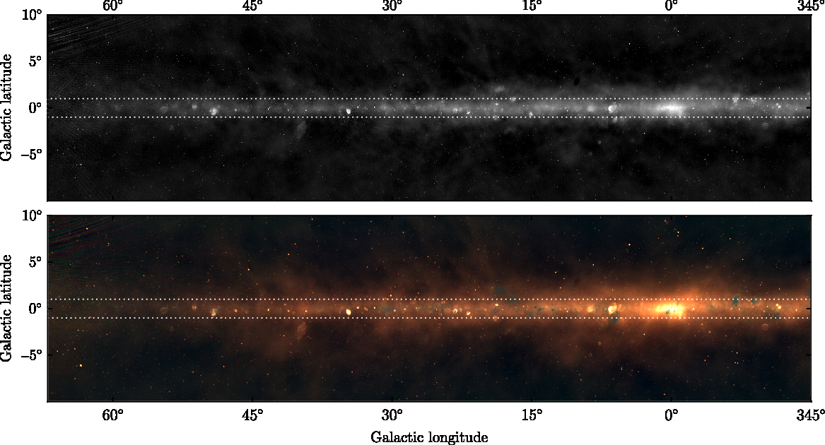
Figure 1. The wide-bandwidth images from the data described in this paper; this figure shows the iG region. The top panel shows the 170–231-MHz image which is used for source-finding (see Section 3), between -0.1 and  $5.0\,\text{Jy beam}^{-1}$, with an arcsinh stretch. The bottom panel shows an RGB cube formed of the 72–103-MHz (R), 103–134-MHz (G), and 139–170-MHz (B) data, between -1 and $10\,\text{Jy beam}^{-1}$. Dotted white lines indicate $|b|=1^\circ$; source-finding is only performed outside of this region.
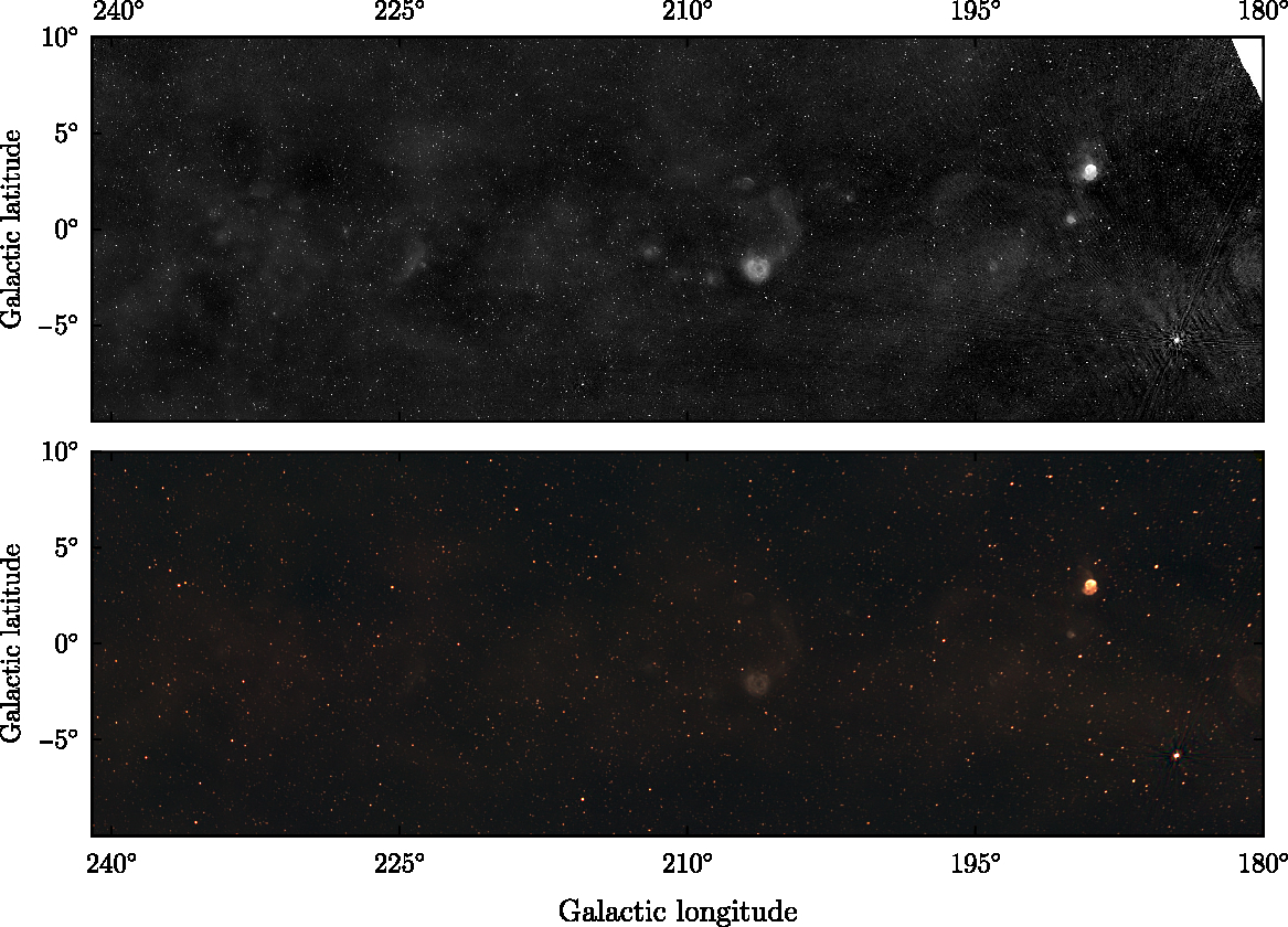
Figure 2. The wide-bandwidth images from the data described in this paper; this figure shows the oG region. The top panel shows the 170–231-MHz image which is used for source-finding (see Section 3), between –0.05 and  $1.5\,\text{Jy beam}^{-1}$, with an arcsinh stretch. The bottom panel shows an RGB cube formed of the 72–103-MHz (R), 103–134-MHz (G), and 139–170-MHz (B) data, between –0.5 and 5.0 Jy beam–1.
3. Compact source-finding
Source-finding is performed within  $1\geq|b|\leq20^\circ$ for the iG, and $|b|\leq20^\circ$ for the oG. We avoid $|b|<1^\circ$ of the iG for several reasons: the presence of bright, large-scale, galactic emission makes calculating accurate RMS and background images very difficult; the resolved emission is difficult to characterise as a set of elliptical Gaussians; and a catalogue of this region would be of limited further utility as fitted components would not often map directly to astrophysical objects, unlike compact sources, which tend to be radio galaxies, or compact galactic objects such as pulsars, PWNe, (apparently) small SNR, and H ii regions.
Following the same strategy as Hurley-Walker et al. (Reference Hurley-Walker2017), a deep wide-band catalogue centred at 200 MHz is formed, for sources with peak flux density  $\geq5\times$ the local RMS. We use the ‘priorized’ fitting technique to measure the flux densities of every detected source in the narrow-band images. The number of Gaussians allowed to form a source is limited to five, in order to prevent computationally expensive overfitting of galactic objects. We perform several checks on the quality of the catalogue, detailed in the following.
3.1. Extended sources
In total, 228 sources found during initial source-finding have a ratio of integrated to peak flux density greater than two. Visual inspection of these sources is performed and those which were components of large ( $a \gtrsim 10'$) objects are manually removed from the catalogue. These large objects are typically SNR (e.g. 3C 400.2, Milne 56), and are not included in the catalogue as, like most of the objects in the region $|b|<1^\circ$ in the iG, they cannot be easily represented as a set of elliptical Gaussians. The number of sources manually removed from the catalogue in this way is 60, leaving 168 sources with a ratio of integrated to peak flux density greater than two.
3.2. Error derivation
In this section, we examine the errors reported in the catalogue. First, we examine the systematic flux density errors; then, we examine the noise properties of the wide-band source-finding image, as this must be close to Gaussian in order for sources to be accurately characterised, and for estimates of the reliability to be made, which we do in Section 3.3. Finally, we make an assessment of the catalogue’s astrometric accuracy. These statistics are given in Table 2.
Table 2. Survey properties and statistics. We divide the survey into four parts, because the noise properties, and astrometric and flux calibration, differ slightly for each range.
3.2.1. Flux densities
The errors on the flux density measurements arise from the Dec-dependent flux density scale correction derived by Hurley-Walker et al. (Reference Hurley-Walker2017), as well as fitting errors as estimated by Aegean. As the scale correction is identical to that performed by Hurley-Walker et al. (Reference Hurley-Walker2017), we adopt the same uncertainty values of 8% for  $\mathrm{Dec} < {+}18.5^\circ$ and 13% for $\mathrm{Dec} > +18.5^\circ$. These values are listed in the catalogue for each source, and should be added in quadrature with the fitting errors when comparing with other catalogues. When fitting solely within the GLEAM catalogue, the internal flux density scale errors of 2% for $\mathrm{Dec} < +18.5^\circ$ and 3% for $\mathrm{Dec} > +18.5^\circ$ should be used (see Hurley-Walker et al. Reference Hurley-Walker2017, for a more complete discussion).
3.2.2. Astrometry
Following Hurley-Walker et al. (Reference Hurley-Walker2017), we measure the astrometry using the 200-MHz catalogue, as this provides the locations and morphologies of all sources. To determine the astrometry, unresolved ( ${(a\times b)/(a_\mathrm{PSF}\times b_\mathrm{PSF}) \lt 1.1}$), isolated (no internal match within 10’) GLEAM sources are cross-matched with similarly isolated sources in the NVSS and the Sydney University Molonglo Sky Survey (SUMSS; Bock, Large, & Sadler Reference Bock, Large and Sadler1999); the positions of sources in these catalogues are assumed to be correct, and Right Ascension (RA) and Dec offsets are measured with respect to those positions. For $\text{Dec}\le +18.{}^\circ 5$, the average RA offset is $-0.{{}^{\prime \prime }}4\pm 3.{{}^{\prime \prime }}1$, and the average Dec offset is $-1.{{}^{\prime \prime }}1\pm 3{{}^{\prime \prime }}5$. North of $+18.{{}^{{}^\circ }}5$, the average RA offset is $-0.{{}^{\prime \prime }}1\pm 2.{{}^{\prime \prime }}7$ and the average Dec offset is $1.{{}^{\prime \prime }}9\pm 3.{{}^{\prime \prime }}0$. These offsets may be somewhat different because a modified VLSSr/NVSS catalogue was used to replace MRC North of its Dec limit of 18.°5 for astrometric calibration (see Section 2.4). These offsets are all completely consistent with the values published by Hurley-Walker et al. (Reference Hurley-Walker2017) for the majority of the extragalactic sky.
In 99% of cases, fitting errors are larger than the measured average astrometric offsets. Given the scatter in the measurements, we do not attempt to make a correction for these offsets. As each snapshot has been corrected, residual errors should not vary on scales smaller than the size of the primary beam. Figure 3 shows the density distribution of the astrometric offsets, and Gaussian fits to the RA and Dec offsets, which were used to calculate the values listed in this section.
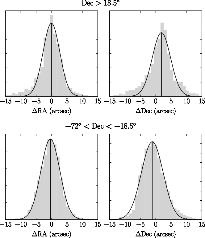
Figure 3. Histograms, weighted by source S/N, of astrometric offsets, for isolated compact GLEAM sources crossmatched with NVSS and SUMSS as described in Sectoin 3.2.2. The black curves show Gaussian fits to each histogram. Solid vertical lines indicate the mean offsets. The top panel shows sources on the northern edge of the survey  $\text{Dec}\ge +18.{{}^{{}^\circ }}5$, and the bottom panel shows sources south of this cut-off.
‘iG’ indicates the inner galactic; ‘oG’ the outer galactic region; ‘S’ indicates  $-72{}^\circ \le \text{Dec}<+18.{{}^{{}^\circ }}5$; and ‘N’ indicates $\text{Dec}\ge 18.{{}^{{}^\circ }}5$. Values are given as the mean $\pm$ the standard deviation. The statistics shown are derived from the wide-band (200 MHz) image. The flux density scale error applies to all frequencies and shows the degree to which GLEAM agrees with other published surveys. The internal flux density scale error also applies to all frequencies and shows the internal consistency of the flux density scale within GLEAM.
3.2.3. Noise properties
We briefly examine the noise properties of the wide-band (200-MHz) image. We use a  $25\,\text{deg}^2$ region covering $-10^\circ<b<-1^\circ$ with fairly typical source distribution and a background which slowly varies on ${\approx}5^\circ$ scales due to the undeconvolved large-scale side lobes of the galactic plane. Following Hurley-Walker et al. (Reference Hurley-Walker2017), we measure the background of the region using BANE and subtract it from the image. We then use AeRes from the Aegean package to mask out all sources which were detected by Aegean, down to $0.2\times$ the local RMS. Histograms of the remaining pixels are shown, for the unmasked and masked images, in Figure 4.
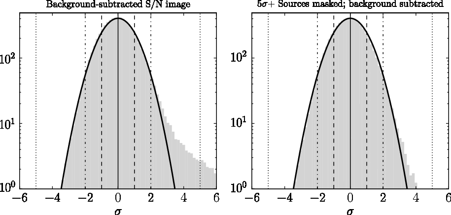
Figure 4. Noise distribution in a typical  $25\,\text{deg}^2$ of the wide-band source-finding image. BANE measures the average RMS in this region to be $24\,\text{mJy beam}^{-1}$. To show the deviation from Gaussianity, the ordinate is plotted on a log scale. The leftmost panel shows the distribution of the S/Ns of the pixels in the image produced by subtracting the background and dividing by the RMS map measured by BANE; the right panel shows the S/N distribution after masking all sources detected at $5\sigma$ down to $0.2\sigma$. The light grey histograms show the data. The black lines show Gaussians with $\sigma=1$; vertical solid lines indicate the mean values. $|\mathrm{S/N}|=1\sigma$ is shown with dashed lines, $|\mathrm{S/N}|=2\sigma$ is shown with dash-dotted lines, and $|\mathrm{S/N}|=5\sigma$ is shown with dotted lines.
The noise level in the selected region is  $\approx3\times$ higher than the RMS of the wide-band image produced for the extragalactic sky (Hurley-Walker et al. Reference Hurley-Walker2017). This is mainly due to the increased overall system temperature due to the high sky temperature. Confusion therefore forms a smaller fraction of the noise contribution, and thus the noise distribution is almost completely symmetric. For regions with lower noise, the distribution will start to skew positive, as seen by Hurley-Walker et al. (Reference Hurley-Walker2017). Noise and background maps are made available as part of the survey data release.
3.3. Completeness and reliability
Following the same procedure as Hurley-Walker et al. (Reference Hurley-Walker2017), simulations are used to quantify the completeness of the source catalogue at 200 MHz, using the wide-band mosaics. Thirty-three realisations are used in which 28 000 simulated point sources of the same flux density were injected into the 170–231 MHz mosaics, between  $1^\circ\leq|b|\leq10^\circ$. The flux density of the simulated sources is different for each realisation, spanning the range 25 mJy to 1 Jy. The positions of the simulated sources are chosen randomly but not altered between realisations; to avoid introducing an artificial factor of confusion in the simulations, simulated sources are not permitted to lie within 10’ of each other
Footnote 3
. Sources are injected into the mosaics using AeRes. The major and minor axes of the simulated sources are set to
$1^\circ\leq|b|\leq10^\circ$. The flux density of the simulated sources is different for each realisation, spanning the range 25 mJy to 1 Jy. The positions of the simulated sources are chosen randomly but not altered between realisations; to avoid introducing an artificial factor of confusion in the simulations, simulated sources are not permitted to lie within 10’ of each other
Footnote 3
. Sources are injected into the mosaics using AeRes. The major and minor axes of the simulated sources are set to  $a_\mathrm{psf}$ and $b_\mathrm{psf}$, respectively.
For each realisation, the source-finding procedures described in Section 3 are applied to the mosaics and the fraction of simulated sources recovered is calculated. In cases where a simulated source is found to lie too close to a real ( ${>}5\sigma$) source to be detected separately, the simulated source is considered to be detected if the recovered source position is closer to the simulated rather than the real source position. This type of completeness simulation therefore accounts for sources that are omitted from the source-finding process through being too close to a brighter source. In crowded regions with medium-scale features which may not be detected as discrete sources, the simulated sources are less likely to be detected, so the completeness may be underestimated in these areas, e.g. $1^\circ<|b|<2^\circ$ of the iG.
Figure 5 shows the fraction of simulated sources recovered as a function of  $S_{200\, \mathrm{MHz}}$ in the iG and oG regions of the galactic plane. For the oG, the completeness is estimated to be 50% at ${\approx} 60\,\text{mJy}$ rising to 90% at ${ox}200\,\text{mJy}$; these statistics are similar to the extragalactic catalogue (Hurley-Walker et al. Reference Hurley-Walker2017). For the iG, the completeness is considerably worse: 50% at ${\approx} 120\,\text{mJy}$ rising to 90% at ${\approx} 220\,\text{mJy}$. Errors on the completeness estimate are derived assuming Poisson errors on the number of simulated sources detected.
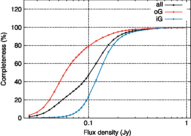
Figure 5. Estimated completeness of the catalogue for  $1{\mbox{\ensuremath{.\!^\circ}}}5<|b|<10^\circ$ as a function of $S_{200 \mathrm{MHz}}$ in the iG (blue circles), in the oG (red circles), and overall (black circles).
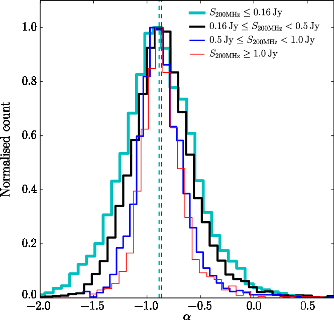
Figure 6. The spectral index distribution calculated for sources  $|b|<10^\circ$, where the fit was successful (reduced $\chi^2<1.93$). The cyan line shows sources with $S_\mathrm{200\,MHz}<0.16\,\text{Jy}$, the black line shows sources with $0.16\leq S_\mathrm{200\,MHz}<0.5\,\text{Jy}$, the blue line shows sources with $0.5\leq S_\mathrm{200\,MHz}<1.0\,\text{Jy}$, and the red line shows sources with $S_\mathrm{200\,MHz}>1.0\,\text{Jy}$. The dashed vertical lines of the same colours show the median values for each flux density cut: -0.89, -0.86, -0.88, and -0.87, respectively.
The completeness at any pixel position is given by  $C = N_{\mathrm{d}}/N_{\mathrm{s}}$, where $N_{\mathrm{s}}$ is the number of simulated sources in a circle of radius 6°
centred on the pixel and  $N_{\mathrm{d}}$ is the number of simulated sources that were detected above $5\sigma$ within this same region of sky. The completeness maps, in fits format, can be obtained from the supplementary material. Postage stamp images from the GLEAM VO server also include this completeness information in their headers.
Again using the same procedure as Hurley-Walker et al. (Reference Hurley-Walker2017), we use the same source-finding algorithm but invert the brightness, looking only for sources with  $S_\mathrm{200\,MHz}<-5\sigma$. In the $2\,670~\text{deg}^2$ region, we find 31 negative sources. As the noise distribution is close to symmetric (Section 3.2.3), we expect to see an approximately equal number of false positive sources in the same area. We thus estimate the catalogue reliability to be
 $${\rm{1}}{\rm{.0 - }}{{{\rm{31}}} \over {{\rm{22 037}}}}{\rm{ = 99}}{\rm{.86\% }}$$
3.4. Spectral fitting
Following Hurley-Walker et al. (Reference Hurley-Walker2017), we fit spectral energy distributions (following  $S\propto\nu^\alpha$) to the 20 narrow-band flux density measurements for all detected sources. We retained fit parameters only for those sources with reduced $\chi^2<1.93$, indicating a likelihood of correct fit $>99\%$ for 18 degrees of freedom.
Despite the reduced number of measurements [ $10\times$ fewer than Hurley-Walker et al. (Reference Hurley-Walker2017)], we are able to recover similar distributions of spectral indices, plotted in Figure 5. The median fitted spectral indices are slightly steeper than those of Hurley-Walker et al., even for identical flux density bins; e.g. for (high S/N) sources with $S_\mathrm{200\,MHz}>1\,\text{Jy}$, the median $\alpha$ has steepened from -0.83 to -0.89.
A potential explanation for this steepening is that pulsars, which have steep spectra of  $\alpha=-1.8\pm0.2$, make up an increasingly large fraction of our catalogue at low galactic latitudes. de Gasperin, Intema, and Frail (Reference de Gasperin, Intema and Frail2018) combined the NVSS at 1.4 GHz with the Alternative Data Release of the Tata Institute for Fundamental Research GMRT Sky Survey (TGSS-ADR1; Intema et al. Reference Intema, Jagannathan, Mooley and Frail2017) at 150 MHz to form a spectral index catalogue covering 80% of the sky. They found an excess of 86 compact and 49 non-compact steep-spectrum sources in $|b|<10^\circ$ beyond what would be expected extrapolating from the extragalactic sky.
If we restrict our search to the brightest sources where  $S_\mathrm{200\,MHz}>1.0$ Jy, of which there are 1 399 within $|b|<10^\circ$, we would need 56 to be pulsars (with $\alpha=-1.8$) to shift the median $\alpha$ from -0.83 to -0.89. However, there is only a single source that meets these criteria in our catalogue, so it appears an excess population of very steep-spectrum sources does not explain the shift in $\alpha$. Since the significance of the shift of $\alpha$ is not large compared to the inter-quartile range (IQR) of 0.22, we are unable to determine from these data alone what the cause of the steepening may be. Examining the nature of individual sources by comparison with other data at other frequencies will likely reveal whether the shift is astrophysical or some as-yet uncharacterised systematic.
3.4.1. Comparison with extragalactic catalogue
Having reprocessed all data within  $|b|<20^\circ$, there exists an overlap with the extragalactic catalogue of Hurley-Walker et al. (Reference Hurley-Walker2017), for the range $10{^{\circ}}<|b|<20{^{\circ}}$. We can use this overlap to check for flux density scale consistency between the two catalogues. Figure 7 shows a comparison of three major attributes between the catalogues: the integrated flux density in the 170–231 MHz wide-band images, the fitted 200 MHz flux density over all frequency bands, and the fitted spectral index $\alpha$ over all frequency bands.
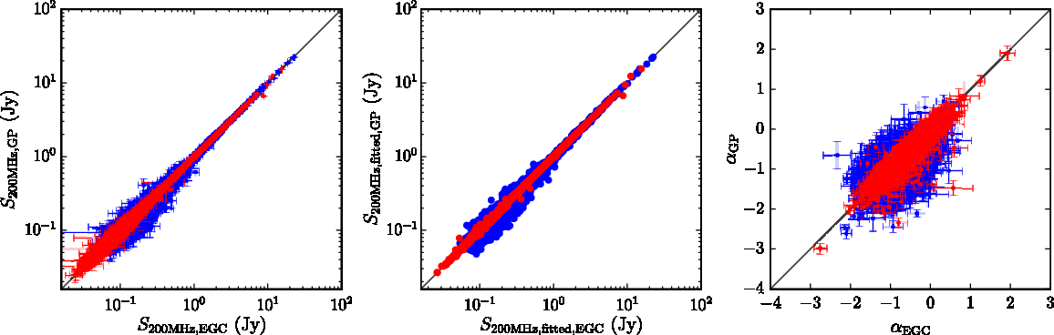
Figure 7. Three comparisons of the galactic plane catalogue (ordinates) with the extragalactic catalogue (abscissae). The left panel shows the integrated flux densities measured at 200 MHz in the wide-band mosaics, with error bars indicating only the fitting errors produced by Aegean. The middle panel shows the fitted 200-MHz flux densities over all 20 flux density measurements (see Section 3.4); error bars are not shown as they become very large on a log scale at low flux densities. The right panel shows the fitted  $\alpha$. Red points are from the oG region (in which no additional data reduction was performed) and blue points indicate the iG region (which was completely reprocessed using more observations and multiscale CLEAN).
No biases or trends are visible; the catalogues are on the same flux density scales. There is a larger amount of scatter on the iG points, likely due to the increased number of observations used to generate the mosaics, and the slightly different processing scheme. As expected, there is very little scatter on the oG points, since the results of this source-finding are essentially the same as the measurements made by Hurley-Walker et al. (Reference Hurley-Walker2017). Differences mainly arise in the range  $b<-10^\circ$ for the oG, where a different set of mosaics was originally used by Hurley-Walker et al. (Reference Hurley-Walker2017) to generate the catalogue for that area of sky.
3.5. Final catalogue
Having established the quality of the catalogue, we filter it to retain only  $|b|\leq10^\circ$, in order not to duplicate existing results. The resulting catalogue consists of 22 037 radio sources detected over $2\,670~\text{deg}^2$. Of these, 5 749 sources are resolved (ratio of integrated to peak flux density >1.1); just 168 sources are appreciably extended (ratio of integrated to peak flux density >2.0). Here 17 244 sources are fit well by power-law spectral energy distributions (SEDs). The catalogue has 311 columns identical to those in Appendix A of Hurley-Walker et al. (Reference Hurley-Walker2017) and is available via Vizier.
The catalogue measurements can be used to perform more complex spectral fits, especially in conjunction with other radio measurements. Figure 8 shows four example curved fits across GLEAM and data from the literature for two peaked-spectrum sources, a planetary nebula, and a pulsar.
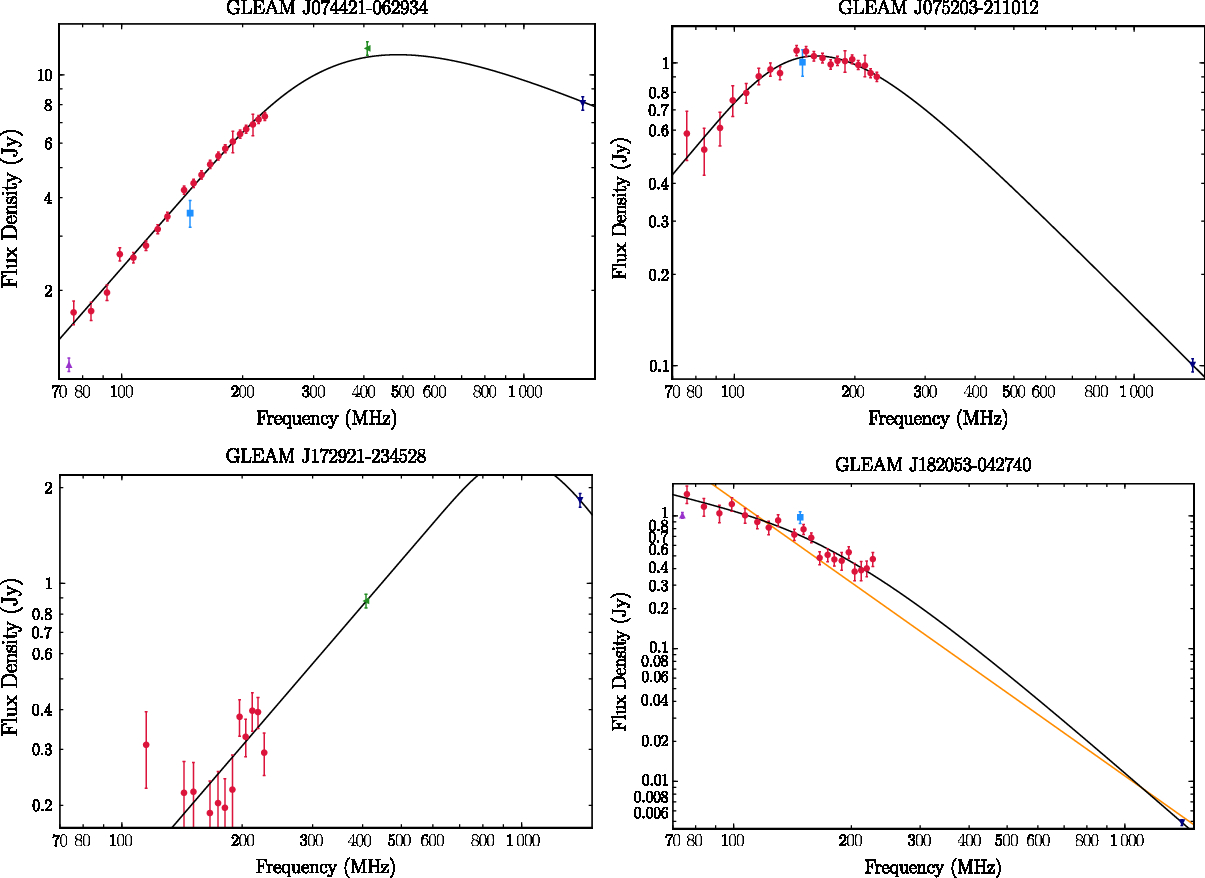
Figure 8. Four-example curved spectral energy distributions fit (black lines) to the narrow-band GLEAM measurements (red circles) and, where available, VLSSr (purple upward-pointing triangle), TGSS-ADR1 (light blue square), MRC (green leftward-pointing triangle), and NVSS (dark blue downward-pointing triangle), with fitting performed as by Callingham et al. (Reference Callingham2015). The yellow line in the bottom-right panel shows a simple power-law SED fit. Sources shown are, from top-left to bottom-right, the known peaked-spectrum source  $4\text{C}\,-06.18$ (Davis Reference Davis1967), a previously unknown peaked-spectrum source, the planetary nebula NGC 6369 (Curtis Reference Curtis1918), and the pulsar J1820-0427 (Vaughan, Large, & Wielebinski Reference Vaughan, Large and Wielebinski1969).
4. Galactic plane
Utilising the large number of short baselines in the Phase I configuration of the MWA, GLEAM has sensitivity to structures on large scales. The shortest baseline in the array is 7.72 m in length, allowing access to angular scales of $ <29^\circ$ at 76 MHz, or $<10^\circ$ at 227 MHz. Objects smaller than this should have correct flux densities across all frequencies. However, an important quantity which also changes with frequency is the background to any object to be measured, and this will also change rapidly with frequency due to the intrinsic synchrotron spectrum of the diffuse background ( $T\propto\nu^{-2.7}$) and the aforementioned resolution effects. The PSF will also change as a function of $\nu$, and is provided in the header in any postage stamp downloaded from the GLEAM VO server. We thus urge the reader to be careful of these effects when measuring flux densities in the images.
As visible in Figures 1 and 2, these images contain a wealth of data on galactic objects. Figure 9 shows the discriminating power of the wide bandwidth in examining the physical origin of different kinds of emission. In the case of the Moon (top left panel), the disc obscures the background galactic synchrotron emission and reflects the FM radio emitted by the Earth, giving the centre a red appearance. The top right panel shows the known H ii region  $\text{G}6.165-1.168$ (Lockman Reference Lockman1989) and the known SNR ‘Milne 56’ (Clark, Green, & Caswell Reference Clark, Green and Caswell1975); free-free absorption and thermal emission gives the H ii region a distinctive blue appearance (positive $\alpha$) while the SNR has a fairly flat spectral index of -0.2 and appears slightly orange against the red of the steep-spectrum diffuse galactic synchrotron. The lowest panel of Figure 9 shows the GLEAM view of the galactic centre, with strong free-free absorption and an intriguing loop of absorption perpendicular to the galactic plane (Anderson et al., in preparation).
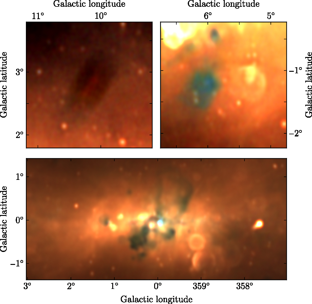
Figure 9. Three example images from this galactic plane data release, using an RGB cube formed of the 72–103-MHz (R), 103–134-MHz (G), and 139–170-MHz (B) data. The top left panel shows the Moon averaged over approximately 1 h of observing; the top right panel shows on a known H ii region (left) and a known SNR (right); the bottom panel shows a view of the galactic centre. The colour ranges used are -0.1–4, -0.1–5, and  $-0.5-20\,\text{Jy beam}^{-1}$ for each panel, respectively.
Some studies have already been published using these data: Su et al. (Reference Su2017); Su et al. (Reference Su2018) used the low-frequency absorbing properties of H ii regions to measure the cosmic ray emissivity of the galactic plane along those lines of sight, Su et al. (in preparation) produce a catalogue of all H ii regions selected from this region; Maxted et al. (submitted) examine in detail the  $\gamma$-ray and radio properties of the young SNR $\text{G}\,23.11+0.18$; Hurley-Walker et al. (submitted) characterise 19 SNR candidates from the literature, including discriminating H ii regions from SNR candidates; and Hurley-Walker et al. (submitted) discover 27 SNRs, 6 with pulsar associations.
There remain many interesting features in these data, and the field is open to compare them with other recently published surveys of the galactic plane, such as the gamma-ray survey of H.E.S.S. Collaboration et al. (Reference Collaboration2018) and the wide-band infrared survey of Wright et al. (Reference Wright2010). All images are available via the GLEAM VO server Footnote 4 and SkyView. Footnote 5
5. Conclusions
This work makes available a further  $2\,860~\text{deg}^2$ of the GLEAM survey, using multi-scale CLEANing to better deconvolve large-scale galactic structure. For the latitude ranges $345^\circ < l < 67^\circ$, $180^\circ < l < 240^\circ$, we provide images covering $|b|<10^\circ$; for the latter longitude range we also provide a compact source catalogue, while for the longitude range towards the galactic centre, we provide a compact source catalogue over $1^\circ\leq|b|\leq10^\circ$; the catalogue consists of 22 037 sources in total.
Acknowledgements
We thank the anonymous referee for their comments, which improved the quality of this paper. This scientific work makes use of the Murchison Radio-astronomy Observatory, operated by CSIRO. We acknowledge the Wajarri Yamatji people as the traditional owners of the Observatory site. Support for the operation of the MWA is provided by the Australian Government (NCRIS), under a contract to Curtin University administered by Astronomy Australia Limited. We acknowledge the Pawsey Supercomputing Centre, which is supported by the Western Australian and Australian Governments. The National Radio Astronomy Observatory is a facility of the National Science Foundation operated under cooperative agreement by Associated Universities, Inc. We acknowledge the work and support of the developers of the following python packages: Astropy (The Astropy Collaboration et al. 2013), Numpy (van der Walt, Colbert, & Varoquaux Reference van der Walt, Colbert and Varoquaux2011), and Scipy (Jones et al. Reference Jones2001). We also made extensive use of the visualisation and analysis packages DS9 Footnote 6 and Topcat (Taylor 2005). This work was compiled in the very useful free online LaTeX editor Overleaf.


