


1. Introduction
Combustion noise is central to efforts to curb aircraft emissions. Noise originating in the combustor is an important contributor to overall aircraft noise, particularly during approach and landing phases. Further, combustion-generated sound can act as a source of thermoacoustic instabilities, the consequences of which may range from decreased efficiency to system failure (Lieuwen Reference Lieuwen2003). Modern lean-premixed systems designed to lower  $\textrm {NO}_{x}$ emissions can be particularly susceptible to this phenomenon (Dowling & Mahmoudi Reference Dowling and Mahmoudi2015). In this sense, developing a thorough understanding of the sources of combustion noise is an important step in view of meeting increasingly strict emission targets.
In the present work, we use the word noise to indicate any pressure fluctuation propagating inside or outside the system. A distinction is usually drawn between direct and indirect combustion noise (Dowling & Mahmoudi Reference Dowling and Mahmoudi2015). Direct noise results from the volumetric expansion and contraction brought about by unsteady heat release in the combustion zone. Indirect noise is generated when perturbations in the temperature, composition or vorticity generated within the combustion zone are accelerated/decelerated, creating acoustic waves. In a gas turbine, indirect noise is produced at the nozzle or turbine guide vanes, and propagates both downstream, where it contributes to overall aircraft noise (Dowling & Mahmoudi Reference Dowling and Mahmoudi2015), and upstream into the combustor, where it may lead to the onset of thermoacoustic instabilities (Polifke, Paschereit & Dobbeling Reference Polifke, Paschereit and Dobbeling2001; Goh & Morgans Reference Goh and Morgans2013; Morgans & Duran Reference Morgans and Duran2016).
Entropy noise associated with temperature fluctuations has been the topic of numerous studies since it was theorised in the 1960s (Cuadra Reference Cuadra1967). Marble & Candel (Reference Marble and Candel1977) obtained one-dimensional transfer functions for the noise generated at an isentropic compact nozzle for a low-frequency impinging entropic perturbation, in subsonic and supersonic conditions, with and without a shock in the diffuser for the supersonic case. These transfer functions were later extended to finite length nozzles for arbitrary frequencies (Goh & Morgans Reference Goh and Morgans2011; Duran & Moreau Reference Duran and Moreau2013). In the supersonic case, the entropic indirect noise generation was analysed in detail by Moase, Brear & Manzie (Reference Moase, Brear and Manzie2007) and Leyko et al. (Reference Leyko, Moreau, Nicoud and Poinsot2011), while the interaction of entropy spots with two-dimensional shock waves was studied in detail by Mahesh, Lele & Moin (Reference Mahesh, Lele and Moin1997) and Farag, Boivin & Sagaut (Reference Farag, Boivin and Sagaut2019).
In parallel to these developments, Magri, O'Brien & Ihme (Reference Magri, O'Brien and Ihme2016) and Ihme (Reference Ihme2017) developed transfer functions for the indirect noise generated at a compact nozzle due to compositional perturbations, which was generalised to non-compact nozzles in subsonic and supersonic conditions in Magri (Reference Magri2017). Further numerical investigations have shown the relative importance of the compositional mechanism relative to temperature fluctuations in a realistic rich-quench-lean combustor (Giusti, Magri & Zedda Reference Giusti, Magri and Zedda2019).
This range of theoretical and numerical studies on noise generation from temperature and composition fluctuations has spurred a number of simplified validation experiments involving the conversion of temperature and compositional disturbances into acoustic noise. In the Entropy Wave Generator (EWG) developed at Deutsches Zentrum für Luft- und Raumfahrt (DLR), entropic waves were generated in a duct using an electric heater, accelerated through a subsonic or supersonic nozzle, and the resulting pressure trace was measured further downstream of the nozzle (Bake et al. Reference Bake, Richter, Mühlbauer, Kings, Röhle, Thiele and Noll2009). In those experiments, the upstream-propagating entropy noise was not measured, even though it may play a role in thermoacoustic instabilities (Polifke et al. Reference Polifke, Paschereit and Dobbeling2001; Goh & Morgans Reference Goh and Morgans2013). Following this effort, several model experiments were developed to validate entropic indirect noise generated in convergent–divergent nozzles (Knobloch et al. Reference Knobloch, Lahiri, Enghardt, Bake and Peitsch2011; Gaetani, Persico & Spinelli Reference Gaetani, Persico and Spinelli2015; Tao et al. Reference Tao, Schuller, Huet and Richecoeur2017). Experiments conducted on the Cambridge Entropy Generator Rig focused on the upstream-propagating indirect noise (De Domenico, Rolland & Hochgreb Reference De Domenico, Rolland and Hochgreb2017). By accounting for direct noise and acoustic reflections, the indirect noise could be clearly identified and isolated in the acquired pressure traces (Rolland, De Domenico & Hochgreb Reference Rolland, De Domenico and Hochgreb2017). De Domenico, Rolland & Hochgreb (Reference De Domenico, Rolland and Hochgreb2019a) extended the compact model to non-isentropic subsonic nozzles in which entropy in the mean flow is not conserved, i.e. nozzles with pressure losses occurring in the divergent section. It was found that the non-isentropicity of a system significantly affects indirect noise generation. More recently, Rolland, De Domenico & Hochgreb (Reference Rolland, De Domenico and Hochgreb2018) used a mass injection device to validate a one-dimensional model for generation of compositional indirect noise in choked isentropic nozzles, focusing on the behaviour of upstream-propagating waves. The latter work did not consider the consequences of the non-isentropicity of the nozzles on the generation of compositional noise, nor the behaviour of downstream travelling waves. The present work tackles these two specific issues. We combine the techniques used for generation and identification of compositional noise developed by Rolland et al. (Reference Rolland, De Domenico and Hochgreb2018) with the extension of the treatment of non-isentropic nozzles in De Domenico et al. (Reference De Domenico, Rolland and Hochgreb2019a) to provide experimental validation of the theory for compositional noise in non-isentropic nozzles operating in subsonic-to-sonic throat conditions. The opportunity for validation under these operating conditions provides a solid foundation for the determination of the contribution of compositional and thermal indirect noise to both instabilities inside combustion chambers, as well as noise propagation downstream through nozzle guide vanes.
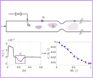
In the present experiments, we measure the entropic and compositional noise generated by the injection of pockets of helium, argon, carbon dioxide and methane into a mean flow of air, which is accelerated through non-isentropic nozzles. The indirect noise model proposed by De Domenico et al. (Reference De Domenico, Rolland and Hochgreb2019a) for entropy noise in non-isentropic nozzles is extended to include compositional noise. Measurements are obtained in subsonic-to-sonic throat conditions for low-frequency perturbations. Both the upstream- and downstream-propagating components of the indirect noise are resolved using a source identification technique based on the reverberation of sound waves in an enclosed chamber.
The paper is organised as follows. One-dimensional models for the generation of direct and indirect acoustic waves in flow ducts are presented in § 2. The effect of acoustic reflections (reverberation) of these waves is modelled in § 3 to develop a source identification method. Experiments are conducted on the Cambridge Entropy Wave Generator described in § 4, where direct, entropic and compositional noise is generated by injecting pockets of helium, argon, carbon dioxide or methane into a flow of air. The corresponding experimental pressure measurements are shown in § 5. Source and system identification is performed to clearly identify and isolate direct and indirect noise. These results are finally compared to simulations carried out with the predictions of the proposed physics-based low-order model for non-isentropic nozzle transfer functions.
2. Direct and indirect noise generation
In this work, we consider a multi-component ideal gas mixture flowing in a chamber terminated with a nozzle. We assume a quasi-one-dimensional framework: the flow variables change because of area variations and are assumed to be uniform across the duct cross-section, so the nozzle flow depends only on the axial coordinate. The gas is chemically frozen, which corresponds to a combustor situation in which the reaction process is completed upstream of the nozzle guide vanes, yet compositional fluctuations (e.g. equivalence ratio fluctuations) are generated. The flow is assumed to be advection dominated, so that viscosity, heat/species diffusivity and body forces are negligible. The multi-component gas is composed of  $N$ species with mass fraction
  $Y_i$, molecular weight
  $W_i$ and chemical potentials
  $\mu _i$. All species are expressed in terms of mixture fraction
  $Z$, so that
  $Y_i = Y_i(Z)$, and have frozen internal energy modes, so the heat capacity only depends on the mixture composition. The conservation of mass, momentum, energy and species in their differential form read, respectively (e.g. Chiu & Summerfield Reference Chiu and Summerfield1974; Magri Reference Magri2019)
 \begin{equation} \left. \begin{gathered} \dfrac{\textrm{D} \rho}{\textrm{D} t} + \rho \dfrac{\partial u }{\partial x} = \dot{S}_{m}, \\ \rho \dfrac{\textrm{D} u}{\textrm{D} t} + \dfrac{\partial p }{\partial x} = \dot{S}_{M},\\ T \dfrac{\textrm{D} s}{\textrm{D} t} + \sum_{i=1}^{N} \dfrac{\mu_i}{W_i}\dfrac{\textrm{D}Y_i}{\textrm{D}t} = \dot{S}_{s},\\ \rho \dfrac{\textrm{D}Y_i}{\textrm{D}t} = \dot{S}_i, \end{gathered} \right\} \end{equation}
where  $x$ and
  $t$ are the spatial and temporal coordinates, respectively;
  $\rho$,
  $p$ ,
$p$ ,  $T$,
$T$,  $u$,
$u$,  $s$,
$s$,  $Y_i$,
  $\mu _i$ and
  $W_i$ are the local fluid density, pressure, temperature, velocity, entropy, mass fraction, chemical potential and molar fraction, respectively. The subscript
  $i$ denotes the
  $i$th species. The right-hand side source terms
  $\dot {S}_{j}$ are the local rates of change of mass, momentum, energy and species, respectively.
The direct and indirect noise generation processes are described by applying linear perturbations to the conservation equations (2.1) (Marble & Candel Reference Marble and Candel1977; Duran, Moreau & Poinsot Reference Duran, Moreau and Poinsot2013; Magri Reference Magri2017). The unsteady source generates direct noise, in the form of forward- and backward-propagating acoustic waves,  ${\rm \pi} _d^+$ and
  ${\rm \pi} _d^-$, respectively (figure 1), entropic waves
  $\sigma$ and compositional waves
  $\xi$. The waves manifest themselves as fluctuations in the flow variables, which can be decomposed into their mean and fluctuating components (denoted with an overbar and a prime, respectively: e.g.
  $p(x,t) = \bar {p}(x) + p'(x,t)$). Furthermore, we consider linear perturbations, so that their amplitude is negligible with respect to the mean quantity (i.e.
  $p' \ll \bar {p}$). The four waves in the experiments correspond to the downstream- and upstream-propagating acoustic waves
  ${\rm \pi} ^{\pm }$ generated by the unsteady injection of the secondary flow, the convective entropy wave
  $\sigma$ and the convective compositional wave
  $\xi$. These waves are defined as (Magri et al. Reference Magri, O'Brien and Ihme2016):
 \begin{equation} {\rm \pi}^{\pm} \equiv \frac{1}{2} \left( \frac{ p'}{\bar{\gamma} \bar{p} } \pm \frac{ u'}{\bar{c}} \right), \quad \sigma \equiv \frac{ s'}{\bar{c}_p}, \quad \xi \equiv Z', \end{equation}
where  $\bar {c}_p$ is the heat capacity of the flow,
  $\bar {\gamma }$ the specific heat capacity ratio and
  $\bar {c}$ is the speed of sound. Linearising the ideal gas law gives
  $p'/\bar {p} = \rho '/ \bar {\rho } +R'/ \bar {R} +T'/ \bar {T}$, where
  $R$ is the gas constant of the mixture. The Gibbs equation for calorically perfect multi-component gas is
 \begin{equation} \sigma = \frac{ s'}{\bar{c}_p} = \frac{p'}{\bar{\gamma} \bar{p}}-\frac{\rho'}{\bar{\rho}} { + \frac{c_p'}{\bar{c}_p} -\frac{R'}{\bar{R}}} - \frac{1}{\bar{c}_p\bar{T}} \sum_{i=1}^{N} \frac{\mu_i}{W_i}\,\textrm{d}Y_i. \end{equation}
Following Magri (Reference Magri2017), we define the chemical potential  $\varPsi$ and the heat-capacity factor
  $\aleph$ as
 \begin{gather} \varPsi = \frac{1}{\bar{c}_p\bar{T}} \sum_{i=1}^{N} \left(\frac{\mu_i}{W_i} \right) \frac{\textrm{d}Y_i}{\textrm{d}Z}, \end{gather}
 \begin{gather} {\aleph = \frac{R'}{\bar{R}} - \frac{c_p'}{\bar{c}_p} = \sum_{i=1}^{N} \left(\frac{1}{\bar{R}}\frac{\textrm{d} \bar{R}}{\textrm{d}Y_i} - \frac{1}{\bar{c}_p}\frac{\textrm{d} \bar{c}_p}{\textrm{d}Y_i} \right ) \frac{\textrm{d}Y_i}{\textrm{d}Z}}. \end{gather}
Figure 1. Direct acoustic ( ${\rm \pi} ^-_d$,
  ${\rm \pi} ^+_d$), entropic (
 $\sigma$) and compositional (
 $\xi$) waves produced at a wave generator, and indirect acoustic waves (
 ${\rm \pi} ^-_{\sigma }$,
  ${\rm \pi} ^-_{\xi }$,
  ${\rm \pi} ^+_{\sigma }$ and
  ${\rm \pi} ^+_{\xi }$) generated by the acceleration of entropic and compositional disturbances at a nozzle further downstream.
From (2.4) and (2.5), the entropy wave  $\sigma$ from (2.3) can be briefly expressed as
 \begin{equation} \sigma = \frac{p'}{\bar{\gamma}\bar{p}} - \frac{\rho'}{\bar{\rho}} - (\aleph + \psi) \xi. \end{equation}
This shows that the entropic and compositional waves are coupled, since the specific entropy is related to the local gas composition.
After being generated at the source, the entropic and compositional waves are convected with the flow downstream of the source towards the nozzle. When accelerated, they generate forward and backward entropic–acoustic waves  ${\rm \pi} ^+_{\sigma }$ and
  ${\rm \pi} ^-_{\sigma }$ and compositional–acoustic waves
  ${\rm \pi} ^+_{\xi }$ and
  ${\rm \pi} ^-_{\xi }$, as shown in figure 1. The nozzle length
  $L_n$ is short compared to the acoustic wavelengths of the experiment
  $\lambda$ (
 $L_n / \lambda < 0.01$). Therefore, the nozzle is assumed to be compact, which means that the flow variables of the approaching and discharging flow are related by algebraic jump conditions. The transversal waves can also be neglected, as the characteristic frequencies of circumferential modes,
  $f_{circ} = ({4{\rm \pi} c}/{d}) (1-M^2)^{-1/2} \approx 10^5\ \textrm {Hz}$ (where
  $d$ is the diameter of the duct and
  $M$ the Mach number) are much higher than the characteristic frequencies of the injection,
  $f_{inj} \simeq 1\text{--}10 \ {\rm Hz}$ and of the longitudinal acoustic modes,
  $f_{long} \simeq 100\ \textrm {Hz}$.
2.1. Jump conditions across a wave generator
The conventional definition of direct noise in a combustion system is associated with the pressure fluctuations produced by a flame due to the unsteady heat flux. Here, by direct noise we indicate the sound generated in a non-reacting environment by a wave generator that produces unsteady perturbations in the mass, momentum and energy fluxes, as well as in the mixture fraction. This simplified formulation allows us to examine the effect of unsteady heat addition by a heating grid in a flow (working principle for the DLR and Cambridge EWG (Bake et al. Reference Bake, Richter, Mühlbauer, Kings, Röhle, Thiele and Noll2009; De Domenico et al. Reference De Domenico, Rolland and Hochgreb2017)) and the effect of fluid injection (Rolland et al. Reference Rolland, De Domenico and Hochgreb2018), which is of particular interest for the experiments in the Cambridge Entropy Wave Generator with mass addition, as well as for realistic modelling of the effects of cooling or secondary air injection in combustors.
In order to capture the effect of the wave generator on the flow variables, jump conditions are applied, whereby mass, momentum, energy and mixture fraction fluxes ( $\phi _m$,
  $\phi _M$,
  $\phi _e$ and
  $\phi _Z$, respectively) are added to the flow at a discontinuity. The generator compactness is an appropriate assumption because the length of the wave generators in the experiments is small relative to the wavelengths of interest (i.e. low frequency waves (De Domenico et al. Reference De Domenico, Rolland and Hochgreb2017)). This situation is depicted in figure 2. In addition, we assume that the magnitudes of these fluxes have small value relatively to the mean flow values (
 $\bar {\phi }=0$,
  $\phi =\phi '$). The mean flow properties are assumed to be conserved across the discontinuity. Using the one-dimensional conservation equations for mass, momentum, energy and species, the flow perturbations on either side of the discontinuity can be related to the added fluxes
  $\phi _m'$,
  $\phi _M'$,
  $\phi _e'$ and
  $\phi _Z'$
 \begin{equation} \left. \begin{gathered} \left[\dot{m}'\right]^1_0 = \phi'_m, \\ \left[\left( p + \rho u^2 \right)' \right]^1 _0 = \phi'_M, \\ \left[\left(\rho u \left({c_p} T + \tfrac{1}{2}u^2\right)\right)' \right]^1 _0 = \phi'_e, \\ \left[Z' \right]^1 _0 = \phi'_Z. \end{gathered} \right\} \end{equation}
The notation  $[ \bullet ]_0^1$ denotes the difference between the flow variables immediately upstream
  $[0]$ and downstream
  $[1]$ of the discontinuity, such that
  $[\bullet ]_0^1 =(\bullet )_1 -(\bullet )_0$. Normalising (2.7) results in the following perturbation equations:
 \begin{equation} \left. \begin{gathered} \left[\left(\dfrac{\rho'}{\bar{\rho }}\right) + \dfrac{1}{\bar{M}} \left(\dfrac{u'}{\bar{c}}\right) \right] ^1 _0 = \varphi'_m,\\ \left[\dfrac{1}{\bar{M}^2}\left(\dfrac{p'}{\bar{\gamma} \bar{p}}\right) + \left(\dfrac{\rho'}{\bar{\rho }}\right) + \dfrac{2}{\bar{M}} \left(\dfrac{u'}{\bar{c}}\right) \right]^1 _0 = \varphi'_M,\\ \left[\dfrac{\rho'}{\bar{\rho }} + \dfrac{1}{\bar{M}} \dfrac{u'}{\bar{c}} +\dfrac{1}{1+\displaystyle \frac{\bar{\gamma}-1}{2}\bar{M}^2} \left ( \bar{\gamma} \dfrac{p'}{\bar{\gamma} \bar{p}} - \dfrac{\rho'}{\bar{\rho}} +(\bar{\gamma} - 1)\bar{M} \dfrac{u'}{\bar{c}} -\aleph \xi \right) \right]^1 _0 = \varphi'_e,\\ \left[Z' \right]^1 _0 = \varphi'_Z, \end{gathered} \right\} \end{equation}
where  $\bar {M}$ is the Mach number, and
  $\varphi '_m$,
  $\varphi '_M$,
  $\varphi '_e$ and
  $\varphi '_Z$ are the normalised changes in mass, momentum, energy and mixture fraction, respectively:
 \begin{equation} \varphi'_m=\frac{\phi'_m}{\bar{\rho} \bar{u}}, \quad \varphi'_M=\frac{\phi'_M}{\bar{\rho} \bar{u}^2}, \quad \varphi'_e=\frac{\phi'_e}{\bar{\rho} \bar{u} \bar{c}_p \bar{T}_T}, \quad \varphi'_Z={\phi'_Z}. \end{equation}
where  $\bar{T}_T$ is the total temperature. The injection generates acoustic, entropic and compositional waves, whose amplitude can be computed by substituting the flow variables (2.8) with their definitions (2.2), as shown in appendix A. In the scenario where there are no incoming waves (
 ${{\rm \pi} ^+_0={\rm \pi} ^-_1=\sigma _0=\xi _0=0}$ in figure 2), the discontinuity generates forward- and backward-propagating acoustic waves
  ${\rm \pi} _{d}^+={\rm \pi} _1^+$ and
  ${\rm \pi} _{d}^-={\rm \pi} _0^-$ (direct noise), as well as forward-propagating entropic and compositional waves
  $\sigma =\sigma _1$ and
  $\xi =\xi _1$.
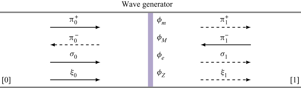
Figure 2. Forward and backward acoustic ( ${\rm \pi} ^+$,
  ${\rm \pi} ^-$), entropic waves
  $\sigma$ and compositional waves
  $\xi$ upstream
  $[0]$ and downstream
  $[1]$ of a wave generator. Impinging waves (black solid line) and generated waves (black dashed line).
From (2.8), the entropy wave  $\sigma$ and compositional wave
  $\xi$ generated at the discontinuity can be expressed as
 \begin{equation} \sigma =(\varphi'_e - \varphi'_m) + \frac{(\bar{\gamma} -1)}{2}{\bar{M}^2} \left(\varphi'_m - 2 \varphi'_M + \varphi'_e \right) - \varPsi \varphi'_Z, \quad \xi=\varphi'_Z. \end{equation}
Equation (2.10) shows that the production of an entropic wave is driven by three physical mechanisms. First, entropy is generated if there is a mismatch between the energy and mass perturbations (if  $\varphi '_e \neq \varphi '_m$). This is physically intuitive: if energy is added with no mass to carry it, the local specific entropy increases. Second, if energy is carried with the corresponding mass, but without a matching momentum perturbation
  $\varphi '_M$, entropy is generated. Third, changes in the flow composition
  $\varphi '_Z$ can modify the entropy: this is because the gases composing the mixture may have different entropy relatively to the main mixture. Finally, the addition of a compositional flux
  $\varphi '_Z$ leads to the generation of a compositional wave. If there is no mass, momentum and composition sources, and only energy is added to the flow, the situation simplifies to the case of an unsteady heat source
  $q'=\varphi '_e$ (Bake et al. Reference Bake, Richter, Mühlbauer, Kings, Röhle, Thiele and Noll2009; De Domenico et al. Reference De Domenico, Rolland and Hochgreb2017) and the model derived above then reduces to the one previously used for the EWG (Leyko, Nicoud & Poinsot Reference Leyko, Nicoud and Poinsot2009; Duran et al. Reference Duran, Moreau and Poinsot2013).
2.2. Transfer functions for a subsonic-to-sonic compact nozzle
Indirect noise is generated when entropic or compositional convected inhomogeneities are accelerated or decelerated, as when they pass through nozzles or turbine blades. The total upstream and downstream-propagating indirect noise  ${{\rm \pi} _i^-}$ and
  ${{\rm \pi} _i^+}$ waves are a combination of the entropic
  ${\rm \pi} _{\sigma }$ and compositional noise
  ${\rm \pi} _{\xi }$:
  ${{{\rm \pi} _i^-}= ({{\rm \pi} _{\xi }^-}/{\xi }) {\xi } + ({{\rm \pi} _{\sigma }^-}/{\sigma }) {\sigma }}$ and
  ${{{\rm \pi} _i^+}= ({{\rm \pi} _{\xi }^+}/{\xi }) {\xi } + ({{\rm \pi} _{\sigma }^+}/{\sigma }) {\sigma }}$. Marble & Candel (Reference Marble and Candel1977) and Magri et al. (Reference Magri, O'Brien and Ihme2016) considered the case of a subsonic isentropic nozzle and that of a supersonic nozzle with a shock in the divergent section, where the total entropy losses are localised. Viscous effects are considered to be negligible, so the flow in the nozzle is modelled as inviscid. The nozzle length is much smaller than the wavelength of the disturbances, so the nozzle is assumed to be compact. The boundary layer thickness decreases in the accelerating flow in the converging section, which means that viscous losses are small. Under these isentropic conditions, the conservation equations can be formulated as a set of jump conditions, which relate the flow variables upstream and downstream of the convergent nozzle, as follows:
 \begin{equation} \left. \begin{gathered} \left[ \dot{m} \right]^2 _1 = 0, \\ \left[ T_T \right]^2 _1 = 0, \\ \left[ s \right]^2 _1 = 0, \\ \left[ Z \right]^2 _1 = 0 . \end{gathered} \right\} \end{equation}
One of the main assumptions in the prior work (Marble & Candel Reference Marble and Candel1977; Magri et al. Reference Magri, O'Brien and Ihme2016; Magri Reference Magri2017) is that the flow inside the nozzle is entirely isentropic, i.e. reversible and adiabatic (apart from an eventual shock in the divergent section). In reality, pressure losses and flow recirculation may occur, especially in the diverging part of the nozzle, where the pressure gradient is adverse to the flow velocity, so that entropy is not conserved i.e. the flow is non-isentropic. These effects are included in the model of non-isentropic orifice plates (similarly to previous work by Bechert (Reference Bechert1980) and Durrieu et al. (Reference Durrieu, Hofmans, Ajello, Boot, Auregan, Hirschberg and Peters2001), where turbulence is generated after the throat). De Domenico et al. (Reference De Domenico, Rolland and Hochgreb2019a) introduced a model for describing the quasi-steady transfer functions of non-isentropic compact nozzles with subsonic-to-sonic throat conditions, a diagram of which is shown in figure 3.

Figure 3. Diagram of the flow areas at the inlet ( $A_1$), throat (
 $A_t$), jet location (
 $A_j$) and outlet (
 $A_2$) of a non-isentropic nozzle, with streamlines for illustration.
The nozzle modelled by De Domenico et al. (Reference De Domenico, Rolland and Hochgreb2019a) is defined by the cross-sections at the inlet  $A_1$, throat
  $A_t$ and outlet area
  $A_2$. The nozzle is modelled as compact (i.e. low-frequency perturbations) so that the shape of the nozzle between these cross-sections is immaterial. The converging part of the nozzle is modelled as isentropic regardless of the shape of the converging section (Durrieu et al. Reference Durrieu, Hofmans, Ajello, Boot, Auregan, Hirschberg and Peters2001; Dowling & Stow Reference Dowling and Stow2003): the assumption of isentropicity is justified for sufficiently large Reynolds numbers, and for converging flows. Viscous effects are important, particularly near the throat of the nozzle. This is taken into account by a vena contracta factor,
  $\varGamma < 1$, such that the minimum area of the throat
  $A_{min}$ is smaller than the geometric throat area,
  $A_t$. In the divergent section, losses and recirculation might occur due to the adverse pressure gradient. Depending on the nozzle and flow characteristics, the flow can behave somewhere between isentropic and non-isentropic. This was modelled by defining an effective jet mixing area
  $A_j$, assuming that the flow is isentropic from
  $A_t$ to
  $A_j$, and that a non-isentropic jet (Bechert Reference Bechert1980; Durrieu et al. Reference Durrieu, Hofmans, Ajello, Boot, Auregan, Hirschberg and Peters2001) is formed thereafter (from
  $A_j$ to
  $A_2$). The variable
  $A_j$ should not be identified as a specific physical area where flow detachment takes place, but it serves as a useful parameter to quantify the degree of static entropy generation and pressure losses;
  $A_j$ can be used to conceptually represent the degree of non-isentropicity because it enables us to model the full range between an isentropic divergent section (
 $A_j=A_2$), and a fully non-isentropic divergent section (an orifice plate where
  $A_j=A_{min}$). De Domenico et al. (Reference De Domenico, Rolland and Hochgreb2019a) define a non-isentropicity parameter
  $\beta =A_j/A_2$, where
  $\beta =1$ indicates a fully isentropic nozzle,
  $\beta = \varGamma A_t/A_2$ indicates a fully non-isentropic divergent section (orifice plate model) and
  $\varGamma A_t/A_2 <\beta < 1$ indicates intermediate cases. This parameter is related to the nozzle pressure loss coefficient
  $C_P \approx (1- \beta )^2$ (Lieuwen Reference Lieuwen2012). The non-isentropicity parameter
  $\beta$ is not known a priori, but can be inferred from the experimental measurements of the mean flow properties upstream and downstream of the nozzle (De Domenico et al. Reference De Domenico, Rolland and Hochgreb2019a). This is done in § 5.3.
Following the previous definitions, non-isentropic nozzles can be modelled as a succession of two sections. For the isentropic region (from  $A_1$ to
  $A_j$) the governing equations are the conservation of mass, total temperature, entropy and species as in (2.11). For the non-isentropic region (from
  $A_j$ to
  $A_2$), the entropy is not conserved, so we use the change in momentum, which is provided by the total force on the walls (Durrieu et al. Reference Durrieu, Hofmans, Ajello, Boot, Auregan, Hirschberg and Peters2001)
 \begin{equation} A_2 p_j + A_j \rho_j u_j^2 = A_2 p_2 + A_2 \rho_2 u_2^2 , \end{equation}
resulting in the following jump conditions:
 \begin{equation} \left. \begin{gathered} \left[ \dot{m} \right]^2 _j = 0, \\ \left[ T_T \right]^2 _j = 0, \\ \left[ A (p + \rho u^2 ) \right]^2_j = (1-\beta)A_2 p_j, \\ \left[ Z \right]^2 _j = 0 . \end{gathered} \right\} \end{equation}
After linearisation, the jump conditions for the isentropic nozzle (2.11) become
 \begin{equation} \left. \begin{gathered}
\left[ \left(\dfrac{\rho'}{\bar{\rho }}\right) +
\dfrac{1}{\bar{M}} \left(\dfrac{u'}{\bar{c}}\right) \right]
^1 _0 = 0,\\ \left[
\dfrac{1}{1+\displaystyle \frac{\bar{\gamma}-1}{2}\bar{M}^2} \left (\bar{\gamma}
\dfrac{p'}{\bar{\gamma} \bar{p}} - \dfrac{\rho'}{\bar{\rho}}
+(\bar{\gamma} - 1)\bar{M} \dfrac{u'}{\bar{c}} -\aleph \xi
\right) \right ]^1 _0 = 0,\\ \left[s' \right]^1 _0 = 0,\\
\left[Z' \right]^1 _0 = 0. \end{gathered}
\right\} \end{equation}
\begin{equation} \left. \begin{gathered}
\left[ \left(\dfrac{\rho'}{\bar{\rho }}\right) +
\dfrac{1}{\bar{M}} \left(\dfrac{u'}{\bar{c}}\right) \right]
^1 _0 = 0,\\ \left[
\dfrac{1}{1+\displaystyle \frac{\bar{\gamma}-1}{2}\bar{M}^2} \left (\bar{\gamma}
\dfrac{p'}{\bar{\gamma} \bar{p}} - \dfrac{\rho'}{\bar{\rho}}
+(\bar{\gamma} - 1)\bar{M} \dfrac{u'}{\bar{c}} -\aleph \xi
\right) \right ]^1 _0 = 0,\\ \left[s' \right]^1 _0 = 0,\\
\left[Z' \right]^1 _0 = 0. \end{gathered}
\right\} \end{equation}
In the case of a non-isentropic nozzle, the entropy conservation is substituted by the linearised momentum conservation between the section  $A_j$ and
  $A_2$ (from (2.12)), which reads
 \begin{equation}
\frac{1}{\beta}\frac{\bar{c}_j}{\bar{M}_j}\frac{p_j'}{\bar{\gamma} \bar{p}_j } +
\bar{M}_j \bar{c}_j \frac{\rho_j'}{\bar{\rho}_j} +2 \bar{c}_j \frac{u_j'}{\bar{c}_j} =
\frac{\bar{c}_2}{\bar{M}_2}\frac{p_2'}{\bar{\gamma} \bar{p}_2 } + \bar{M}_2 \bar{c}_2
\frac{\rho_2'}{\bar{\rho}_2} +2 \bar{c}_2 \frac{u_2'}{\bar{c}_2}.
\end{equation}
\begin{equation}
\frac{1}{\beta}\frac{\bar{c}_j}{\bar{M}_j}\frac{p_j'}{\bar{\gamma} \bar{p}_j } +
\bar{M}_j \bar{c}_j \frac{\rho_j'}{\bar{\rho}_j} +2 \bar{c}_j \frac{u_j'}{\bar{c}_j} =
\frac{\bar{c}_2}{\bar{M}_2}\frac{p_2'}{\bar{\gamma} \bar{p}_2 } + \bar{M}_2 \bar{c}_2
\frac{\rho_2'}{\bar{\rho}_2} +2 \bar{c}_2 \frac{u_2'}{\bar{c}_2}.
\end{equation}
The isentropic and non-isentropic jumps can be linearised and solved in a matrix form as shown in appendix A. This enables us to compute a matrix of transfer functions from the inlet to the outlet of the nozzle, relating the variables across sections 1–2,  $\boldsymbol {w_1} = \boldsymbol {T}_{1 \rightarrow 2} \boldsymbol {w_2}$, where
  $\boldsymbol {w} = [{\rm \pi} ^{\pm },{\rm \pi} ^{\mp }, \sigma , \xi ]^T$ represents the input and output state vectors. In this way, the direct and indirect noise transfer functions of the nozzle are determined. The explicit expressions for the nozzle transfer functions contained in
  $\boldsymbol {T}_{1 \rightarrow 2}$ can be obtained by inverting the transfer function matrices. These isentropic and non-isentropic transfer functions are compared to experimental data in § 5.3.
3. Effect of acoustic reflections (reverberation)
The theoretical framework presented in § 2 and appendix A enables the amplitude of direct and indirect acoustic waves  ${\rm \pi} _{d}^{\pm }$ and
  ${\rm \pi} _{i}^{\pm }$ to be computed. Prior to direct comparisons with experiments, however, the effect of repeated acoustic reflections (reverberation) must first be determined. The method used in this work extends the time-based model described by Rolland et al. (Reference Rolland, De Domenico and Hochgreb2017) to the frequency domain. This enables source identification, whereby acoustic sources are extracted from a given pressure signal, as shown in § 3.2, considering the acoustics both upstream and downstream of the nozzle. We consider a quasi-one-dimensional system consisting of two reverberating chambers separated by a nozzle: a first chamber upstream and a second chamber downstream as shown in figure 4. The first chamber is defined by its length
  $L_1$, internal inlet and outlet reflection coefficients (
 $R_i$,
  $R_o$), as well as the transmission coefficient across the nozzle
  $T_o$. We can assume that no reflections occur at the outlet of the downstream chamber of length
  $L_2$ (anechoic boundary condition,
  $R_{\infty }$), as explained in § 4.1. We measure the pressure in each chamber, at locations
  $x_1$ and
  $x_2$. By considering the repeated acoustic reflections of acoustic waves in the system, we can derive a set of acoustic transfer functions relating acoustic sources in the system to the resulting acoustic pressure. The derivation of these transfer functions is shown in appendix B.

Figure 4. Two one-dimensional chambers of lengths  $L_1$ and
  $L_2$ separated by a nozzle. An upstream acoustic source at a location
  $x_{s}$ generates forward- and backward-propagating waves
  ${\rm \pi} _{s}^+(t)$ and
  ${\rm \pi} _{s}^-(t)$.
3.1. Acoustic transfer functions
The framework presented here enables the construction of a complete analytical model for the direct ( ${\rm \pi} _d^+, {\rm \pi}_d^-$) and indirect noise sources (
 ${\rm \pi} _i^+, {\rm \pi}_i^-$) (figure 1), provided that the reflection and transmission coefficients at the boundaries of each section are known (figure 4). Knowledge of the dimensions of the system, reflection coefficients, and imposed perturbations enables the acoustic pressure to be calculated directly both upstream and downstream of the nozzle as
 \begin{gather}
\frac{\hat{p}'}{\bar{\gamma} \bar{p}}(x_1)=
\mathcal{F}_1^+(x_1,x_s)\ \hat{\rm \pi}^+_d +
\mathcal{F}_1^-(x_1,x_s) \hat{\rm \pi}^-_d +
\mathcal{F}_1^-(x_1,L_1) \hat{\rm \pi}^-_{i},
\end{gather}
\begin{gather}
\frac{\hat{p}'}{\bar{\gamma} \bar{p}}(x_1)=
\mathcal{F}_1^+(x_1,x_s)\ \hat{\rm \pi}^+_d +
\mathcal{F}_1^-(x_1,x_s) \hat{\rm \pi}^-_d +
\mathcal{F}_1^-(x_1,L_1) \hat{\rm \pi}^-_{i},
\end{gather}
 \begin{gather}
\frac{\hat{p}'}{\bar{\gamma} \bar{p}}(x_2)= \mathcal{F}_2^+
(x_2,x_s) \hat{\rm \pi}^+_d + \mathcal{F}_2^-(x_2,x_s)
\hat{\rm \pi}^-_d + \mathcal{F}_2^-(x_2,L_1)
\hat{\rm \pi}^-_{i} + \hat{\rm \pi}^+_{i},
\end{gather}
\begin{gather}
\frac{\hat{p}'}{\bar{\gamma} \bar{p}}(x_2)= \mathcal{F}_2^+
(x_2,x_s) \hat{\rm \pi}^+_d + \mathcal{F}_2^-(x_2,x_s)
\hat{\rm \pi}^-_d + \mathcal{F}_2^-(x_2,L_1)
\hat{\rm \pi}^-_{i} + \hat{\rm \pi}^+_{i},
\end{gather}
where  $x_s$ is the location of the direct noise source (e.g. a wave generator) and
  $\hat{-}$ denotes the variables in the frequency domain. The general analytical expressions for the acoustic transfer functions
  $\mathcal {F}_1^+$,
  $\mathcal {F}_1^-$,
  $\mathcal {F}_2^+$ and
  $\mathcal {F}_2^-$ are shown in appendix B. We define
  $\tau$ as the acoustic round trip time of the waves in the duct session upstream of the nozzle, which is calculated as
 \begin{equation} \tau = \frac{L_1}{\bar{c}+\bar{u}}
+ \frac{L_1}{\bar{c}-\bar{u}}. \end{equation}
\begin{equation} \tau = \frac{L_1}{\bar{c}+\bar{u}}
+ \frac{L_1}{\bar{c}-\bar{u}}. \end{equation}
In the low-frequency range, for an anechoic downstream termination and for sufficiently short upstream tubes ( $\omega \tau \ll 1$), the duct upstream of the nozzle can be represented with a single acoustic transfer function
  $\mathcal {F}$, which describes the multiple reflections of waves at the duct inlet and at the nozzle, and is not a function of the transducer or source locations, and is given by
 \begin{equation} \mathcal{F}(\omega) = \frac{1}{1- R_{i} R_{o} \exp({-\mathrm{i} \omega \tau - 2 \alpha L_1} )}, \end{equation}
where  $\alpha$ is the attenuation coefficient of the system. In this configuration, the acoustic pressures upstream and downstream of the nozzle are then given by
 \begin{equation} \left. \begin{gathered}
\dfrac{\hat{p}'}{\bar{\gamma} \bar{p}}(x_1,\omega) =
\mathcal{F} \hat{\rm \pi}_1,\\ \dfrac{\hat{p}'}{\bar{\gamma}
\bar{p}} (x_2,\omega) = \mathcal{F} \hat{\rm \pi}_2 +
\hat{\rm \pi}^+_{i}, \end{gathered} \right\}
\end{equation}
\begin{equation} \left. \begin{gathered}
\dfrac{\hat{p}'}{\bar{\gamma} \bar{p}}(x_1,\omega) =
\mathcal{F} \hat{\rm \pi}_1,\\ \dfrac{\hat{p}'}{\bar{\gamma}
\bar{p}} (x_2,\omega) = \mathcal{F} \hat{\rm \pi}_2 +
\hat{\rm \pi}^+_{i}, \end{gathered} \right\}
\end{equation}
where  $\hat {{\rm \pi} }_1$ and
  $\hat {{\rm \pi} }_2$ are weighted sums of acoustic sources
 \begin{equation} \left. \begin{gathered}
\hat{\rm \pi}_1 = (1+R_{o})(1+R_{i}) \hat{\rm \pi}_d^+
+(1+R_{i}) \hat{\rm \pi}^-_{i},\\ \hat{\rm \pi}_2 = T_{o}
(1+R_{i}) \hat{\rm \pi}_d^+ + T_{o} R_{i}
\hat{\rm \pi}^-_{i} . \end{gathered} \right\}
\end{equation}
\begin{equation} \left. \begin{gathered}
\hat{\rm \pi}_1 = (1+R_{o})(1+R_{i}) \hat{\rm \pi}_d^+
+(1+R_{i}) \hat{\rm \pi}^-_{i},\\ \hat{\rm \pi}_2 = T_{o}
(1+R_{i}) \hat{\rm \pi}_d^+ + T_{o} R_{i}
\hat{\rm \pi}^-_{i} . \end{gathered} \right\}
\end{equation}
We have used the fact that  ${{\rm \pi} _d^+}/{{\rm \pi} _d^-} = (1-\bar{M}_1)/(1+\bar{M}_1)\approx 1$ because
  $\bar{M}_1 \ll 1$.
3.2. Source and system identification
Pressure measurements alone are usually not sufficient to quantify how much direct and indirect noise is generated in an experiment. Indeed, the measured acoustic signal depends on the acoustic reflections in the system, which affect direct and indirect noise waves differently. This can be overcome by carrying out source identification, whereby the amplitudes of the acoustic sources ( ${\rm \pi} _d^+$,
  ${\rm \pi} _d^-$,
  ${\rm \pi} _i^+$ and
  ${\rm \pi} _i^-$) are recovered from experimental pressure measurements once their multiple reflections at the boundaries of the system are taken into account. For example, in the absence of indirect noise (
 ${\rm \pi} _i^+={\rm \pi} _i^-=0$), we can identify the direct noise acoustic source
  ${\rm \pi} _d^+$ from the measured pressure
  $p'$
$p'$
 \begin{equation} \hat{\rm \pi}_d^+ =
\frac{1}{\mathcal{F}} \frac{1}{(1+R_i)(1+R_o)}
\frac{\hat{p}'}{\bar{\gamma} \bar{p}}(x_1).
\end{equation}
\begin{equation} \hat{\rm \pi}_d^+ =
\frac{1}{\mathcal{F}} \frac{1}{(1+R_i)(1+R_o)}
\frac{\hat{p}'}{\bar{\gamma} \bar{p}}(x_1).
\end{equation}
Conversely if both direct and indirect noise are present in the pressure signal, we can obtain the indirect noise sources  ${\rm \pi} _i^-$ and
  ${\rm \pi} _i^+$ as
 \begin{gather} \hat{\rm \pi}_i^- =
\frac{1}{\mathcal{F}} \frac{1}{1+R_i}
\frac{\hat{p}'}{\bar{\gamma} \bar{p}}(x_1)
-(1+R_o)\hat{\rm \pi}_d^+,
\end{gather}
\begin{gather} \hat{\rm \pi}_i^- =
\frac{1}{\mathcal{F}} \frac{1}{1+R_i}
\frac{\hat{p}'}{\bar{\gamma} \bar{p}}(x_1)
-(1+R_o)\hat{\rm \pi}_d^+,
\end{gather}
 \begin{gather} \hat{\rm \pi}_i^+
=\frac{\hat{p}'}{\bar{\gamma} \bar{p}}(x_2) -
\frac{T_o}{1+R_o} \frac{\hat{p}'}{\bar{\gamma} \bar{p}}(x_1).
\end{gather}
\begin{gather} \hat{\rm \pi}_i^+
=\frac{\hat{p}'}{\bar{\gamma} \bar{p}}(x_2) -
\frac{T_o}{1+R_o} \frac{\hat{p}'}{\bar{\gamma} \bar{p}}(x_1).
\end{gather}
The expressions above require knowledge of the reflection and transmission coefficients of the system. To obtain these, we can perform system identification, whereby  $R_o$ and
  $T_o$ are inferred from pressure measurements. As shown in Rolland et al. (Reference Rolland, De Domenico and Hochgreb2017, Reference Rolland, De Domenico and Hochgreb2018), reverberated pulses decay exponentially as follows
 \begin{equation} \frac{{\hat{p}'}}{\bar{\gamma}
\bar{p}}(x_1,t) \propto (R_i R_o\!\exp(-2 \alpha L_1))^{t/\tau}. \end{equation}
\begin{equation} \frac{{\hat{p}'}}{\bar{\gamma}
\bar{p}}(x_1,t) \propto (R_i R_o\!\exp(-2 \alpha L_1))^{t/\tau}. \end{equation}
If  $R_i$,
  $\alpha$ and
  $\tau$ are known, the expression above can be compared to the decay rate observed experimentally to obtain
  $R_o$ as demonstrated in § 5. In the absence of indirect noise (
 ${\rm \pi} _i^+={\rm \pi} _i^-=0$), the pressures upstream and downstream of the nozzle are related such that
 \begin{equation} \frac{ \hat{p}' }{
\bar{\gamma} \bar{p} }(x_2) = \frac{T_o}{1+R_o}
\frac{\hat{p}'}{\bar{\gamma} \bar{p}}(x_1),
\end{equation}
\begin{equation} \frac{ \hat{p}' }{
\bar{\gamma} \bar{p} }(x_2) = \frac{T_o}{1+R_o}
\frac{\hat{p}'}{\bar{\gamma} \bar{p}}(x_1),
\end{equation}
from which the transmission coefficient  $T_o$ can be obtained (if
  $R_o$ is known).
4. Experimental set-up
The analytical models presented in §§ 2 and 3 enable us to make predictions on the direct and indirect noise generated in a model system. In order to validate these, experiments are conducted with the Cambridge Wave Generator (CWG), in a configuration similar to the one described in De Domenico et al. (Reference De Domenico, Rolland and Hochgreb2017) and Rolland et al. (Reference Rolland, De Domenico and Hochgreb2018). The details of these experiments are presented in this section.
4.1. The wave generator
The wave generator is shown schematically in figure 5. A primary flow of air is fed into a duct. Perturbations are generated by injecting a pulse of a secondary flow of helium, argon, carbon dioxide or methane perpendicular into the primary flow. The injection generates direct noise, as well as compositional and entropic waves, which produce indirect noise as they are accelerated through the nozzle further downstream. The main flow is supplied from the laboratory's compressed air supply, after it is filtered and fed through a 250 l air tank in order to dampen unwanted oscillations. The mass flow rate is controlled using an Alicat MCR500 mass flow controller (accuracy:  ${\pm }1\,\%$). The mass flow controller is connected to the main duct via a 12 mm inner diameter, 0.7 m long flexible hose, attached via a flat flange to provide a simple acoustic boundary condition (
 $R_i \approx 0.99$, see Rolland et al. Reference Rolland, De Domenico and Hochgreb2018). The duct upstream of the nozzle consists of a steel tube of 42.6 mm inner diameter and length
  $L_1=1.65\ \textrm {m}$. A flexible plastic duct of identical inner diameter and of length
  $L_2=61\ \textrm {m}$ is fitted downstream of the nozzle. The length of the downstream duct corresponds to an acoustic round-trip time of
  $2L_2/\bar {c} \approx 350\ \textrm {ms}$. As a result, the outlet is effectively anechoic for
  $t<350\ \textrm {ms}$, meaning that downstream acoustic reflections will not have any effect on the acoustic pressure in that time frame (De Domenico et al. Reference De Domenico, Rolland and Hochgreb2019a). The duct is fitted with one of two non-isentropic nozzles: a convergent nozzle (configuration C) or a convergent–divergent nozzle (configuration CD). The convergent nozzle is 24 mm long, with a linear geometric profile (
 $40^{\circ }$ angle) and a throat diameter of 6.6 mm. The 61-m long tube is fitted downstream of the nozzles. Thus, the flow downstream of the converging section has an abrupt divergence, and the convergent nozzle behaves similarly to an orifice plate. The convergent–divergent nozzle consists of the aforementioned convergent nozzle with an additional divergent section. The divergent section is 230 mm long with an angle of
  $4.5^{\circ }$, with the long tube attached downstream.
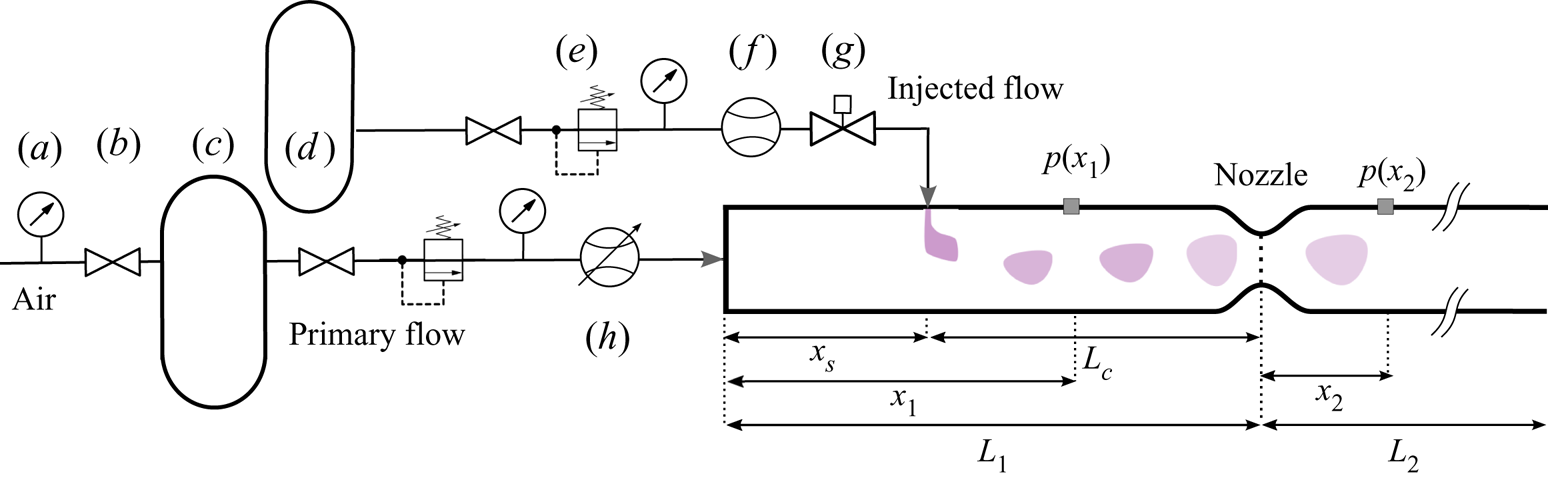
Figure 5. Cambridge Wave Generator with  $(a)$ pressure gauge,
  $(b)$ manual valve,
  $(c)$ air tank,
  $(d)$ secondary gas tank,
  $(e)$ pressure regulator,
  $(\,f)$ mass flow meter,
  $(g)$ fast response solenoid valve and
  $(h)$ mass flow controller.
The nozzles are operated either in subsonic or sonic throat conditions in the test cases considered here ( $\bar {M}_T \leq 1$). It is experimentally verified that the convergent–divergent nozzle has a choking mass flow rate
  $\dot {m} \simeq 10.5\ \textrm {g}\,\textrm {s}^{-1}$, thus the throat reaches sonic conditions with the experimental mass flow rates. The work in De Domenico et al. (Reference De Domenico, Rolland and Hochgreb2019a) showed that these nozzles have a vena contracta factor of
  $\varGamma =0.89$ for the flow conditions considered here. The non-isentropicity parameter
  $\beta$ for each nozzle is determined based on experimental measurements of the pressure drop across the nozzles in § 5.3, following De Domenico et al. (Reference De Domenico, Rolland and Hochgreb2019a). The convergent nozzle, instead, chokes with a mass flow rate of
  $\dot {m} \simeq 13\ \textrm {g}\,\textrm {s}^{-1}$, thus the throat always operates in subsonic conditions for the experimental mass flow rates, with a measured vena contracta factor
  $\varGamma = 0.9381$. A larger vena contracta factor implies a larger effective throat area, which is reflected into a higher choking mass flow rate, as more flow is needed to reach sonic conditions. The minimum effective area experienced by the flow in the convergent-only nozzle is larger as the flow separates as soon as it leaves the throat, while, for the convergent–divergent nozzle, the effective smaller area occurs further downstream, and the flow rearranges itself with a smaller effective throat area.
Pressure measurements are carried out using Kulite XTE-190M piezoresistive pressure transducers, which are flush mounted at locations  $x_1=0.9\ \textrm {m}$ and
  $x_2=1.1\ \textrm {m}$ upstream and downstream of the nozzle. Pressure transducers provide an accuracy of
  $4.0\times 10^{-6}$ full scale (3.5 bar), which translates to
  $1$ Pa for perturbations of 300 Pa. The absolute pressure is logged with a Kulite XTL-190SM transducer (accuracy
  $3.0\times10^{-5}$ full scale), also mounted at
  $x_1$. The pressure transducer signals are acquired using a National Instruments PXIe-4480 module. The signals are sampled at 10 000 Hz and phase-averaged over 100 pulses with a 0.25 Hz repetition rate. Frequencies around 50 Hz (power frequency) and above 400 Hz are filtered out, in accordance with the low frequency range of the excitation.
4.2. Pulse injection
Flow perturbations are generated by pulse injecting a secondary stream of gas into the primary air flow. Since the injected gases (helium, argon, methane or carbon dioxide) have a different entropy and composition than air, the injection generates direct noise, as well as a compositional and entropic disturbance. The injection location is varied to modify the convective length  $L_c$. The convective time delay
  $\tau _c=L_c/\bar {u}_1$ is the time taken for the gas disturbances to convect from the injection location to the nozzle. A fast-response micro-solenoid valve (ASCO Numatics HSM2L7H50V) is connected to the duct via a 0.1 m length of flexible tubing with a 2 mm inner diameter to inject the secondary gas, which enters the duct radially. The valve is actuated using a computer-generated pulse signal, which drives a 24 V power supply. Each pulse lasts
  $\tau _p=100\ \textrm {ms}$. The injector nozzle consists of a Swagelok 1/4” fitting, through which the injected gas enters the tube. The injector can be mounted via one of several ports located along the duct, allowing for different source locations relatively to the nozzle, and thus resulting in a range of convective lengths and times. The ports are aligned with the duct centreline, so that the injected gas enters the duct in the radial direction. Simulations from Rodrigues, Busseti & Hochgreb (Reference Rodrigues, Busseti and Hochgreb2020) and experiments from De Domenico et al. (Reference De Domenico, Shah, Lowe, Fan, Ewart, Williams and Hochgreb2019b) show that the injected plume mixes sufficiently very close to the injection location, allowing for a quasi-one-dimensional approximation. Following the analysis of Broadwell & Breidenthal (Reference Broadwell and Breidenthal1984), it can be demonstrated that the full mixing penetration occurs before the spot enters the nozzle. Corresponding vorticity waves due to the momentum of the injection are shown to be negligible as the spot is convected uniformly with the mean flow. As shown in Howe (Reference Howe2010) and Dowling & Mahmoudi (Reference Dowling and Mahmoudi2015), vorticity noise is negligible for low Mach number flows. The mass flow rate of injected gas (
 $\dot {m}_{He}$,
  $\dot {m}_{Ar}$,
  $\dot {m}_{CH_4}$ or
  $\dot {m}_{CO_2}$) is adjusted using a pressure regulator upstream of the micro-solenoid valve, and monitored with an Alicat M100 mass flow meter (accuracy:
  ${\pm }1\,\%$). The amount of gas is chosen to achieve a given mass fraction for each gas (
 $Y_{He}=0.02$,
  $Y_{CH_4}=0.1$,
  $Y_{Ar}=Y_{CO_2}=0.2$).
4.3. Test cases
The experimental cases examined are chosen in order to demonstrate the influence of nozzle non-isentropicity and compositional effects on the indirect noise generated by perturbations of helium, argon, methane and carbon dioxide. Experiments are carried out with the convergent nozzle (configuration C), or the convergent–divergent nozzle (configuration CD). For each of these, we carry out tests at eleven different air mass flow rates  $\dot {m}$: C1–C11 for the convergent nozzle, and CD1–CD11 for the convergent–divergent nozzle. The experimental cases are shown in tables 1 and 2.
Table 1. Experimental conditions for configuration C (convergent nozzle): upstream mean pressure  $\bar {p}_1$, upstream Mach number
  $\bar {M}_1$, throat Mach number
  $\bar {M}_t$, downstream Mach number
  $\bar {M}_2$, primary mass flow rate
  $\dot {m}$ and injected mass flow rates
  $\dot {m}_{He}$,
  $\dot {m}_{Ar}$,
  $\dot {m}_{CH_4}$ or
  $\dot {m}_{CO_2}$.

Table 2. Experimental conditions for configuration CD (convergent–divergent nozzle): upstream mean pressure  $\bar {p}_1$, upstream Mach number
  $\bar {M}_1$, throat Mach number
  $\bar {M}_t$, downstream Mach number
  $\bar {M}_2$, primary mass flow rate
  $\dot {m}$ and injected mass flow rates
  $\dot {m}_{He}$,
  $\dot {m}_{Ar}$,
  $\dot {m}_{CH_4}$ or
  $\dot {m}_{CO_2}$.

For each experimental condition, we perform eight tests. The secondary gases are injected into the duct with a flow rate  $\dot {m}_{He}$,
  $\dot {m}_{Ar}$,
  $\dot {m}_{CH_4}$ or
  $\dot {m}_{CO_2}$. Tests are carried out for both a ‘long’ and ‘short’ convective length
  $L_c$. For the ‘long’ convective length
  $L_c=0.65\ \textrm {m}$, wave dispersion effects can be identified in the plume (Rodrigues et al. Reference Rodrigues, Busseti and Hochgreb2020), as there is a relatively long convective time delay
  $\tau _c =L_c / \bar {u}_1$ between the generation of direct and indirect noise. For the ‘short’ convective length
  $L_c=0.05$, dispersion and dissipation is minimised and direct and indirect noise occur nearly simultaneously. The results corresponding to the ‘long’ and ‘short’ convective lengths can be compared to identify the indirect noise contribution and minimise the effect of dispersion, as shown in § 3.2. In the experiments, whereas direct noise is evaluated in the ‘long’ tube case, indirect noise is evaluated in the ‘short’ tube case, to minimise the effects of dispersion on the injected mass. In summary, 176 tests are performed in total, which are defined by the experimental condition, the injected gas and the convective length
  $L_c$. For example, ‘test C1–He–long’ refers to the test carried out with a convergent nozzle (in the experimental conditions corresponding to C1 in table 1), where the injected gas is helium and the convective length is long (
 $L_c=0.65\ \textrm {m}$). Each test is repeated for 100 pulses and the resulting pressure measurements are phase-averaged and filtered.
5. Results
In this section, the analytical models derived in §§ 2.2 and 3 are compared with the experimental data acquired in the Entropy Generator Rig. While the experimental points are acquired both in subsonic and transonic conditions, the analytical transfer functions are developed only for subsonic-to-sonic nozzle flows. The non-isentropic behaviour of a supersonic divergent nozzle with losses and a shock is beyond the scope of this work.
5.1. Measurements in the long tube configuration
In the ‘long’ configuration, the convective time delay  $\tau _c$ is longer than the pulse duration
  $\tau _p=100$ ms. As a result, direct and indirect noise are not generated simultaneously. Direct noise is generated during the gas injection (
 $0<t<\tau _p$) and indirect noise is generated as the gas disturbance is accelerated/decelerated through the nozzle (
 $t>\tau _c$).
5.1.1. Upstream of the nozzle
The experimental pressure measurements upstream of the nozzle  ${p'}(x_1)$ for cases C8–He–long and C8–CO2–long are shown in figures 6(a) and 6(b) respectively. In both cases, the acoustic pressure rises sharply during the valve pulse signal (
 $0<t<\tau _p$). This can be explained as follows: during the injection, acoustic waves are generated and reflected back at the inlet and the outlet of the duct with an overall round trip time (time taken for a sound wave to back and forth in the duct)
  $\tau = 2L/\bar{c} \simeq 10\ \textrm {ms}$. This means that sound waves reflect approximately
  $2\tau _p/\tau \approx 20$ times between the inlet and the nozzle before the end of injection time (at
  $t=\tau _p$). As such, the pressure signal corresponds to a superposition of travelling acoustic pulses which accumulate as a pressure signal, each with a small time delay. After the end of the gas injection (at
  $t=\tau _p$) and before the plume of injected gas reaches the nozzle (at
  $t=\tau _c \approx 163$ ms), no acoustic waves are generated in the system. In this case the reverberation model predicts that the pressure should decay exponentially as
 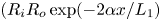 $(R_i R_o \exp(-2\alpha x/L_1)$, as acoustic energy is lost (Rolland et al. Reference Rolland, De Domenico and Hochgreb2017, Reference Rolland, De Domenico and Hochgreb2018). A separate experiment by Rolland et al. (Reference Rolland, De Domenico and Hochgreb2017) determined the attenuation coefficient as a function of the mass flow rate,
  $\alpha \approx 0.47 \bar {M}_1$, where
  $\bar {M}_1$ is the upstream Mach number. Since
  $R_i$,
  $\alpha$,
  $\tau$ and
  $L_1$ are known, the decay rate in the experimental signal for
  $\tau _p < t < \tau _c$ can be directly related to the amplitude of the nozzle reflection coefficient
  $R_o$. The modelled exponential decay corresponding to the experimentally determined value of
  $R_o$ is shown with a dashed line in figure 6. Once the secondary gas perturbation reaches the nozzle (at
  $t=\tau _c$ in figure 6), indirect noise is generated. This can be seen in the experimental data: the pressure measurements deviate from the exponential decay curve at
  $t \approx \tau _c$ for both C8–He–long and C8–CO2–long. For C8–He–long, the indirect noise is negative, while for C8–CO2–long it is positive. This is consistent with the relative higher excess densities of helium with respect to air and lower excess density of carbon dioxide with respect to air. The source identification technique outlined in § 3.2 can be applied to identify the contributions of the direct and indirect acoustic sources
  ${\rm \pi} _d^+$ and
  ${\rm \pi} _i^-$ to the measured acoustic pressure. The resulting source signals
  ${{\rm \pi} }_1$ (from which the effects of the multiple reflections have been removed) for cases C8–He–long and C8–CO2–long are shown in figure 7.

Figure 6. Experimental pressure fluctuation upstream of the nozzle  $p'/\bar{\gamma} \bar {p}(x_1,t)$ (black solid line) for
  $(a)$ case C8–He–long and
  $(b)$ C8–CO2–long. Valve pulse duration
  $\tau _p$ (black dashed line), convective time delay
  $\tau _c$ (light grey dashed line), and exponential decay fit of the acoustic energy loss (red dashed line).
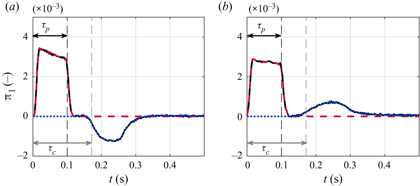
Figure 7. Upstream acoustic source  ${\rm \pi} _1$ as a function of time (black solid line) for
  $(a)$ case C8–He–long and
  $(b)$ C8–CO2–long. Direct noise contribution
  $(1+R_o)(1+R_i){\rm \pi} _d^+$ (red dashed line) and indirect noise contribution
  $(1+R_i){\rm \pi} _i^-$ (blue dotted line). Valve pulse duration
  $\tau _p$ (black dashed line), convective time delay
  $\tau _c$ (light grey dashed line).
For both cases the acoustic source signal  ${\rm \pi} _1$ is a succession of two acoustic pulses. The first pulse coincides with the valve pulse signal (from
  $t=0$ to
  $t=\tau _p$) and corresponds to the direct noise
  ${\rm \pi} _d^+$ generated during the injection. The second pulse appears at a time delay consistent with the convective time
  $\tau _c$ and is the backward-propagating indirect noise source
  ${\rm \pi} _i^-$. For case C8–He–long the indirect noise source is negative, while for C8–CO2–long it is positive. The indirect noise source signal
  ${\rm \pi} _i^-$ is spread out, indicating that the helium and carbon dioxide perturbations have undergone dispersion over the convective length
  $L_c=0.65\ \textrm {m}$.
5.1.2. Downstream of the nozzle
The experimental pressure measurements downstream of the nozzle  ${p'}(x_2)$ for cases C8–He–long and C8–CO2–long are shown in figure 8. The signal is truncated at
  $t \approx 2 L_2/\bar {c}_2 \approx 350$ ms, the time after which the outlet of the system can no longer be considered to be anechoic. The acoustic model in § 3.1 indicates that the signal downstream of the nozzle is a combination of (i) direct and indirect noise generated upstream of the nozzle and transmitted downstream, as well as (ii) indirect noise generated downstream of the nozzle. For
  $t<\tau _c$, the compositional and entropic perturbation has not yet reached the nozzle, and only direct noise is generated in the system. In this case, our model predicts that the ratio of the acoustic pressures upstream and downstream of the nozzle is approximately
  $T_o/(1+R_o)$, as shown in (3.11). Since
  $R_o$ is known, we can take advantage of this to obtain a value for
  $T_o$. We can then use source identification to identify the two contributions to the acoustic pressure: the transmitted upstream pressure
  $\mathcal {F} {\rm \pi}_2$ and the forward-propagating indirect noise generated at the nozzle
  ${\rm \pi} _i^+$. These are shown in figure 8. The forward-propagating indirect noise contribution
  ${\rm \pi} _i^+$ appears in the acoustic pressure signal at
  $t\approx \tau _c$ as expected. The contribution is opposite in sign to that of the backward-propagating indirect noise
  ${\rm \pi} _i^-$ shown in figure 7 (positive for helium, negative for carbon dioxide).

Figure 8. Experimental pressure fluctuations downstream of the nozzle  $p'/(\bar{\gamma} \bar {p}(x_2,t))$ (black solid line) for
  $(a)$ case C8–He–long and
  $(b)$ C8–CO2–long. Transmitted upstream source
  $\mathcal {F} {\rm \pi}_2$ (red dashed line) and forward-propagating indirect noise source
  ${\rm \pi} _i^+$ (blue dotted line). Valve pulse duration
  $\tau _p$ (black dashed line), convective time delay
  $\tau _c$ (light grey dashed line).
5.2. Short tube configuration
In the ‘short’ configuration, the convective time delay  $\tau _c \simeq 0.001\text {--}0.01\ \textrm {s}$ is shorter than the pulse duration
  $\tau _p=100\ \textrm {ms}$. The short convection time minimises the effects of dissipation and dispersion on the composition spots and, as a result, we expect that direct and indirect noise are generated simultaneously (for
  $\tau _c<t<\tau _p$), and that no noise is generated once the gas perturbation has fully convected through the nozzle (for
  $t>\tau _c+\tau _p$).
5.2.1. Upstream of the nozzle
The experimental pressure measurements upstream of the nozzle  ${p'}(x_1)$ for cases C8–He–short and C8–CO2–short are shown in figure 9. As with cases C8–He–long and C8–CO2–long shown in figure 6, the acoustic pressure rises sharply during the valve pulse signal (for
  $0<t<\tau _p=100\ \textrm {ms}$). Notably, the maximum pressure fluctuation reached at
  $t \approx \tau _p$ for C8–He–short is much lower than in C8–He–long. Conversely, the maximum pressure reached for C8–CO2–short is much higher than for C8–CO2–long. This is because in the ‘short’ cases, direct and indirect are generated simultaneously, while in the ‘long’ cases only direct noise is generated for
  $t<\tau _p$. Since the indirect noise generated by a helium disturbance leads to a negative pressure fluctuation upstream of the nozzle (as shown in figure 6a), the direct noise and indirect noise interact deconstructively for C8–He–short, and the maximum pressure is lower than of the direct noise alone measured for C8–He–long. Conversely, the indirect noise generated by a carbon dioxide disturbance leads to a positive pressure fluctuation upstream of the nozzle, which results in a larger overall pressure fluctuation for C8–CO2–short than for C8–CO2–long.
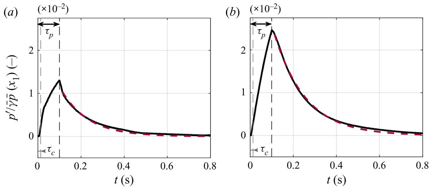
Figure 9. Experimental pressure fluctuations upstream of the nozzle  $p'/(\bar{\gamma} \bar {p}(x_1,t))$ (black solid line) for
  $(a)$ case C8–He–short and
  $(b)$ C8–CO2–short. Valve pulse duration
  $\tau _p$ (black dashed line), convective time delay
  $\tau _c$ (light grey dashed line) and exponential decay fit (red dashed line).
Once the compositional and entropic disturbance has fully convected through the nozzle (at  $t \approx \tau _c +\tau _p$), no noise is generated in the system. As such, we expect the acoustic pressure to decay exponentially as described in (3.10). The theoretical exponential decay is in good agreement with the experimental measurements as shown in figure 9. We can apply the source identification method to extract the acoustic source waves in the system in cases C8–He–short and C8–CO2–short, as shown in figure 10. The acoustic source signal
  ${\rm \pi} _1$ corresponds to the superposition of direct and indirect noise sources
  ${\rm \pi} _d^+$ and
  ${\rm \pi} _i^-$. Since the convective time delay
  $\tau _c$ is very short, these sources are almost merged. As a result, the overall acoustic source appears as a single acoustic pulse. The difference between the ‘short’ and ‘long’ cases is the convective length
  $L_c$, which affects the time at which the indirect noise is generated, while the direct noise source
  ${\rm \pi} _d^+$ is the same in both cases. In the ‘long’ tube configuration, the direct noise source
  ${\rm \pi} _d^+$ can be isolated, as shown in figure 7, and then subtracted from the overall acoustic source
  ${\rm \pi} _1$ for the ‘short’ cases shown in figure 10. This leaves us with the indirect acoustic source
  ${\rm \pi} _i^-$, which is shown in figure 10. The shape of this recovered indirect noise source shows that much less diffusion/dispersion has occurred than in the corresponding ‘long’ cases. This enables us to compare the results to the predictions of the theoretical models in § 2, which do not account for dispersion and diffusion.

Figure 10. Upstream acoustic source  ${\rm \pi} _1$ as a function of time (black solid line) for
  $(a)$ case C8–He–short and
  $(b)$ C8–CO2–short. Valve pulse duration
  $\tau _p$ (black dashed line), convective time delay
  $\tau _c$ (light grey dashed line). Direct noise contribution
  $(1+R_o)(1+R_i){\rm \pi} _d^+$ (red dashed line) and indirect noise contribution indirect noise contribution
  $(1+R_i){\rm \pi} _i^-$ (blue dotted line).
5.3. Comparison of the experimental data with the non-isentropic nozzle models
The experimental results shown in §§ 5.1 and 5.2 enable us to recover measurements of the nozzle reflection and transmission coefficients  $R_o$ and
  $T_o$ as well as the forward- and backward-propagating indirect noise waves
  ${\rm \pi} _i^+$ and
  ${\rm \pi} _i^-$. These measurements can be compared to the non-isentropic nozzle model derived in § 2.2 and appendix A. The non-isentropic nozzle model requires as inputs the values of the chemical potential function
  $\varPsi$ throughout the nozzle, the heat-capacity factor
  $\aleph$ as well as the non-isentropicity parameter
  $\beta =A_j/A_2$. The flow noise, which is uncorrelated with the low-frequency pulse, is removed by cycle averaging the pulse sequence, which acts as a low-frequency filter. In this way, transmitted sound waves generated by the injection can be isolated. From the measured averaged peak values of the direct and indirect noise upstream and downstream of the nozzle, we obtain the experimental values of the reflection and transmission coefficients. The measurements downstream of the nozzle display a lower signal-to-noise ratio and higher background noise level than the measurements upstream, so the transmission coefficients are less accurate than the reflection coefficients. This suggests that measuring the acoustic properties upstream of the nozzle constitute a more accurate way to determine the transfer functions of the nozzle, as multiple reflections enhance the signal, obtaining a standard deviation on the reflection coefficient of
  $10\text{--}12\,\%$, lower than the standard deviation on the transmission coefficient obtained from the measurements downstream of
  $15\text{--}17\,\%$.
5.3.1. Evaluation of entropy and composition waves
The chemical potential function  $\varPsi$ and the heat-capacity factor
  $\aleph$ are needed to determine the amplitude of the entropy and composition waves and the nozzle transfer functions (Magri Reference Magri2017). These are calculated using thermo-chemical data obtained from Lemmon, McLinden & Friend (Reference Lemmon, McLinden and Friend1998) as
 \begin{gather} \varPsi = \frac{1}{\bar{c}_p\bar{T}} \sum_{n=1}^{N} \left(\frac{\mu_i}{W_i} \right) \frac{\textrm{d}Y_i}{\textrm{d}Z} = \frac{ (h_{inj} - T s_{inj} ) - (h_{air} - T s_{air}) }{{h}_{air}} \nonumber\\ = \frac{h_{inj}- h_{air}}{{h}_{air}} - \frac{T (s_{inj}-s_{air})}{{h}_{air}}, \end{gather}
 \begin{gather}\aleph = \frac{R'}{\bar{R}} - \frac{c_p'}{\bar{c}_p} = \dfrac{W_{air} - W_{inj}}{W_{inj} } - \frac{c_{p,inj} - c_{p,air}}{c_{p,air} }, \end{gather}
where  $()_{air}$ and
  $()_{inj}$ are the mean flow of air and the injected gas, respectively. We can now evaluate (2.10) in the context of a generic synthetic wave generator with the pulse injection of a secondary gas. We define
  $\varphi '_e$ and
  $\varphi '_m$ as
 \begin{equation} \varphi'_e = \frac{h_{tot}'}{\bar{h}} \simeq \frac{\dot{m}_{inj}}{\dot{m}_{air}}\frac{h_{inj}}{h_{air}} = Y_{inj}\frac{h_{inj}}{h_{air}} , \quad \varphi'_m = \xi = \frac{\dot{m}_{inj}}{\dot{m}_{air}} = Y_{inj}. \end{equation}
 Considering a low Mach number mean flow ( $\bar{M}\ll 1$), the higher-order terms multiplied by
  $\bar{M}^2$ in (2.10) can be neglected, so that the entropy wave
  $\sigma$ can be computed as
 \begin{equation} \sigma \simeq Y_{inj}\frac{T (s_{inj} - s_{air})}{h_{air}} = Y_{inj}\frac{ s_{inj} - s_{air}}{c_{p,air}}. \end{equation}
The indirect noise waves generated by the nozzle are  ${\rm \pi} _i^{\pm } = {\rm \pi}_{\xi }^{\pm } + {\rm \pi}_{\sigma }^{\pm }$. To obtain these, the amplitude of the impinging entropic and compositional waves
  $\sigma$ and
  $\xi$ are evaluated using the wave generation model in § 2 and (5.4). The overall indirect noise can then be calculated using the non-isentropic nozzle transfer functions as
  ${{{\rm \pi} _i^{\pm }}= ({{\rm \pi} _{\xi }^{\pm }}/{\xi }) {\xi } + ({{\rm \pi} _{\sigma }^{\pm }}/{\sigma }) {\sigma }}$.
5.3.2. Determination of the non-isentropicity parameter  $\beta$

The non-isentropicity parameter  $\beta$ accounts for the pressure losses occurring in the system, and, following the procedure described in De Domenico et al. (Reference De Domenico, Rolland and Hochgreb2019a), can be obtained from the experimental measurements of the mean pressure upstream and downstream of the nozzle
  $\bar {p}_1$ and
  $\bar {p}_2$ (De Domenico et al. Reference De Domenico, Rolland and Hochgreb2019a). For a particular mass flow rate
  $\dot {m}$, each value of
  $\beta$ corresponds to a particular pressure
  $\bar {p}_1$ (figure 11), hence, to a specific rate of mean pressure loss. Therefore, the accuracy in
  $\beta$ reflects the accuracy in the measurements of the mass flow rate and the corresponding mean pressure loss measurements. As shown in De Domenico et al. (Reference De Domenico, Rolland and Hochgreb2019a), for the convergent–divergent nozzle, the amount of pressure losses, and consequently the non-isentropicity parameter
  $\beta$ are a function of the mass flow rate
  $\dot {m}$. Using a least-squares fit to the measured pressure drop and mean mass flow rate, we obtain
 \begin{equation} \beta_{CD}=f(\dot{m})= 23305.57 \dot{m}^3 -538.21 \dot{m}^2 + 2.48 \dot{m} + 0.03, \end{equation}
which is an accurate approximation for the convergent–divergent nozzle (figure 11), where  $\dot {m}$ is the mass flow rate in
  $\textrm {kg}\,\textrm {s}^{-1}$. The values of
  $\beta _{CD}$ range from 0.022 to 0.032. From the experimental data, the convergent-only nozzle behaves as an orifice plate with
  $\varGamma = 0.9381$. As the flow exits the nozzle as a jet, the area
  $A_j$ nearly corresponds to the throat area and it is experimentally determined that
  $\beta _c \simeq 1.03$ for all the mass flow rates (
 $A_j \simeq 1.03 \varGamma A_T$). The present experiment shows that it is possible to account for the non-isentropicity of the discharge in nozzle guide vanes, which typically operate under choking conditions, using simple models.

Figure 11. Upstream pressure  ${p}_1$ as a function of the mass flow rate
  $\dot {m}$. Experimental measurements for the convergent nozzle C (red filled circles) and the convergent–divergent nozzle CD (blue open circles), analytical predictions for the convergent nozzle with
  $\beta _C$ (red solid line), convergent–divergent nozzle with
  $\beta _{CD}$ (blue dashed line), orifice plate limit for
  $\beta = A_t/A_2$ (black dotted line) and fully isentropic nozzle for
  $\beta = 1$ (black dash-dot line).
5.4. Determination of the acoustic reflection and transmission coefficients
The acoustic reflection and transmission coefficients  $R_o$ and
  $T_o$ extracted from the experimental data for the convergent and convergent–divergent nozzle are shown in figure 12. These measurements are compared to three implementations of the non-isentropic nozzle model: (i) the convergent nozzle for
  $\beta =\beta _C$ (solid lines), (ii) the convergent–divergent nozzle with
  $\beta =\beta _{CD}$ (dashed lines) and (iii) the orifice plate limit case (dotted black lines). The fully isentropic limit case for
  $\beta =1$, which is commonly used in the literature, is shown in dash-dotted black lines. The reflection and transmission coefficients are plotted as a function of the throat Mach number
  $\bar{M}_T$. As shown in De Domenico et al. (Reference De Domenico, Rolland and Hochgreb2019a), the isentropic model (Marble & Candel Reference Marble and Candel1977; Magri et al. Reference Magri, O'Brien and Ihme2016) shows a discontinuity for
  $M_T=1$, and the coefficients for choked conditions are plotted with square black markers. As the mass flow rate increases, the experimental data show that the transmission coefficient
  $T_o$ decreases and the reflection coefficient
  $R_o$ increases. This trend is correctly recovered by the convergent and convergent–divergent nozzle models. These models predict that the convergent–divergent nozzle has a higher transmission coefficient and a lower reflection coefficient than the convergent nozzle, which is verified by the experimental results.

Figure 12.  $(a)$ Acoustic reflection coefficient
  $R_{o1} = {\rm \pi}_1^- / {\rm \pi}_1^+$ and
  $(b)$ acoustic transmission coefficient
  $T_{o1} ={\rm \pi} _2^+ / {\rm \pi}_1^+$ as a function of the throat Mach number
  $M_T$. Convergent nozzle: theory (red solid lines), experimental measurement (red filled circles). Convergent–divergent nozzle: theory (blue dashed lines), experimental measurement (blue open circles). Fully isentropic nozzle (black dash-dot line), orifice plate model (black dotted line).
The isentropic nozzle model predicts zero reflection and full transmission in the subsonic range (since  $A_1=A_2$ and the nozzle is acoustically compact). The assumption of isentropicity is inadequate, as explained by De Domenico et al. (Reference De Domenico, Rolland and Hochgreb2019a). Conversely, the limit case of a fully non-isentropic divergent jet (orifice plate model where
  $\beta =A_t/A_2$) underestimates
  $T_o$ and overestimates
  $R_o$ for the convergent–divergent nozzle. Instead, as expected, the reflection and transmission coefficients of the convergent nozzle show a similar behaviour to the orifice plate transfer function.
In the sonic regime, all four models predict a nearly identical reflection coefficient  $R_o$, which is in good agreement with the experimental data. This is because all the models assume that the upstream section of the nozzle is fully isentropic. The models also predict similar values of the transmission coefficient
  $T_o$, which are in good agreement with the experimental measurements for both nozzles. An essential difference between the isentropic and non-isentropic models lies in the behaviour of the system as it crosses subsonic to sonic conditions: all isentropic models (Marble & Candel Reference Marble and Candel1977; Magri Reference Magri2017) display a discontinuity in the nozzle transfer functions while crossing from subsonic to sonic (dashed-dotted lines).
5.5. Determination of the indirect and composition noise transfer functions
The amplitude of the indirect noise waves  ${\rm \pi} _i^{\pm } = {\rm \pi}_{\sigma }^{\pm } + {\rm \pi}_{\xi }^{\pm }$ is measured for all the experimental cases, and used to compute the forward and backward indirect noise nozzle transfer functions
  ${\rm \pi} _i^+/\xi _1$ and
  ${\rm \pi} _i^-/\xi _1$. These are compared to the theoretical models of the convergent and convergent–divergent nozzles as well as the limit cases of the isentropic nozzle and orifice plate in figure 13. As previously discussed, the isentropic models are discontinuous at the choking point due to the jump from subsonic flow to sonic flow at
  $\bar{M}_T =1$ (dash-dotted lines). For the most part, the experimental indirect noise measurements lie somewhere in between the isentropic nozzle and orifice plate limit cases, confirming that the convergent and convergent–divergent nozzles tested here are intermediate situations. The theoretical models for the convergent and convergent–divergent nozzle are in relatively good agreement with the experimental results, while the isentropic models are unable to capture the experimental trends at all. This was observed in De Domenico et al. (Reference De Domenico, Rolland and Hochgreb2019a) for the upstream-propagating entropy noise. The present work generalises these results to multi-component gases with upstream and downstream-propagating compositional waves. The non-isentropic model predicts that the convergent–divergent nozzle produces slightly less indirect noise than the convergent nozzle. This is verified by the experimental results for helium and methane. Conversely, for argon and carbon dioxide, the opposite appears to be the case.

Figure 13. Forward- and backward-propagating indirect noise transfer functions  ${\rm \pi} _i^+/\xi _1$ and
  ${\rm \pi} _i^-/\xi _1$ as a function of the throat Mach number
  $\bar{M}_T$ for (a,b) CO
 $_2$, (c,d) methane, (e,f) argon, (g,h) helium. Convergent nozzle: theory (solid lines), experiments (filled circles). Convergent–divergent nozzle: theory (dashed lines), experiments (open circles). Fully isentropic nozzle (black dash-dot line), orifice plate model (black dotted line).
We can suggest several hypotheses for these discrepancies and different physical behaviour. The first is the fact is that the convergent–divergent nozzle is substantially longer than the convergent nozzle ( $L_n=0.254\ \textrm {m}$ and
  $L_n=0.024\ \textrm {m}$ respectively). The consequence of this is two-fold. First, this means that the two nozzles correspond to two different Helmholtz numbers
  $\textit{He}= L_n/(\tau _p \bar {c})$ (which represent the nozzle compactness). Indeed, we have
  $He \approx 7.4 \times 10^{-3}$ for the convergent–divergent nozzle and
  ${\textit{He}}\approx 7 \times 10^{-4}$ for the convergent nozzle. In other words, the convergent–divergent nozzle is less compact than the convergent nozzle, and these non-compact effects might affect the result. However, the results in Magri (Reference Magri2017) suggest that for such small values of He, frequency effects should be negligible. The second effect of the nozzle length is related to the dispersion and diffusion of entropic and compositional waves inside the nozzle, which the model does not account for. One might expect these effects to be more pronounced in the convergent–divergent nozzle (because it is longer), and to vary depending on the gas being considered (as shown in De Domenico et al. Reference De Domenico, Rolland and Hochgreb2019a). This may have an effect on the indirect noise generation inside the nozzle, affecting the various gases differently. Additionally, our model assumes that the entropic and compositional waves convected through the nozzle are one-dimensional. In reality, these disturbances are likely to be non-uniformly distributed across the duct cross-section, as demonstrated by recent numerical simulations on the dispersion of synthetic composition spots in a duct (Rodrigues et al. Reference Rodrigues, Busseti and Hochgreb2020). This may affect the amplitude of the indirect noise generated by the nozzle as shown in Zheng et al. (Reference Zheng, Huet, Giauque, Cléro and Ducruix2015), although the effects should be small for the Helmholtz numbers considered here. Finally, part of the discrepancy could be due to (weakly) nonlinear effects. While the mass fraction of helium and methane injected into the main flow is relatively low (
 $Y_{He}=0.02$ and
  $Y_{CH_4}=0.1$ respectively.), the amount of argon and carbon dioxide injected (
 $Y_{Ar}=Y_{CO_2}=0.2$) may be locally large enough to stray from the linear perturbation model employed here.
5.5.1. Indirect noise ratio
Although the ratio of entropic to compositional noise  $|{\rm \pi} _{\sigma }^{\pm }/{\rm \pi} _{\xi }^{\pm }|$ cannot be directly obtained from the experimental data, as they are generated at the same time, we can use the non-isentropic model to estimate it. The analytical model predicts that the noise ratios are
 \begin{equation} \left|\frac{{\rm \pi}_{\sigma}^{\pm}}{{\rm \pi}_{\xi}^{\pm}}\right| = \left\{1.39; 1.24; 1.12; 1.22\right\}\quad\text{for}\ \left\{\text{He}; \text{CH}_4; \text{Ar}; \text{CO}_2\right\}. \end{equation}
Based on this, the gases considered in these experiments generate comparable amounts of entropic and compositional indirect noise, showing that compositional indirect noise has to be included to correctly evaluate the overall indirect noise. Given that the expected gas turbine mixture fraction fluctuations are of the order of  $5\text {--}10\,\%$ (Magri Reference Magri2017; Giusti et al. Reference Giusti, Magri and Zedda2019), which is similar to the experimental mass fractions used in this work, both entropic and compositional fluctuations can lead to indirect noise magnitudes of the same order as direct noise.
6. Conclusion
The generation of indirect noise in non-isentropic nozzles is investigated analytically and experimentally. The one-dimensional analytical framework developed consists of three components: (i) a low-order model to compute the acoustic, compositional and entropic waves generated at a wave generator, (ii) a generalisation of the non-isentropic low-order model developed by De Domenico et al. (Reference De Domenico, Rolland and Hochgreb2019a) to multi-component gases to account for composition-to-sound conversion and (iii) the relationship between the acoustic sources in a reverberating system and the resulting pressure traces. A series of controlled experiments is conducted on the Cambridge Wave Generator to measure the upstream- and downstream-propagating indirect noise generated by the acceleration of helium, methane, argon and carbon dioxide perturbations through two non-isentropic compact nozzles in subsonic and sonic conditions; generalising to more gases and conditions the experiments performed by Rolland et al. (Reference Rolland, De Domenico and Hochgreb2018). The analytical framework is used to perform source identification, whereby the direct and indirect noise generated in the experiment can be extracted and separated. Comparison of the experimental data with the isentropic and non-isentropic models shows that the former is inadequate to capture the behaviour of the acoustic noise over the subsonic-to-sonic range considered and might have detrimental consequences on the accuracy of the predictions for combustion noise. The comparison between experimental data and analytical model shows that the extent of entropic and compositional indirect noise produced in the experiment by the injection of the various gases is similar, which indicates that compositional indirect noise can be as significant as indirect noise generated by temperature inhomogeneities (also known as ‘entropy noise’). Given that the expected gas turbine mixture fraction fluctuations are of the order of 5–10 % (Giusti et al. Reference Giusti, Magri and Zedda2019), which is similar to the experimental mass fractions used in this work, both entropic and compositional fluctuations can lead to indirect noise of the same order of magnitude as direct noise.
From a fundamental point of view, this work reports the first experimental evidence of the importance of considering compositional noise and non-isentropicity of a system in the evaluation of the indirect noise generated. From an application point of view, this work opens up new possibilities for accurate modelling of thermoacoustic oscillations and indirect noise, which is directly relevant to aeronautical gas turbine combustors, in which temperature and compositional fluctuations can be significant.
Acknowledgements
This work was supported by the UK Engineering and Physical Sciences Research Council (EPSRC) grant EP/K02924X/1. F.D.D. is supported by a Junior Research Fellowship by Gonville and Caius College; E.O.R. is supported by an EPSRC/DTA studentship (University of Cambridge); J.R. is supported by a Qualcomm/DTA Studentship. L.M. acknowledges the support from the Royal Academy of Engineering Research Fellowships Scheme.
Declaration of interests
The authors report no conflict of interest.
Appendix A. Solution of the non-isentropic jump conditions
The isentropic and non-isentropic jumps can be linearised and decomposed in terms of wave amplitudes  ${\rm \pi} ^+$,
  ${\rm \pi} ^-$,
  $\sigma$ and
  $\xi$.
A.1. Transfer functions of a wave generator
The jump conditions across the wave generator (2.7) can be expressed in matrix form as
 \begin{equation} \boldsymbol{\mathsf{X}}_{2} \boldsymbol{w}_2 - \boldsymbol{\mathsf{X}}_{1} \boldsymbol{w}_1 = \boldsymbol{\varPhi}, \end{equation}
where  $\boldsymbol{\mathsf{X}}$ is the matrix
 \begin{align} {{
\begin{bmatrix} 1 + \dfrac{1}{\bar{M}} & 1 -
\dfrac{1}{\bar{M}} & -1 & - (\varPsi +\aleph)
\\ \left( 1 + \dfrac{1}{\bar{M}}
\right)^2 & \left( 1 - \dfrac{1}{\bar{M}} \right)^2 & -1 &
- (\varPsi + \aleph) \\ 1 +
\dfrac{1}{\bar{M}} +\dfrac{ (\bar{\gamma} -1 )(1 +
\bar{M})}{1+\dfrac{\bar{\gamma}-1}{2}\bar{M}^2} & 1 -
\dfrac{1}{\bar{M}} + \dfrac{ (\bar{\gamma} -1
)(1-\bar{M})}{1+\dfrac{\bar{\gamma}-1}{2}\bar{M}^2} &
\dfrac{1}{1+\dfrac{\bar{\gamma}-1}{2}\bar{M}^2} -1 &
-(\varPsi+\aleph) +
\dfrac{\varPsi}{1+\dfrac{\bar{\gamma}-1}{2}\bar{M}^2}
\\ 0 & 0 & 0 & 1
\end{bmatrix},}} \end{align}
\begin{align} {{
\begin{bmatrix} 1 + \dfrac{1}{\bar{M}} & 1 -
\dfrac{1}{\bar{M}} & -1 & - (\varPsi +\aleph)
\\ \left( 1 + \dfrac{1}{\bar{M}}
\right)^2 & \left( 1 - \dfrac{1}{\bar{M}} \right)^2 & -1 &
- (\varPsi + \aleph) \\ 1 +
\dfrac{1}{\bar{M}} +\dfrac{ (\bar{\gamma} -1 )(1 +
\bar{M})}{1+\dfrac{\bar{\gamma}-1}{2}\bar{M}^2} & 1 -
\dfrac{1}{\bar{M}} + \dfrac{ (\bar{\gamma} -1
)(1-\bar{M})}{1+\dfrac{\bar{\gamma}-1}{2}\bar{M}^2} &
\dfrac{1}{1+\dfrac{\bar{\gamma}-1}{2}\bar{M}^2} -1 &
-(\varPsi+\aleph) +
\dfrac{\varPsi}{1+\dfrac{\bar{\gamma}-1}{2}\bar{M}^2}
\\ 0 & 0 & 0 & 1
\end{bmatrix},}} \end{align}
 $\boldsymbol {w}$ is the vector of the wave amplitudes
 \begin{equation} \boldsymbol{w} = \begin{bmatrix} {\rm \pi}^+, {\rm \pi}^- , \sigma, \xi \end{bmatrix}^{T}, \end{equation}
and  $\boldsymbol {\varPhi }$ is the vector of the source terms
 \begin{equation} \boldsymbol{\varPhi} = \begin{bmatrix} \varphi_{\dot{m}}, \varphi_{M} , \varphi_{e}, \varphi_{\xi} \end{bmatrix}^{T}. \end{equation}
A.2. Jump conditions across a non-isentropic nozzle
The jump conditions across a non-isentropic subsonic nozzle modelled as described in § 2.2 in (2.11), (2.13)), can be expressed in matrix form as
 \begin{equation} \left. \begin{gathered} \boldsymbol{\mathsf{X}}_{1} \boldsymbol{w}_1 = \boldsymbol{\mathsf{X}}_{j} \boldsymbol{w}_j, \\ \boldsymbol{\mathsf{Y}}_{j} \boldsymbol{w}_j = \boldsymbol{\mathsf{Y}}_{2} \boldsymbol{w}_2, \end{gathered} \right\} \end{equation}
where  $\boldsymbol{\mathsf{X}}$ and
  $\boldsymbol{\mathsf{Y}}$ are transfer matrices
 \begin{equation} \boldsymbol{\mathsf{X}} =
\begin{bmatrix} 1 + \dfrac{1}{\bar{M}} & 1 -
\dfrac{1}{\bar{M}} & -1 & -\varPsi - \aleph
\\ \dfrac{(\bar{\gamma} - 1)\left( 1 +
{\bar{M}} \right) }{1+\displaystyle \frac{\bar{\gamma} -1}{2}\bar{M}^2} &
\dfrac{(\bar{\gamma} - 1)\left( 1 - {\bar{M}} \right)
}{1+\displaystyle \frac{\bar{\gamma} -1}{2}\bar{M}^2} &
\dfrac{1}{1+\displaystyle \frac{\bar{\gamma} -1}{2}\bar{M}^2} & \dfrac{\varPsi
}{1+\displaystyle \frac{\bar{\gamma} -1}{2}\bar{M}^2} \\ 0 &
0 & 1 & 0 \\ 0 & 0 & 0 & 1
\end{bmatrix}, \end{equation}
\begin{equation} \boldsymbol{\mathsf{X}} =
\begin{bmatrix} 1 + \dfrac{1}{\bar{M}} & 1 -
\dfrac{1}{\bar{M}} & -1 & -\varPsi - \aleph
\\ \dfrac{(\bar{\gamma} - 1)\left( 1 +
{\bar{M}} \right) }{1+\displaystyle \frac{\bar{\gamma} -1}{2}\bar{M}^2} &
\dfrac{(\bar{\gamma} - 1)\left( 1 - {\bar{M}} \right)
}{1+\displaystyle \frac{\bar{\gamma} -1}{2}\bar{M}^2} &
\dfrac{1}{1+\displaystyle \frac{\bar{\gamma} -1}{2}\bar{M}^2} & \dfrac{\varPsi
}{1+\displaystyle \frac{\bar{\gamma} -1}{2}\bar{M}^2} \\ 0 &
0 & 1 & 0 \\ 0 & 0 & 0 & 1
\end{bmatrix}, \end{equation}
 \begin{align} \boldsymbol{\mathsf{Y}} =
\begin{bmatrix} 1 + \dfrac{1}{\bar{M}} & 1 -
\dfrac{1}{\bar{M}} & -1 & -\varPsi -
\aleph\\ \dfrac{(\bar{\gamma} - 1)\left( 1 +
{\bar{M}} \right) }{1+\dfrac{\bar{\gamma} -1}{2}\bar{M}^2} &
\dfrac{(\bar{\gamma} - 1)\left( 1 - {\bar{M}} \right)
}{1+\dfrac{\bar{\gamma} -1}{2}\bar{M}^2} &
\dfrac{1}{1+\dfrac{\bar{\gamma} -1}{2}\bar{M}^2} &
\dfrac{\varPsi}{1+\dfrac{\bar{\gamma} -1}{2}\bar{M}^2}
\\ \bar{c} \left( \dfrac{A_2}{A}
\dfrac{1}{ \bar{M} } + 2 + \bar{M} \right) & \bar{c} \left(
\dfrac{A_2}{A} \dfrac{1}{ \bar{M} } - 2 + \bar{M} \right) &
-\bar{M} \bar{c} & - (\varPsi + \aleph) \bar{M} \bar{c}
\\ 0 & 0 & 0 & 1
\end{bmatrix}. \end{align}
\begin{align} \boldsymbol{\mathsf{Y}} =
\begin{bmatrix} 1 + \dfrac{1}{\bar{M}} & 1 -
\dfrac{1}{\bar{M}} & -1 & -\varPsi -
\aleph\\ \dfrac{(\bar{\gamma} - 1)\left( 1 +
{\bar{M}} \right) }{1+\dfrac{\bar{\gamma} -1}{2}\bar{M}^2} &
\dfrac{(\bar{\gamma} - 1)\left( 1 - {\bar{M}} \right)
}{1+\dfrac{\bar{\gamma} -1}{2}\bar{M}^2} &
\dfrac{1}{1+\dfrac{\bar{\gamma} -1}{2}\bar{M}^2} &
\dfrac{\varPsi}{1+\dfrac{\bar{\gamma} -1}{2}\bar{M}^2}
\\ \bar{c} \left( \dfrac{A_2}{A}
\dfrac{1}{ \bar{M} } + 2 + \bar{M} \right) & \bar{c} \left(
\dfrac{A_2}{A} \dfrac{1}{ \bar{M} } - 2 + \bar{M} \right) &
-\bar{M} \bar{c} & - (\varPsi + \aleph) \bar{M} \bar{c}
\\ 0 & 0 & 0 & 1
\end{bmatrix}. \end{align}
To obtain a relationship between the waves at the inlet and outlet of the nozzle  $\boldsymbol {w}_1$ and
  $\boldsymbol {w}_2$, we can write
 \begin{equation} \boldsymbol{\mathsf{X}}_{1} \boldsymbol{w}_1 = \boldsymbol{\mathsf{X}}_{j} \boldsymbol{\mathsf{Y}}_{j}^{-1} \boldsymbol{\mathsf{Y}}_{2} \boldsymbol{w}_2, \end{equation}
or in terms of ingoing and outgoing waves  $\boldsymbol {w}_i=[{\rm \pi} ^+_1, {\rm \pi}^-_2, \sigma _1, \xi _1]^T$ and
  $\boldsymbol {w}_o=[{\rm \pi} ^+_2, {\rm \pi}^-_1, \sigma _2, \xi _2]^T$
 \begin{equation} \boldsymbol{\mathsf{X}}_{i} \boldsymbol{w}_i = \boldsymbol{\mathsf{X}}_{o} \boldsymbol{w}_o, \end{equation}
where  $\boldsymbol{\mathsf{X}}_{i}$ and
  $\boldsymbol{\mathsf{X}}_{o}$ are permutations of
  $\boldsymbol{\mathsf{X}}_{1}$ and
  $\boldsymbol{\mathsf{X}}_{j} \boldsymbol{\mathsf{Y}}_{j}^{-1} \boldsymbol{\mathsf{Y}}_{2}$ respectively
 \begin{equation} \boldsymbol{\mathsf{X}}_i = \begin{bmatrix} X_1(1,1) & -X_2(1,2) & X_1(1,3) & X_1(1,4) \\ X_1(2,1) & -X_2(2,2) & X_1(2,3) & X_1(1,4) \\ X_1(3,1) & -X_2(3,2) & X_1(3,3) & X_1(4,4) \\ X_1(4,1) & -X_2(4,2) & X_1(4,3) & X_1(3,4) \end{bmatrix}, \end{equation}
and
 \begin{equation} \boldsymbol{\mathsf{X}}_o = \begin{bmatrix} X_2(1,1) & -X_1(1,2) & X_2(1,3) & X_2(1,4) \\ X_2(2,1) & -X_1(2,2) & X_2(2,3) & X_2(1,4) \\ X_2(3,1) & -X_1(3,2) & X_2(3,3) & X_2(4,4) \\ X_2(4,1) & -X_1(4,2) & X_2(4,3) & X_2(3,4) \end{bmatrix}, \end{equation}
where  $\boldsymbol{\mathsf{X}}_2$ is replaced with
  $\boldsymbol{\mathsf{X}}_{j} \boldsymbol{\mathsf{Y}}_{j}^{-1} \boldsymbol{\mathsf{Y}}_{2}$. We can compute
  ${\boldsymbol{\mathsf{T}}_{1 \rightarrow 2}}= \boldsymbol{\mathsf{X}}_{o}^{-1}\boldsymbol{\mathsf{X}}_{i}$, which is the matrix of subsonic nozzle transfer functions, which relate incoming waves to outgoing ones.
 \begin{equation} \boldsymbol{\mathsf{T}}_{1 \rightarrow 2} = \begin{bmatrix} \dfrac{{\rm \pi}_2^+}{{\rm \pi}_1^+} & \dfrac{{\rm \pi}_2^+}{{\rm \pi}_2^-} & \dfrac{{\rm \pi}_2^+}{\sigma_1} & \dfrac{{\rm \pi}_2^+}{\xi_1} \\ \dfrac{{\rm \pi}_1^-}{{\rm \pi}_1^+} & \dfrac{{\rm \pi}_1^-}{{\rm \pi}_2^-} & \dfrac{{\rm \pi}_1^-}{\sigma_1} & \dfrac{{\rm \pi}_1^-}{\xi_1} \\ \dfrac{\sigma_2}{{\rm \pi}_1^+} & \dfrac{\sigma_2}{{\rm \pi}_2^-} & \dfrac{\sigma_2}{\sigma_1} & \dfrac{\sigma_2}{\xi_1} \\ \dfrac{\xi_2}{{\rm \pi}_1^+} & \dfrac{\xi_2}{{\rm \pi}_2^-} & \dfrac{\xi_2}{\sigma_1} & \dfrac{\xi_2}{\xi_1} \end{bmatrix}. \end{equation}
Appendix B. Reverberation transfer functions
B.1. Time-domain analysis
The model describing the reverberation of sound waves at the boundary of the system is briefly introduced. For a more detailed explanation, the reader may refer to Rolland et al. (Reference Rolland, De Domenico and Hochgreb2017). As shown in figure 14, an acoustic source is located in the first chamber at a distance  $x_s$ downstream of the inlet, with
  $0 \leq x_s \leq L_1$. The source generates forward- and backward-propagating waves
  ${\rm \pi} ^+_s(t)$ and
  ${\rm \pi} ^-_s(t)$, the amplitudes of which vary with time. The acoustic pressure is the result of the passage of the generated acoustic waves
  ${\rm \pi} ^+_s(t)$ and
  ${\rm \pi} ^-_s(t)$, but also of their subsequent reflections.

Figure 14. The forward-propagating wave  ${\rm \pi} _{s}^+$ generated by the upstream acoustic source is successively reflected at the inlet (reflection coefficient
  $R_i$) and outlet (reflection coefficient
  $R_o$) of the chamber, effectively resulting in several reflections (reverberation).
The amplitudes of successive reflections correspond to two alternating geometric sequences (where successive terms are multiplied by the inlet and outlet reflection coefficients  $R_i R_o$). The time delays associated with these waves correspond to two alternating arithmetic sequences (where each term is separated by
  $\tau$). The acoustic pressure
  $p'/(\gamma \bar {p} (x_1,t)$) at the microphone location
  $x_1$ corresponds to the sum of all the acoustic waves passing at
  $x_1$ at a time
  $t$
$t$
 \begin{align} &\frac{p'}{\bar{\gamma}
\bar{p}}(x_1,t) = {\rm \pi}_s^+(t-\tau_a) + R_o
{\rm \pi}_s^+(t-\tau_b) + R_i R_o {\rm \pi}_s^+(t-\tau_a -
\tau)\nonumber\\ &\quad + R_i R_o^2 {\rm \pi}_s^+(t - \tau_b
-2\tau) + \cdots,
\end{align}
\begin{align} &\frac{p'}{\bar{\gamma}
\bar{p}}(x_1,t) = {\rm \pi}_s^+(t-\tau_a) + R_o
{\rm \pi}_s^+(t-\tau_b) + R_i R_o {\rm \pi}_s^+(t-\tau_a -
\tau)\nonumber\\ &\quad + R_i R_o^2 {\rm \pi}_s^+(t - \tau_b
-2\tau) + \cdots,
\end{align}
where  $\tau _a=\tau _{x1}^+ - \tau _{x_s}^+$ and
  $\tau _b=\tau - \tau _{x1}^+ - \tau _{x_s}^+$. By defining
  ${\rm \pi} _s^+(t<0)=0$, the sum can be recast as
 \begin{equation} \frac{p'}{\bar{\gamma} \bar{p}}(x_1,t) = \sum_{n=0}^{\infty} (R_i R_o)^n [ {\rm \pi}_s^+(t- (\tau_a + n\tau)) + R_o {\rm \pi}_s^+(t- (\tau_b + n\tau))]. \end{equation}
 Similarly, it can be shown that the acoustic pressure in the second chamber  $p'/(\bar{\gamma} \bar {p} (x_2,t))$ resulting from the forward-propagating source wave
  ${\rm \pi} _s^+(t)$ can be expressed as
 \begin{equation} \frac{p'}{\bar{\gamma} \bar{p}}(x_2,t) =T_o \sum_{n=1}^{\infty} (R_i R_o)^n \left[{\rm \pi}_s^+(t- (\tau_e + n\tau))\right], \end{equation}
where  $\tau _e=\tau _{L1}^+ -\tau _{xs}^+ + \tau _{x2}^+$.
B.2. Frequency-domain analysis
The Fourier transform of the upstream acoustic pressure  $p'/(\gamma \bar {p} (x_1,t))$ in (B 2) is
 \begin{equation}
\frac{\hat{p}'}{\bar{\gamma} \bar{p}}(x_1,\omega) =
\sum_{n=0}^{\infty} (R_i R_o)^n \exp({\rm i}\omega n \tau) (\exp({-\mathrm{i} \omega \tau_a}) + R_o
\exp({-\mathrm{i} \omega \tau_b}))
\hat{\rm \pi}_s^+(\omega),
\end{equation}
\begin{equation}
\frac{\hat{p}'}{\bar{\gamma} \bar{p}}(x_1,\omega) =
\sum_{n=0}^{\infty} (R_i R_o)^n \exp({\rm i}\omega n \tau) (\exp({-\mathrm{i} \omega \tau_a}) + R_o
\exp({-\mathrm{i} \omega \tau_b}))
\hat{\rm \pi}_s^+(\omega),
\end{equation}
where  $\hat {\rm \pi} _s^+(\omega )$ is the Fourier transform of the acoustic source wave
  ${\rm \pi} _s^+(t)$. For
  $| R_i R_o | < 1$ (which is true in a physical system because of acoustic losses), the series in (B 4) is convergent, and we can define
  $\mathcal {F}_1^+$
 \begin{equation}
\mathcal{F}_1^+(x_1,\omega) =
\frac{\dfrac{\hat{p}'}{\bar{\gamma} \bar{p}}
(x_1)}{\hat{\rm \pi}_s^+(\omega)}= \frac{\exp({-\mathrm{i}
\omega \tau_a}) + R_o \exp({-\mathrm{i} \omega \tau_b})}{1
- R_i R_o \exp({-\mathrm{i} \omega \tau})},
\end{equation}
\begin{equation}
\mathcal{F}_1^+(x_1,\omega) =
\frac{\dfrac{\hat{p}'}{\bar{\gamma} \bar{p}}
(x_1)}{\hat{\rm \pi}_s^+(\omega)}= \frac{\exp({-\mathrm{i}
\omega \tau_a}) + R_o \exp({-\mathrm{i} \omega \tau_b})}{1
- R_i R_o \exp({-\mathrm{i} \omega \tau})},
\end{equation}
which is the transfer function between the acoustic source wave amplitude  ${\rm \pi} _s^+(\omega )$ and the resulting acoustic pressure fluctuation upstream of the nozzle
  ${p'}/({\bar{\gamma} \bar {p}}(x_1,\omega ))$. Note that
  $\mathcal {F}_1^+$ is a function of the measurement and acoustic source locations
  $x_1$ and
  $x_s$ as well as frequency
  $\omega$. Similarly, we can define the transfer function
  $\mathcal {F}_2^+$ between the Fourier transforms of the forward-propagating acoustic source wave
  ${\rm \pi} _s^+(t)$ and the resulting acoustic pressure downstream of the nozzle
  ${p'}/({\bar{\gamma} \bar {p}}(x_2,t))$
 \begin{equation}
\mathcal{F}_2^+(x_2,\omega) =
\frac{\dfrac{\hat{p}'}{\bar{\gamma}
\bar{p}}(x_2)}{\hat{\rm \pi}_s^+(\omega)}= \frac{ T_o
\exp({-\mathrm{i} \omega \tau_c})}{1 - R_i R_o
\exp({-\mathrm{i} \omega \tau})} .
\end{equation}
\begin{equation}
\mathcal{F}_2^+(x_2,\omega) =
\frac{\dfrac{\hat{p}'}{\bar{\gamma}
\bar{p}}(x_2)}{\hat{\rm \pi}_s^+(\omega)}= \frac{ T_o
\exp({-\mathrm{i} \omega \tau_c})}{1 - R_i R_o
\exp({-\mathrm{i} \omega \tau})} .
\end{equation}
We can repeat this derivation considering the effect of the backward-propagating source wave  ${\rm \pi} _s^-(t)$ to define the corresponding transfer functions for the acoustic pressure upstream and downstream of the nozzle
  $\mathcal {F}_1^-(x_1,\omega )={{\hat {p}'}/({\bar{\gamma} \bar {p}} (x_1)) }/{\hat {\rm \pi} _s^-}$ and
  $\mathcal {F}_2^-(x_2,\omega )={{\hat {p}'}/({\bar{\gamma} \bar {p}} (x_2) })/{\hat {\rm \pi} _s^-}$.


 Open access