


Introduction
Coastal zones are preferred areas of human settlement (Small & Nicholls, Reference Small and Nicholls2003). However, they are also highly dynamic zones where sea-level variations lead to changes in coastal configuration. The relative sea level (RSL) at any given coastal site depends on climatically induced global changes as well as local factors that lead to vertical movement of the lithosphere including tectonics, compaction and glacio-isostatic adjustment. These changes act on different timescales and result in transgressions and regressions. Natural hazards such astsunamis or storm surges may cause severe changes to the coastal geomorphology.
The project WASA (Wadden Sea Archive) focuses on the analysis of marine sediment archives and aims to reconstruct the Holocene transgression history of the German North Sea coast (see Bittmann et al., Reference Bittmann, Capperucci, Bartholomä, Becker, Bungenstock, Enters, Karle, Siegmüller, Wehrmann, Wurpts and Zolitschka2020). The approach is interdisciplinary and combines archaeological with geological data. A challenging task is to detect former land surfaces and subsequently map potential areas for past human settlements.
The German North Sea coast is a highly dynamic environment with a very wide intertidal area consisting of tidal flats, wetlands and channels. Barrier islands separate the so-called Wadden Sea from the open North Sea. From a sedimentological point of view, the various environments result in different facies. Due to tidal currents and a widely branched net of tidal channels, areas of sediment accumulation are located next to areas of erosion. The Wadden Sea is a classic example of Walther’s Law (López, Reference López, Rink and Thompson2014), where the sediment profiles reflect lateral changes in the environment. However, the depositional environment is also characterised by extremely small-scale facies changes. Therefore, the lateral correlation of sediment profiles is challenging. Reconstruction of former landscapes is further complicated by post-depositional processes including sediment remobilisation, bioturbation and compaction.
This study primarily aims at reconstructing palaeolandscape changes as a base for identifying former land surfaces. These surfaces can be upper salt marshes or soils. WASA integrates several disciplines for detailed analysis of cores and core transects, which enable reliable definition of different facies. The combination of sedimentological and microfaunal analyses is a powerful tool to improve the initial macroscopic facies analysis and to provide detailed information about the depositional environment. Palaeolandscapes are reconstructed based on this information and analysed for chronology, triggers and development in the sense of sedimentation processes, transgressive or regressive contacts, characteristic hiatuses and the spatial extent of erosional surfaces. This study focuses on a west–east transect in the back-barrier of Norderney to test our approach for profile correlation and to better understand the vertical and lateral facies succession.
Secondly, this study aims at defining vertical and lateral segments within a profile section with a continuous and quiet sedimentation (Wartenberg et al., Reference Wartenberg, Vött, Freund, Hadler, Freche, Willershäuser, Schnaidt, Fischer and Obrocki2013). These may serve for suggestions on sampling for further studies on RSL evolution in the Norderney tidal basin. Although the Holocene RSL history is generally understood (Streif, Reference Streif2004; Behre, Reference Behre2007), especially spatial variations of the continuing glacio-isostatic adjustment call for RSL reconstructions based on dense datasets with a close regional context (Vink et al., Reference Vink, Steffen, Reinhardt and Kaufmann2007; Bungenstock & Weerts, Reference Bungenstock and Weerts2010, Reference Bungenstock and Weerts2012).
Study area
Geological setting
Norderney island and its back-barrier are part of the back-barrier island system of the southern North Sea (Fig. 1) and located within the UNESCO World Heritage ‘Wattenmeer’ in Germany. Today, the Wadden Sea can be divided into different landscapes that also prevailed during the transgression after the Last Glacial Maximum (LGM). These include barrier islands, tidal flats, coastal marshlands and Geest (Streif, Reference Streif1998).
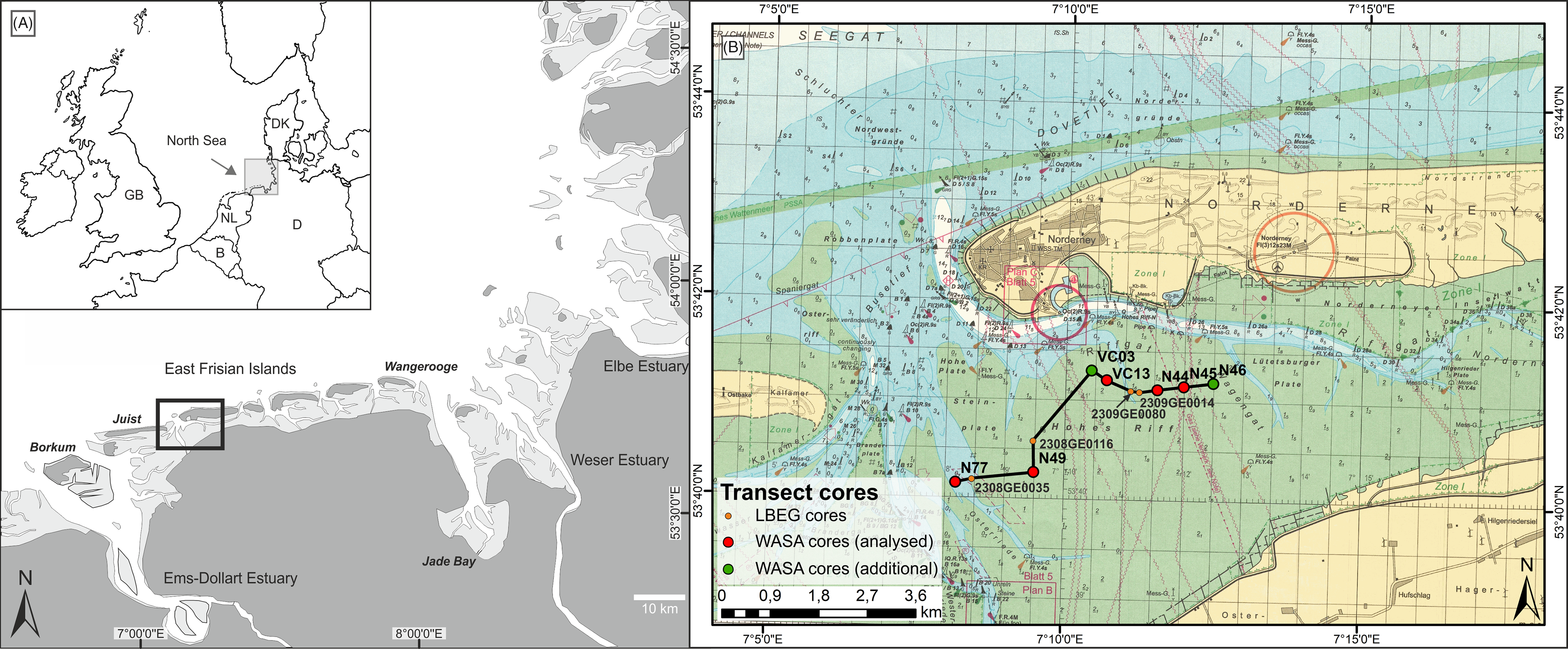
Fig. 1. Study area. (A) Overview of the North Sea coast with framed study area; (B) Investigated transect in the back-barrier of Norderney with investigated cores (red), additional WASA cores (green) and archive cores (orange). Map source: BMS (2016).
The sedimentary record is directly related to the Holocene sea-level rise. After the LGM ~21 ka BP, a strong eustatic sea-level rise (Clark et al., Reference Clark, Dyke, Shakun, Carlson, Clark, Wohlfarth, Mitrovica, Hostetler and McCabe2009) started as a consequence of the melting of the Fennoscandian and Laurentide ice sheets. The increase in free water as well as the glacio-isostatic adjustment led to a sea-level rise of 110 to 130 m which resulted in a lateral shift of the North Sea coast of c.600 km to the south (Kiden et al., Reference Kiden, Denys and Johnston2002; Behre, Reference Behre2004; Streif, Reference Streif2004).
The East Frisian Islands have formed since ~7–6 ka BP (Flemming, Reference Flemming, Wefer, Berger, Behre and Jansen2002), when sea-level rise slowly decelerated. With continuing RSL rise and prevalent current direction they have continuously migrated southeastward. The tidal flats also formed after the deceleration of the RSL rise around 6–7 ka BP when the North Sea reached the position of the present-day Wadden Sea (e.g. Flemming, Reference Flemming, Wefer, Berger, Behre and Jansen2002; Streif, Reference Streif2004; Behre, Reference Behre2007). The tidal range increased when the southern and northern North Sea merged and as a consequence the tidal flats expanded. Subsequently, Holocene peat deposits and siliciclastic sediments accumulated on top of the Pleistocene sands, reaching thicknesses of up to 25 m (Streif, Reference Streif2004). Peat layers intercalated in the marine sediments of the Holocene sequence are interpreted as temporary changes of rates of RSL rise and accelerated sediment supply causing regressive phases in the sense of a coastal progradation (Freund & Streif, Reference Freund and Streif2000; Streif, Reference Streif2004). The tidal-flat sediments consist 90% of reworked Pleistocene sediments, and only 10% of recently transported fluvial material (Hoselmann & Streif, Reference Hoselmann and Streif1997).
The marshlands are defined as the terrestrial area bordering the sea (Streif, Reference Streif1998). Two different types of marshland are distinguished: the salt marshes and the diked areas (Streif, Reference Streif1990). The salt marshes formed on nutrient-rich silt deposits above the mean high tide level. They are inundated and supplied with sediments only during spring-tide and storm-surge events.
In the Netherlands, human interference with the coastline started in the late Iron Age/Roman period. The development of the Wadden Sea is subject to intense anthropogenic influences, at latest since the construction of a continuous dyke system along the Frisian coast in the 13th century. This leads to a strong reworking of the tidal-flat sediments (Van der Spek, Reference Van der Spek1996), a process known as Wadden Sea Squeeze, which results in the loss of mudflats (Reineck & Siefert, Reference Reineck and Siefert1980; Flemming & Nyandwi, Reference Flemming and Nyandwi1994; Mai & Bartholomä, Reference Mai and Bartholomä2000). The long-term consequences of these influences are not conceivable in detail but will affect the stability, persistence and preservation of this unique UNESCO World Heritage Site.
Study site
Norderney is one of the East Frisian barrier islands of the German North Sea coast, lying c.4.5 km north of the mainland. The East Frisian barrier islands build an island chain in a mesotidal regime protecting the back-barrier tidal flats and the mainland from the direct influence of waves and storm surges. The tidal range at Norderney is 2.5 m (BSH, 2019). The tidal flats exhibit a shore-normal energy gradient resulting in an overall succession from sand flats in the north, to mixed flats and finally mudflats in the south directly bordering the mainland coast (Nyandwi & Flemming, Reference Nyandwi and Flemming1995). The analysed ~6 km long west–east transect is situated in the back-barrier of Norderney. In the west, it starts at the main tidal inlet, ‘Norderneyer Seegat’, crossing the sandbank ‘Hohes Riff’ to the northeast up to the ‘Norderneyer Wattfahrwasser’ directly south of the island (Fig. 1). According to the maps by Homeier (Reference Homeier1964), the positions of the ‘Norderneyer Seegat’ and the ‘Hohes Riff’ were relatively stable during the previous 400 years.
Methods
Fieldwork
Five sediment cores were collected in different environments. The investigated sediment cores (N77, N49, VC13, N44, N45) were obtained as part of the WASA project, using different coring techniques. Tidal-channel cores were conducted from the research vessel MS Burchana using a vibrocorer VGK-6 (VC-6000, med consultans GmbH) and plastic liners with 10 cm diameter, whereas tidal-flat cores were conducted using a vibrocorer (Wacker Neuson IE high-frequency vibrator head and generator) and aluminium liners with 8 cm diameter.
The geographic position of the drill sites was determined by a differential GPS with a cm-range accuracy. The elevation data were obtained with reference to the German standard elevation zero (NHN).
Opening, photographic documentation and macroscopic core description after Preuss et al. (Reference Preuss, Vinken and Voss1991) was performed at the Lower Saxony Institute for Historical Coastal Research in Wilhelmshaven, Germany, and the Institute of Geography of the University of Bremen, Germany. Samples for sedimentological and microfaunal analyses were taken along a 10 or 20 cm grid, including some additional samples for smaller-scale layers.
Laboratory analyses
In order to determine depositional processes, sedimentological, geochemical and microfaunal investigations were conducted for 84 samples from the five sediment cores. A special focus was laid on the identification of microfauna associations enabling conclusions on ecological conditions, thus supporting or adjusting facies interpretation. Sedimentological and geochemical analysis concentrated on the grain-size distribution and on nitrogen (N) and carbon content (total organic carbon = TOC, total inorganic carbon = TIC). These analyses helped to further classify the facies. Multivariate statistics (PCA) were performed to support the interpretation and identify controlling environmental factors.
For sedimentological and geochemical investigations, the sample material was dried at 40°C and carefully pestled by hand. For grain-size analysis, carbonate was removed by adding hydrochloric acid (HCl, 10%) and the organic components were removed using hydrogen peroxide (H2O2, 15%) (Blume et al., Reference Blume, Stahr and Leinweber2011). In order to prevent aggregation, sample material was treated with sodium pyrophosphate (Na4P2O7; 46 g l−1). The grain-size distribution was measured for the fraction between 0.04 µm and 2 mm using a laser particle size analyser (Beckmann Coulter LS13320; laser beam 780 nm) applying the Fraunhofer optical mode (Eshel et al., Reference Eshel, Levy, Mingelgrin and Singer2004). The grain-size distribution provides important information on hydro-energetic levels and the depositional environment. Furthermore, microfaunal associations can be related to the grain-size distribution, since different species prefer different substrates (Blott & Pye, Reference Blott and Pye2001; Frenzel et al., Reference Frenzel, Keyser and Viehberg2010).
The concentrations of N, TOC (accounting for c.50% of the organic matter) and total carbon (TC) within the samples were measured after grinding the samples using an elemental analyser (elementar, Vario EL Cube). For TOC measurements, carbonates were removed by the addition of HCl (10%) (Pribyl, Reference Pribyl2010). This enabled the determination of TIC, accounting for c.12% of the calcium carbonate (CaCO3), from the difference of TC and TOC (Bernard et al., Reference Bernard, Bernard and Brooks1995). Finally, the C/N ratio was derived providing information about the origin of organic matter (Last & Smol, Reference Last and Smol2002; Khan et al., Reference Khan, Vans, Horton, Shennan, Long and Horton2015).
Microfauna samples were carefully shaken overnight, using a dispersant (sodium pyrophosphate; Na4P2O7; 46 g l−1) to prevent clay adhesion, and washed through sieves (63 and 100 µm) in order to isolate microfossils (>100 µm) from fine-grained sediment. Where possible, 100 individuals were counted dry, however, accepting a minimum of 40 individuals for samples with very low abundance (cf. Scheder et al., Reference Scheder, Frenzel, Bungenstock, Engel, Brückner and Pint2019). Analysed and residual material was weighed to enable extrapolation and calculation of microfaunal concentration. Species determination followed taxonomic descriptions and illustrations in Athersuch et al. (Reference Athersuch, Horne and Whittaker1989), Gehrels & Newman (Reference Gehrels and Newman2004), Horton & Edwards (Reference Horton and Edwards2006), Murray (Reference Murray2006) and Frenzel et al. (Reference Frenzel, Keyser and Viehberg2010). The replacement of Elphidium excavatum by Cribroelphidium excavatum (Terquem, 1875) as well as the replacement of Pontocythere elongata by Cushmanidea elongata (Brady, 1868) was adopted according to the online database WORMS. Due to problematic discrimination and low counts of individuals of (Cribro-)Elphidium (e.g. Elphidium cuvillieri and Cribroelphidium gunteri), these species were grouped under Elphidium spp. for counting. Furthermore, occurring species of Leptocythere were grouped under Leptocythere spp. for counting, due to the problematic discrimination of juvenile individuals.
Radiocarbon (14C) age determination
A chronological framework is provided by 13 age determinations originating from the sediment cores N77, N49, VC13 and N44 (Table 1). The 14C age determinations (accelerator mass spectrometry (AMS)) were performed by the Poznań Radiocarbon Laboratory (Poland). The results were calibrated with the software CALIB (Version 7.1) using the calibration curves IntCal13 and Marine13 (Reimer et al., Reference Reimer, Bard, Bayliss, Beck, Blackwell, Ramsey, Buck, Cheng, Edwards, Friedrich, Grootes, Guilderson, Haflidason, Hajdas, Hatté, Heaton, Hoffmann, Hogg, Hughen, Kaiser, Kromer, Manning, Niu, Reimer, Richards, Scott, Southon, Staff, Turnex and van der Plicht2013). According to measurements of Enters et al. (Reference Enters, Haynert, Wehrmann, Freund and Schlütz2020) the ΔR value for reservoir correction of ages originating from in situ shell material was presumed 74 ± 16 14C years.
Table 1. Radiocarbon ages calibrated with IntCal13, dataset 1 (for northern hemisphere terrestrial 14C dates) and Marine13 (for mollusc dating, sample Poz-97990) with reservoir correction (delta R 74 ± 16) after Enters et al. (Reference Enters, Haynert, Wehrmann, Freund and Schlütz2020).

a Ph. australis, C. vulgaris and E. tetralix vegetative remains, C. mariscus, Schoenoplectus and P. anserina fruits and seeds.
b Exact age data after calibration.
Data processing
Measures for univariate statistical grain size were calculated by means of the Excel tool GRADISTAT (Version 4.0) (Blott & Pye, Reference Blott and Pye2001), after Folk & Ward (Reference Folk and Ward1957). A correlation analysis (Spearman’s rs) allowed detection of relationships between the different parameters (sand amount, mean grain size, TOC, TIC and C/N) and of possible autocorrelations. Microfauna distributions and environmental parameters were analysed by means of multivariate statistics (principal component analysis (PCA)) in order to find driving environmental factors and support the facies interpretation. PCA was only performed on samples with a complete dataset of all three analyses using the software PAST (v. 3.2.1) (Hammer et al., Reference Hammer, Harper and Ryan2001).
Results and interpretation
Lithological units
Six lithological units (A–F) were identified based on foraminifer and ostracod associations, visual features in the sediment cores, grain-size distribution and TOC, TIC and N content. However, not all units are present in all sediment cores (Figs. 3 and 4 further below; Supplementary Figs S1–S3 (in the Supplementary Material available online at https://doi.org/10.1017/njg.2020.16)). Nine foraminifer taxa and 11 ostracod taxa were identified (Fig. 2; Supplementary Table S1 (in the Supplementary Material available online at https://doi.org/10.1017/njg.2020.16)).
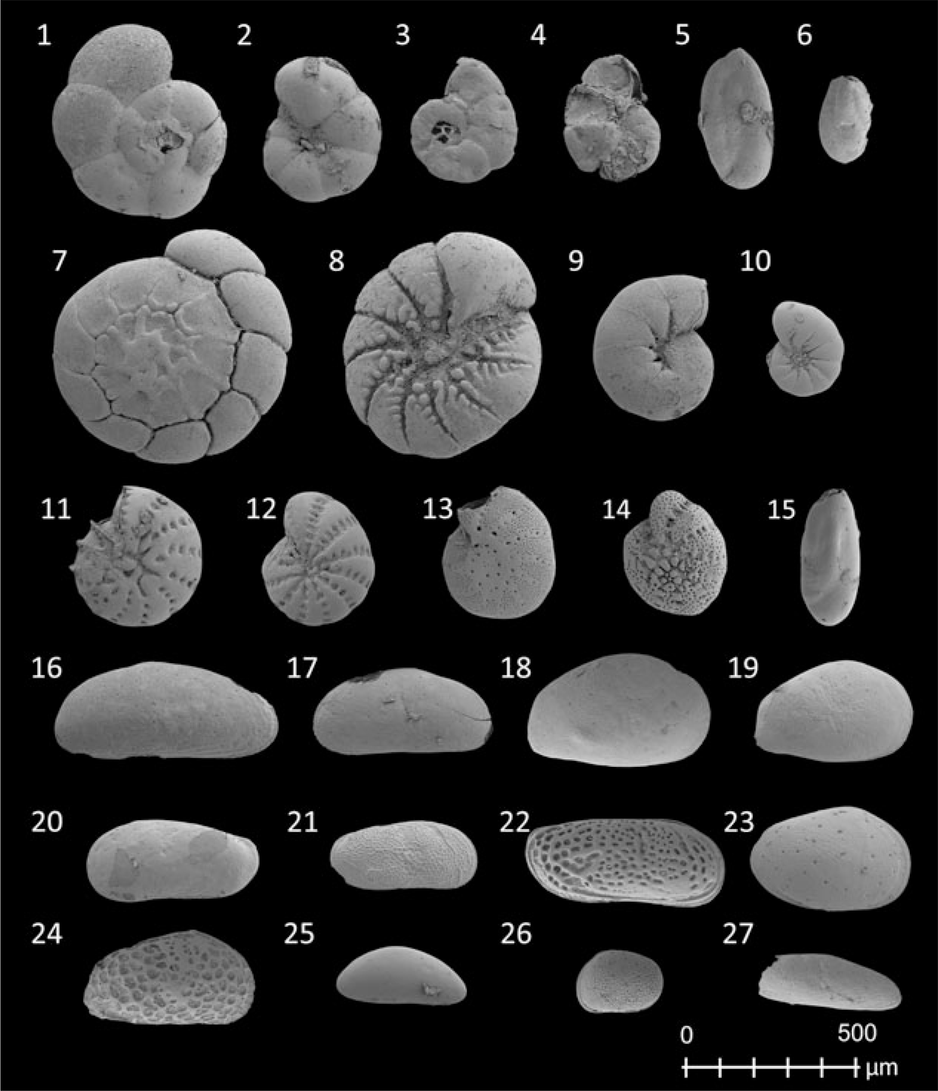
Fig. 2. Scanning electron microscope (SEM) images of frequently documented foraminifera (1–15) and ostracod (16–27). 1–2: Trochammina inflata (Montagu, 1808); 3–4: Entzia macrescens (Brady, 1870); 5–6: Miliammina fusca (Brady, 1870); 7–8: Ammonia tepida (Cushman, 1926); 9–10: Haynesina germanica (Ehrenberg, 1840); 11–12: Cribroelphidium williamsoni (Haynes, 1973); 13: Elphidium cuvillieri (Levy, 1966); 14: Cribroelphidium gunteri (Cole, 1931); 15: Triloculina oblonga (Montagu, 1803); 16: Cushmanidea elongata (Brady, 1868); 17: Cushmanidea elongata (Brady, 1868), juvenile, 18–19: Cyprideis torosa (Jones, 1850), juvenile; 20: Leptocythere lacertosa (Hirschmann, 1912), juvenile; 21: Leptocythere castanea (Sars, 1866), juvenile; 22: Leptocythere pellucida (Baird, 1850); 23: Loxoconcha elliptica (Brady, 1868), juvenile; 24: Urocythereis britannica (Athersuch, 1977), juvenile; 25: Cytherois cf. pusilla (Sars, 1928), juvenile; 26: Hirschmannia viridis (Mueller, 1785), juvenile; 27: Sahnicythere retroflexa (Klie, 1936), juvenile.

Fig. 3. Sedimentological, geochemical and microfaunal results of N77, including the most relevant component of the PCA.
Fig. 4. Sedimentological, geochemical and microfaunal results of N49, including the most relevant component of the PCA. For the colour legend see Figure 3.
Unit A: Pleistocene deposits
Unit A is characterised by moderately well to well-sorted fine sand and was exclusively documented in N77 (7.75–4.95 m below NHN) (Fig. 3). TOC, TIC and N measurements are below the detection limit. Therefore, the C/N ratio is not regarded as significant as it varies around transitional values between aquatic and terrestrial environments (e.g. Last & Smol, Reference Last and Smol2002; Khan et al., Reference Khan, Vans, Horton, Shennan, Long and Horton2015). The entire unit is void of microfauna, which indicates a terrestrial environment. Since the study area was subject to periglacial conditions, with accumulation of aeolian and glaciofluvial sands (cf. Streif, Reference Streif2004), Unit A is assumed to represent Pleistocene/Geest deposit.
Unit B: palaeosol
Unit B is characterised by moderately well-sorted fine sand and also occurs exclusively in core N77 (4.95–4.41 m below NHN). Macroscopic core description shows dark laminae which seem richer in organic matter than Unit A. However, TOC contents are below the detection limit, permitting verification of higher organic contents. Since N also remains below the detection limit, the C/N ratio, indicating a terrestrial origin of the organic matter (Last & Smol, Reference Last and Smol2002; Khan et al., Reference Khan, Vans, Horton, Shennan, Long and Horton2015), is again not significant. Observations of Bulian et al. (Reference Bulian, Enters, Schlütz, Scheder, Blume, Zolitschka and Bittmann2019) from a core in the vicinity show signs of pedogenesis for a comparable layer. Together with the macroscopic core description, this leads to the assumption that Unit B represents a palaeosol at the base of the Holocene sedimentary sequence (Holocene base).
Unit C: peat
Unit C is characterised by dark brown organic deposits containing layers of clastic material with moderately well-sorted fine sand and poorly sorted sandy mud. It was documented in four cores (N77: 4.41–3.68 m below NHN; VC13: 3.76–3.73 m below NHN; N44: 3.786–3.24 m below NHN; and N49: C-1: 4.42–4.17 m; C-2: 3.37–3.0 m below NHN). Since no sample material was available from Unit C in VC13, the identification here is based on the macroscopic core description. TOC contents increase in all cores, representing the maximum (between ~30% and ~40%) of the respective core. A similar pattern is documented for N contents (maximum values around 1.6%). For C-2 (N49) both values increase but do not reach similarly high values. TIC is considerably low except for N77 and N49 (C-2), where it increases to ~35% and ~10%. C/N ratios and the lack of microfauna point to a semi-terrestrial environment in most samples. Together, these results indicate the formation of a peat, with high organic contents due to decaying vegetation and low carbonate contents resulting from decalcification processes associated with peat formation (Bungenstock Reference Bungenstock2005; Scheder et al., Reference Scheder, Engel, Bungenstock, Pint, Siegmüller, Schwank and Brückner2018). The locally higher TIC values (N77 and N49 C-2) may indicate an increased marine influence. For N77 this is in accordance with several intercalated fine-grained layers indicating episodic marine inundations. For N49 (C-2), the slightly increased TIC content possibly results from bioturbation at the erosive contact (Bird, Reference Bird2008). The foraminifers occurring in C-1 (N49) are mainly characterised by agglutinated Trochammina inflata (Montagu, 1808), Entzia macrescens (Brady, 1870) and Miliammina fusca (Brady, 1870). These typical salt-marsh species were either introduced by relocation or by post-depositional bioturbation (Athersuch et al., Reference Athersuch, Horne and Whittaker1989; Murray, Reference Murray2006) or alternatively, they indicate a transition to the overlying deposit. The fen peat in N49 (C-1), VC13 and N44 formed directly on top of the Geest deposits and is therefore referred to as basal peat. Samples from N77, N49 (C-1) and N44 provided 14C ages for the upper parts of the basal peat (Table 1); in the west (N77) it dates to 7170–6950 cal BP (bottom) and 5890–5660 cal BP (top), whereas towards the east (N49) it dates to 4850–4630 cal BP and 3980–3730 cal BP (N44). The bottom of the second peat in N49 (C-2) dates to 4350–4010 cal BP and the top shows an age of 4520–4260 cal BP directly below the erosional contact.
Unit D: salt-marsh deposits
Unit D is characterised by poorly sorted sandy mud to muddy sand and was documented in four cores (N77: 3.68–3.32 m below NHN; N49: 4.17–3.37 m below NHN; VC13: 3.73–2.87 m below NHN; and N44: 3.24–2.895 m below NHN). The geochemical parameters vary strongly between the cores. While TIC, TOC and N values in N49 are very low, TOC and N values in N77 decrease but are still considerably high, whereas no TIC is documented. Furthermore, in VC13, TOC and N show high values, whereas TIC strongly decreases upwards. N44 shows a reversed pattern (increasing TIC, decreasing TOC and N. C/N ratios vary between >5 and ~20, indicating a transitional environment between terrestrial and aquatic conditions (cf. Last & Smol, Reference Last and Smol2002; Khan et al., Reference Khan, Vans, Horton, Shennan, Long and Horton2015). However, the presence of salt-marsh foraminifers, which are almost exclusively T. inflata and E. macrescens, indicates a more aquatic environment. Unit D is identified as salt-marsh deposit based on the documented C/N ratios, the microfaunal association and the typical poorly sorted, fine-grained sediments (Bakker et al., Reference Bakker, Bos, Stahl, Vries and Jensen2003). The lack of microfauna in N77 is interpreted as a very low inundation frequency resulting from the distance from the coastline which defines the upper limit of the high salt marsh. An alternative explanation is that microfauna was destroyed after the deposition of the layer or dissolved by humic acids of plant decomposition (Bungenstock, Reference Bungenstock2005; Scheder et al., Reference Scheder, Engel, Bungenstock, Pint, Siegmüller, Schwank and Brückner2018). The top of the salt-marsh deposits in VC13 and N44 is erosive. Salt-marsh samples from N77 (top), VC13 (bottom and top) and N44 (top) were dated (Table 1), providing the oldest age of 5580–5320 cal BP in the west (N77). The base of Unit D in VC13 dates to 4810–4450 cal BP, and the top dates to 4080–3900 cal BP, whereas the top in N44 shows ages of 3680–3480 cal BP and 3980–3730 cal BP.
Unit E: channel deposits
Unit E is characterised by (very) poorly sorted muddy sand and was documented in three cores (N77: 3.32–2.98 m below NHN; N44: 2.895–2.245 m below NHN; and N45: 6.21–2.70 m below NHN). TOC, TIC and N values are considerably low in all samples and the low C/N ratios indicate an aquatic environment. The poor sorting, with sand as main grain-size component, and the low nutrient contents point to a marine channel with low energy levels, where fine-grained sediments are deposited due to meandering (Zepp, Reference Zepp2017). The microfauna supports this interpretation, as occurring salt-marsh species (N77) indicate relocation (Horton & Edwards, Reference Horton and Edwards2006; Murray, Reference Murray2006) and were possibly redistributed by the typical erosion–accumulation pattern of meandering channels (cf. Zepp, Reference Zepp2017). The microfauna concentration in N44 is generally high, with lower abundances in the sandier (higher-energy) parts. The layer shows very great diversity, with shallow marine species clearly dominating. As such were identified mainly Ammonia tepida (Cushman, 1926) and Haynesina germanica (Ehrenberg, 1840), accompanied by Cribroelphidium williamsoni (Haynes, 1973), Leptocythere (Sars, 1925) and taxa of lower abundance (Athersuch et al., Reference Athersuch, Horne and Whittaker1989; Horton & Edwards, Reference Horton and Edwards2006; Murray, Reference Murray2006; Frenzel et al., Reference Frenzel, Keyser and Viehberg2010). This dominance of shallow marine species supports the interpretation that Unit E represents a low-energy channel.
Unit F: tidal-flat deposits
Unit F is characterised by poorly sorted muddy sand gradually changing upwards to very well-sorted fine sand and was documented in four cores (N49: 3.0–0.98 m below NHN; VC13: 2.87–0.73 m below NHN; N44: 2.245–0.795 m below NHN; and N45: 2.70–0.53 m below NHN). The top of this unit represents the sediment surface in these cores. For N49 and N44, only microfaunal data are available, in addition to the macroscopic description, due to lack of material. The good sorting and the high dominance of fine sand indicate a higher energy level compared to Units C–D (Wartenberg et al., Reference Wartenberg, Vött, Freund, Hadler, Freche, Willershäuser, Schnaidt, Fischer and Obrocki2013). Unit F exhibits subunits in all sediment cores, which are characterised by coarser-grained deposits, indicating a short-term high-energy event, such as a storm surge (Wartenberg et al., Reference Wartenberg, Vött, Freund, Hadler, Freche, Willershäuser, Schnaidt, Fischer and Obrocki2013). TOC and N lie at considerably low levels and are below the detection limit in VC13. The C/N ratio varies but mainly indicates aquatic conditions (N45). The present mollusc fragments and the intercalated coarser layers support this interpretation. The microfauna concentration in Unit F varies between <100 and ~8000 Ind./10 cm3 (individuals per 10 cm³), which is possibly connected to variations in grain-size distribution representing energy levels, and TOC and N contents representing nutrient availability. One peak is documented for the microfauna concentration at the base of Unit F in VC13, which is interpreted as reworking due to the erosive contact between units D and E. A. tepida mainly dominates over H. germanica. This indicates a lower salinity, as A. tepida has its optimum at lower salinities (Murray, Reference Murray2006). H. germanica dominates over A. tepida only in the uppermost samples of N44 and VC13, indicating an increasing salinity. Besides these two most common species, shallow marine foraminifer and ostracod taxa occur. All this leads to the interpretation of Unit F as a tidal-flat environment. The very few documented salt-marsh foraminifers are interpreted as introduced by the tidal current. The articulated bivalve Barnea candida (Linnaeus, 1758) in living position is documented directly at the erosional contact between the tidal flat and the underlying peat in N49 (Fig. 4). It is positioned inside its borehole and dates to 910–730 cal BP.
Evaluation and interpretation of the fossil data
In order to find variables accounting for as much of the variance in the dataset as possible (Davis, Reference Davis1986; Harper, Reference Harper1999), the foraminifer and osctracod associations as well as the environmental parameters were analysed by means of a PCA. This analysis should enable the identification of driving environmental factors and support the facies interpretation.
After the calculation of Spearman’s correlation coefficients, parameters showing auto- or very high correlations were excluded from the dataset. Very rare (<5%) taxa of foraminifers and ostracods were also excluded. Subsequently, the PCA was performed separately for each sediment core as well as jointly for all sediment cores, including the parameters sand amount, TOC, TIC, C/N and the microfaunal associations. The results (Figs 5–7; Supplementary Figs S4–S7 (in the Supplementary Material available online at https://doi.org/10.1017/njg.2020.16)) confirm the identified units based on the revealed sample groupings. In all PCAs, PC 1 and 2 are the most relevant components, whereas PC 3 shows variances of less than 10%.
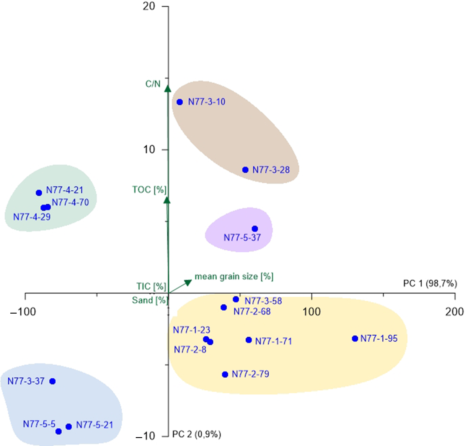
Fig. 5. PCA biplot of N77 showing the two most relevant axes (PC 1 and PC 2). Colours of sample groupings relate to the colour legend in Figure 3; green arrows represent environmental parameters and blue points represent samples.
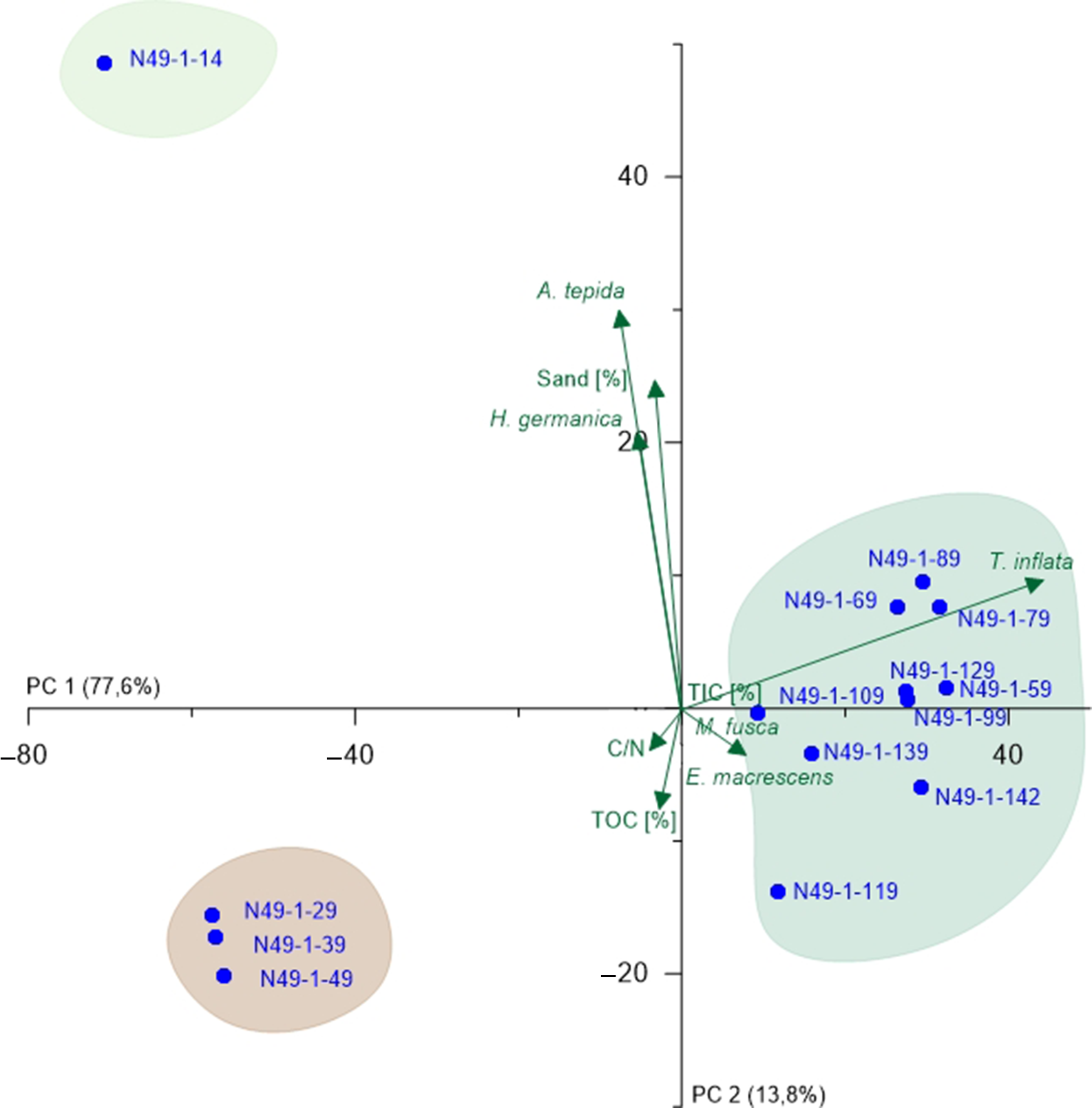
Fig. 6. PCA biplot of N49 (lower part) showing the two most relevant axes (PC 1 and PC 2). Colours of sample groupings relate to the colour legend in Figure 3; green arrows represent microfaunal taxa and environmental parameters, and blue points represent samples.

Fig. 7. PCA biplot of all cores, showing the two most relevant axes (PC 1 and PC 2). Colours of sample groupings relate to the colour legend in Figure 3; green arrows represent microfaunal taxa and environmental parameters, and coloured points represent samples.
For N77, the PCA was carried out without microfauna, as there were only two samples containing the latter (Fig. 5). PC 1 (98.7%) opposes samples with higher TIC contents (negative values) and those with TIC values below the detection limit (positive values) suggesting that PC 1 represents a factor driven by marine influence possibly connected to water depth (Bird, Reference Bird2008). This component shows a very high variance, which makes PC 2 (0.9%) insignificant. Nevertheless, it is clearly opposing TOC content (positive values) and sand amount (negative values). Since the deposition of organic matter is strongly dependent on hydrodynamic levels, a grain-size factor is assumed for PC 2 (Khan et al., Reference Khan, Vans, Horton, Shennan, Long and Horton2015). The different sample groupings (Fig. 5) are mainly associated to the identified units (A, C, D and E), whereas the salt-marsh samples (Unit D) form the most distinct group.
For N49, two PCAs were carried out, one including the lower half of the core with all performed analyses, and one for the upper half with exclusively microfauna (Fig. 6; Supplementary Fig. S4 (in the Supplementary Material available online at https://doi.org/10.1017/njg.2020.16)). In both cases, PC 1 does not outnumber PC 2 as intensely as in N77. For the lower core (Fig. 6), PC 1 (77.6%) opposes all salt-marsh samples together with the typical salt-marsh species (positive values) and mainly peat and shallow marine species (negative values) indicating a marine-influence factor, whereby the peat samples distort the results here. Comparison of the ecological preferences of the opposed species leads to the assumption that PC 1 represents salinity (Murray, Reference Murray2006). PC 2 (13.8%) opposes sand amount (positive values) and TOC content (negative values), again suggesting a grain-size component. However, due to the preference of A. tepida and H. germanica for rather fine-grained material, which hints at reworking effects, uncertainties remain. Again, the groupings reflect the previously defined units (C, D and F). For the upper half (Supplementary Fig. S4 (in the Supplementary Material available online at https://doi.org/10.1017/njg.2020.16)), PC 1 (63.2%) opposes A. tepida and H. germanica, which hints at the salinity. This is based on the fact that A. tepida dominating over H. germanica indicates a lower salinity (Murray, Reference Murray2006). PC 2 (32%) is much stronger than in the lower core half and opposes the two mentioned species and all other taxa, especially C. williamsoni. Since the latter prefers substrates with clay- and mud contents <60%, whereas A. tepida and H. germanica prefer clay- and mud contents >80% (Murray, Reference Murray2006), this component is interpreted to represent the grain size. Only one group is visible in the PCA plot (Supplementary Fig. S4 (in the Supplementary Material available online at https://doi.org/10.1017/njg.2020.16)) apparently associated to H. germanica, suggesting an influence of slightly increased salinity for this part of the tidal-flat deposits (Murray, Reference Murray2006). Considering both partial PCAs, salinity plays a major role for the complete core, whereas the grain size is more important in the upper than in the lower half.
The PCA plots of the other cores are documented in Supplementary Figures S5–S7 (in the Supplementary Material available online at https://doi.org/10.1017/njg.2020.16). For VC13, PC 1 (76.8%) is interpreted as a water-depth factor, whereas PC 2 (12.3%) represents the general marine influence. N44 is influenced by the grain size as the first component (PC 1; 63.9%) and the marine influence as the second (PC 2; 23.1%). N45 is mainly driven by the grain size (PC 1; 87.0%) and to a lesser extent by water depth and/or salinity (PC 2; 8.7%). The joint PCA (Fig. 7) is highly influenced by the presence or absence of microfauna, leading to a relatively good separation of shallow-marine (Units E and F), mainly supratidal to semi-terrestrial (Units C and D) and mainly semi-terrestrial to terrestrial (Units A, B and C) environments (Fig. 7). PC 1 (36.9%) is likely related to the grain size due to the strong approximation of the sand amount to the first axis. PC 2 (11.9%) opposes salt-marsh species (and samples) and TIC content with TOC content and more terrestrial samples suggesting a general marine-influence factor.
Correlation
The analysed cores were complemented by two additional WASA cores (VC03 and N46) and four archive cores of the LBEG (2308GE0035, 2308GE116, 2309GE0080, 2309GE0014), in order to enable the correlation of the layers identified and their respective facies. The transect reaches from the ‘Norderneyer Seegatt’ at the western tip of Norderney 6 km to the east directly south of the Norderney island tidal channel (Fig. 8). Since only one core reaches the Pleistocene deposits, the Holocene base was modelled based on the geological coastal map of the LBEG (2019), accessed through the ‘NIBIS® Kartenserver’.

The integration of the LBEG cores in our stratigraphic cross-section requires critical analysis of the archive core descriptions. The descriptions are often not detailed enough for a reliable landscape reconstruction, as the LBEG cores were conducted for different purposes, e.g. engineering or hydrogeology, and by different processors. Therefore, facies interpretations were reviewed based on the knowledge gained from the WASA cores (cf. Scheder et al., Reference Scheder, Frenzel, Bungenstock, Engel, Brückner and Pint2019). With that, integrating them in the profile section helps to obtain a more precise picture of facies successions in the study area.
The sedimentation history in the study area can be reconstructed starting with the deposition of late Pleistocene sands. These were documented in the western part of the study area (N77) and identified based on the grain-size distribution and the lack of organic and inorganic carbon as well as missing microfauna. The latter indicates a non-aquatic habitat, supporting the interpretation as late Pleistocene. We assign the last glacial period, locally known as Weichselian. The study area was subject to periglacial conditions where aeolian and glaciofluvial processes dominated (Streif, Reference Streif2004). The top of these deposits shows higher C/N ratios pointing to terrestrial conditions (Khan et al., Reference Khan, Vans, Horton, Shennan, Long and Horton2015), but inconclusively as the counts of C and N are low (N77, chapter 4). The terrestrial origin is clear in VVC17, as decomposition of organic matter indicates the formation of a palaeosol on top of the aeolian and glaciofluvial sands (Bulian et al., Reference Bulian, Enters, Schlütz, Scheder, Blume, Zolitschka and Bittmann2019).
Subsequently, a fen peat developed, marking the base of the Holocene sequence. The dating results indicate spatial differences in peat formation and a time-transgressive development. In the western part, peat formation started ~7500 cal BP and lasted for ~1500 years (VVC17), whereas to the east, peat formation is documented with an age of ~4700 cal BP in the upper part of the basal peat in N49. This is regarded as a minimum age, as the base of the peat was not reached. The time-transgressive nature of the peat formation reflects the rising groundwater level associated with the RSL rise (e.g. Vink et al., Reference Vink, Steffen, Reinhardt and Kaufmann2007; Baeteman et al., Reference Baeteman, Waller and Kiden2011). Furthermore, the area became protected ~6–7 ka BP by the developing barrier island, maintaining sheltered conditions for peat growth during a rising RSL (Freund & Streif, Reference Freund and Streif2000; Flemming, Reference Flemming, Wefer, Berger, Behre and Jansen2002; Bungenstock & Schäfer, Reference Bungenstock and Schäfer2009). Foraminifers and marine diatoms in the upper parts of the peat suggest an increasing marine influence.
The increasing marine influence resulted in the development of a salt marsh burying the basal peat. This interpretation is based on the microfaunal association, consisting of typical salt-marsh species, especially T. inflata and E. macrescens. The grain-size distribution indicates a low-energy environment, and C/N ratios vary between aquatic and semi-terrestrial conditions (Horton and Edwards, Reference Horton and Edwards2006; Khan et al., Reference Khan, Vans, Horton, Shennan, Long and Horton2015). The 14C age data prove the initiation of salt-marsh formation ~6000 cal BP in the west (N77), whereas to the east it started to develop after ~4700 cal BP. This is explained by the palaeogeographic situation of the forming barrier island, which provided shelter for the more easterly part, leading to a delay in salt-marsh formation. However, an influence of relocation of the dated material in N77 (Table 1) has to be considered. Since the salt-marsh deposits documented in the adjacent core VVC17 (Bulian et al., Reference Bulian, Enters, Schlütz, Scheder, Blume, Zolitschka and Bittmann2019) are of approximately the same age but are situated ~2 m deeper than in N77, a correlation of both layers is difficult, supporting the assumption of relocation in N77.
An intercalated peat in the west was documented in core VVC17, with peat growth dated from ~5900 to 5300 cal BP. It remains undetermined whether this indicates a regression (Baeteman Reference Baeteman1999; Bungenstock & Weerts, Reference Bungenstock and Weerts2010, Reference Bungenstock and Weerts2012).
An additional intercalated peat developed ~4300 cal BP on top of the salt marsh, documented in core N49). The top is characterised by an erosive contact. Erosional contacts are documented in three cores further east (VC03, VC13 after ~3900 cal BP and N44 after ~3600 cal BP), indicating a hiatus.
During that time, the main channel had already shifted to the western part of the study area, following the southeastward migration of the barrier islands (e.g. Flemming, Reference Flemming, Wefer, Berger, Behre and Jansen2002; Streif, Reference Streif2004). Salt-marsh species in the top layer of VVC17 indicate reworking and erosion, which appears as tidal-flat facies. East of the main channel, a tidal-flat environment developed as the result of rising RSL. Further to the east, this tidal flat was cut by another tidal channel, which was either infilled subsequently or shifted its location. An intercalated coarse-grained layer with abundant macrofaunal remains, which is correlated over three cores (N49, VC03 VC13), cuts the tidal-flat deposit laterally. We interpret this layer to represent either a high-energy event or a period of increased storm activity. The dating results prove a deposition after ~3600 cal BP. The overlying deposits show further coarse-grained layers, which indicates that higher dynamic conditions established in the back-barrier tidal flat, lasting until today.
Discussion
Assumptions on the spatial extent of palaeo-salt marshes
Palaeogeographic maps for different time periods during the Holocene RSL rise, with a landward- as well as seaward-shifted coastline, are an important reference for models of coastal protection, future long-term coastal development and archaeological sites. Especially for archaeological research, the salt marshes play an important role. Whereas the lower parts, the pioneer zones, were not appropriate for settling, the highly silted-up parts of the upper salt marshes with their high biological productivity were very attractive for habitation (Vos & Knol, Reference Vos and Knol2015; Nieuwhof & Vos, Reference Nieuwhof and Vos2018).
Existing approaches for landscape reconstruction on the German North Sea coast are mainly based on the so-called ‘Küstenprofilkarten’ derived from the descriptions of the archive core data published by the LBEG (Streif, Reference Streif1998, Reference Streif2004; Goldhammer & Karle, Reference Goldhammer and Karle2015; Karle et al., Reference Karle, Frechen and Wehrmann2017). These reconstructions do not show any, or show only small, rims or patches of salt-marsh areas. Possibly, this is because salt-marsh deposits are not always clearly detectable in the cores and are deficiently described, especially in cores taken for engineering purposes. We assume that salt marshes exhibited a much wider spatial extent compared to the traditionally mapped areas, which are based on the archive core data (Vos & Knol, Reference Vos and Knol2015; Karle, Reference Karle2020; Vos et al., Reference Vos, van der Meulen, Weerts and Bazelmans2020;).
The anthropogenic influence on the present-day coastal landscape is very strong. Even before embankment, ditches connected the sea to the hinterland and drainage lowered the peat areas. Due to the dyke system, the coastline is static, with the consequences of Wadden Sea Squeeze (Flemming & Nyandwi, Reference Flemming and Nyandwi1994), intense reworking of the tidal flats (Van der Spek, Reference Van der Spek1996) and the loss of mudflats (Reineck & Siefert, Reference Reineck and Siefert1980; Mai & Bartholomä, Reference Mai and Bartholomä2000). A small coastal transition zone with salt marshes exists only as a remnant in the protected areas of the national park. The inner-dyke landscape is even more artificial. This impedes imagination of a former coastal landscape, as there is no modern analogue. This is especially true for the brackish and lagoonal deposits described in the archive cores and several publications (e.g. Streif, Reference Streif2004; Bungenstock & Schäfer, Reference Bungenstock and Schäfer2009; Wartenberg & Freund, Reference Wartenberg and Freund2012; Karle et al., Reference Karle, Frechen and Wehrmann2017). Streif (Reference Streif1990) describes widely distributed brackish areas with low tidal ranges as transition between marine environments and river-, lake- and swamp-dominated environments. For areas of the Unterems, the Krummhörn (western East Frisia) and Wilhelmshaven, even lagoonal deposits were documented by Streif (Reference Streif1971), Barckhausen & Streif (Reference Barckhausen and Streif1978) and Barckhausen (Reference Barckhausen1984). They describe clayey to silty deposits with up to 5% fine sand, which show very low to no carbonate content. The deposits exhibit a horizontal layering, with plant debris and Fe-sulphide aggregates. Both the brackish and the lagoonal sediments are deposited in a subaquatic, microtidal and low-saline environment (Streif, Reference Streif1990). However, predictions on changing tidal range during the Holocene RSL rise in the southern North Sea consistently show increases in tidal range since the early Holocene. The major changes occurred prior to 6 ka BP, and only minor (cm-scale) to no changes occurred subsequently (Shennan et al., Reference Shennan, Lambeck, Flather, Horton, McArthur, Innes, Lloyd, Rutherford and Wingfield2000; Van der Molen & De Swart, Reference Van der Molen and De Swart2001). This is in contrast to the deposition of microtidal-induced brackish and lagoonal deposits as described before. Therefore, it may be assumed that the brackish/lagoonal sediments were deposited locally and are typical of protected areas like the Ems–Dollart region or Jade Bay. There, the brackish and lagoonal environment is mainly controlled by the palaeogeographical situation, including bays and the transition to rivers and swamps, and not under direct influence of the tides.
However, several authors apply the brackish/lagoonal core description to take account of sediments deposited in a less dynamic environment close to a terrestrial environment (LBEG core descriptions; Streif Reference Streif2004; Bungenstock & Schäfer Reference Bungenstock and Schäfer2009; Karle et al., Reference Karle, Frechen and Wehrmann2017). Wartenberg et al. (Reference Wartenberg, Vött, Freund, Hadler, Freche, Willershäuser, Schnaidt, Fischer and Obrocki2013) classify the brackish/lagoonal deposits as quiet reach sediments. This facies allows both direct access to the open sea and a lagoon-type isolated palaeogeographical situation. In this way, depositional processes are described independently from a lagoonal landscape situation sensu stricto. Tidal–marine as well as limnic–terrestrial conditions may occur and locally salt marshes form (Wartenberg et al., Reference Wartenberg, Vött, Freund, Hadler, Freche, Willershäuser, Schnaidt, Fischer and Obrocki2013). As salt marshes are part of the supratidal area, stagnant water in ponds was present.
For the presented west–east transect in the back-barrier of Norderney, the fine-grained sediments showing a quiet-reach deposition in between and on top of the peat layers are clearly identified as salt-marsh deposits. They were deposited within a timespan between ~4500 cal BP and ~3300 cal BP in the largest part of the transect. The latter allows the correlation of these salt-marsh deposits over up to 5 km. A landscape reconstruction for this area, therefore, shows a wide and stable rim of salt marshes along the former coastline. This wide distribution defines them as a characteristic element of the palaeolandscape.
For the coast of the northern Netherlands, geoarchaeological research has revealed that salt marshes were inhabited after having reached a minimum thickness of 80 cm and an elevation with less than ~50 days of inundation per year (Vos, Reference Vos and Besteman1999; Vos & Gerrets, Reference Vos and Gerrets2004). The habitation of the salt-marsh region in the Netherlands started around 2700 cal BP (Taayke, Reference Taayke and Nieuwhof2016) directly on the high marshes and later on salt-marsh ridges or levees that had reached the level of only a middle marsh (Vos, Reference Vos and Besteman1999, Reference Vos2015; Vos & Gerrets, Reference Vos and Gerrets2004). Due to the higher tidal range in the tidal basin of Norderney, for this area a thickness of c.1 m for salt marshes can be expected to enable settlement or at least human activity. Applying this information on the presented core transect, the western part of the sand plate ‘Hohes Riff’ (from N77 in the west to VC13, only interrupted in VC03 by strong erosion) has the potential for buried settlement remains with a minimum age of ~4000 cal BP. So far, no settlements of this age are known in the marshland areas of the German North Sea coast. The oldest known marshland settlement is Rodenkirchen, situated in the river marshes of the Weser and dating to ~3000 cal BP (Strahl, Reference Strahl2005). Therefore, further mapping of the extent of internal structure of the salt-marsh deposits in the back-barrier area of Norderney could give further information on the potential for human activity.
What triggers landscape change? Sea-level rise versus single events versus anthropogenic influence?
The sedimentary record shows an erosional contact on top of the peat and salt-marsh deposits of N49, VC03 and VC13. It extends over more than 3 km and is followed by a drastic change in depositional environment, suggesting a significant hiatus. In all three cores, the top of the peat is eroded and boreholes of B. candida are documented in the topmost part of the peat. In N49 an articulated adult individual of B. candida was documented inside its borehole. The adult species digs c.15 cm into soft substrates such as peat (Richter & Rumohr Reference Richter and Rumohr1976; National Museum Wales, 2016). It typically occurs from the lower intertidal to shallow subtidal environments (Tebble, Reference Tebble1976; Hayward & Ryland, Reference Hayward and Ryland1990). Therefore, the peat must have been exposed to an intertidal to subtidal environment. This could be generally the case due to (a) the auto-compaction of the peat (Long et al., Reference Long, Waller and Stupples2006) or, what we assume here, (b) the erosion of peat material. Furthermore, the drowned peat surface should have been free of deposition for at least some years before it was covered with tidal-flat sediments, as B. candida needs ~2.5 to 3 years until it reaches its full size within the borehole (Richter & Rumohr, Reference Richter and Rumohr1976).
Overall, Holocene RSL rise is the most important driver for landscape change along the coast of the southern North Sea. Nevertheless, questions about other processes possibly changing the landscape on a local, regional, short-term or enduring scale arise. For the last ~2000 years, Streif (Reference Streif1990) and Wildvang (Reference Wildvang1911) describe an increasing loss of lagoonal environments, which finally disappeared with the first continuous dyke system in the 13th century. This is concordant with studies on intense reworking of the tidal flats connected to the beginning of dyke construction (e.g. Van der Spek, Reference Van der Spek1996). Studies based on comparison of nautical charts and aerial photographs document a reworking of the back-barrier tidal flats by migrating channels of more than 50% within 50 years (Trusheim, Reference Trusheim1929; Lüders, Reference Lüders1934; Reineck & Siefert, Reference Reineck and Siefert1980; Van der Spek, Reference Van der Spek1996). Depending on the size of the channels, reworking cuts down to depths of more than 20 m (Van der Spek, Reference Van der Spek1996). However, since the channels do not migrate over the entire back-barrier tidal flat, their catchment area is relatively stable. For the back-barrier area of Spiekeroog, Tilch (Reference Tilch2003) showed that between 1866 and 1935 significant erosional deepening related to dyke construction on the mainland took place, but no significant lateral enlargement of the channel systems was documented. Nevertheless, over millennial-scale timespans, reworking over wider areas can be expected relative to the migration of the islands and the shift of the tidal-flat watersheds. In addition, intensified reworking has to be expected during storm surges. Tilch (Reference Tilch2003) documented vertical erosion of 16 cm for the northern rim of the Janssand, the sandbank between Langeoog and Spiekeroog, during the summer season of 2001, whereas in the centre of the sandbank the same amount was accumulated. This suggests only proximal sediment transport. For more protected sandbanks, Tilch (Reference Tilch2003) reported erosion and accumulation rates in the order of 5 cm. Therefore, the intensified reworking of the tidal flats since the beginning of dyke building could be responsible for the abrupt change from semi-terrestrial to intertidal deposits within the investigated sedimentary record. In this case, the erosional contact might date to ~700 cal BP, indicating a hiatus of more than 3000 years. This is in distinct concordance with the age of the dated piddock, B. candida, with an age of 905–733 cal BP.
From historical time, the high impact of storm surges is well known (e.g. Streif, Reference Streif1990). Their impact is a consequence of coastal-protection measures and especially documented on the mainland. With the first continuous dyke system in the 13th century, sedimentation associated with RSL rise was interrupted for the hinterland. Additionally, the hinterland was drained, resulting in subsidence as the sediments compacted, creating accommodation space. In case of dyke breaches during storm surges, these two factors enabled intense flooding, severe destruction and therefore sustainable change in coastal geomorphology. The consequences of the historical storm surges at the mainland are well documented in historical reports, such as in church registers and documentation of land reclamation by dyking (Homeier, Reference Homeier1964, Reference Homeier1969; Behre, Reference Behre1999). Furthermore, the impact of storm surges on the tidal flats is expected to be higher than in pre-dyke times, due to the static coastline and lack of inundation space at the mainland. Hence, a high impact of erosion and reworking connected to storm surges is expected in the transition zones of palaeolandscapes as well as in the tidal flats.
Conclusion and outlook
The multi-proxy investigations of the presented sedimentary record are a reliable approach for the reconstruction of the Holocene landscape evolution of the tidal basin of Norderney, leading to specific identifications of six different facies units. The investigations show that microfauna-based core analysis provides robust data for profile correlation, which is needed to better understand palaeolandscape changes as well as syn- and post-depositional processes influencing deposition. This is crucial for the definition of reliable RSL index points (Bungenstock et al., Reference Bungenstock, Freund, Mauz and Bartholomä2020). The clear identification of salt-marsh deposits and their correlation within the transect suggests a much wider expansion of salt marshes along the southern North Sea coast than predicted so far. We conclude that the sand plate ‘Hohes Riff’ has the potential for buried settlement remains with a minimum age of ~4000 cal BP. Moreover, the clear definition of Unit D as salt marsh, the thickness of Unit D in several cores and its spatial extent provide promising conditions for the application of a microfauna-based transfer function for RSL reconstruction (J Scheder et al., unpublished information).
Furthermore, our results show that an understanding of the impact of future sea-level rise requires precise analyses of underlying processes, as the North Sea coast is highly dynamic. Processes responsible for large-scale changes in coastal geomorphology include global and local factors, and, as well as RSL changes, storm intensity and frequency and the anthropogenic influence by coastal protection measures are key elements in coastal development. Summarising, the depositional succession of the transect is the result of multicausal processes. Besides the Holocene RSL rise, the anthropogenic influence and the impact of storms or a combination of both have significantly changed the facies succession within the geological record documenting, in this case, a low resilience of landscape. Yet, the working hypothesis that the peat surface, initially, was not immediately exposed to new sedimentation hints at the erosional impact of a storm. Hence, palaeolandscape change is not only triggered by Holocene RSL changes but also by single events with an impact too severe for the landscape to withstand or to heal. Nevertheless, further investigations are necessary, in order to better understand reasons for the significant and widespread hiatus documented in the transect, as it cannot be clarified whether it was caused by a single or several storm surges or by possibly intensified reworking since the beginning of dyke building.
Supplementary material
To view supplementary material for this article, please visit https://doi.org/10.1017/njg.2020.16
Acknowledgements
The reported research is part of the WASA project (The Wadden Sea as an archive of landscape evolution, climate change and settlement history: exploration – analysis – predictive modelling), funded by the ‘Niedersächsisches Vorab’ of the VolkswagenStiftung within the funding initiative ‘Küsten und Meeresforschung in Niedersachsen’ of the Ministry for Science and Culture of Lower Saxony, Germany (project VW ZN3197). We gratefully acknowledge Dr Anna Pint (University of Cologne) and apl. Prof. Dr Peter Frenzel (Friedrich Schiller University Jena) for their help concerning the determination of ostracod species and questions connected to ecological interpretation. We further acknowledge the skilful work of Hanna Cieszynski who obtained the SEM images. We thank Peter Vos and an anonymous reviewer for constructive comments that helped to improve the initial manuscript. This paper is a contribution to the IGCP project 639 ‘Sea-level change from minutes to millennia’.


 Open access