Introduction
In april 2004, hms Tireless conducted an arctic operational voyage (icex-04) during which upward-looking sonar profiling of the ice canopy was carried out. in addition, the submarine conducted sidescan sonar imaging and along-track oceanographic measurements. n. hughes was on board as mission scientist and advisor. we report here on the ice-draft characteristics in fram strait and on the 85˚n line of latitude north of greenland. two sonar systems were in simultaneous use for the scientific legs of the voyage. the first of these was an admiralty-pattern 780 system recording on a paper chart. this was identical to the system used by hms Superb in may 1987 (wadhams, 1990, Reference Wadhams1992) and hms Trafalgar in september 1996 (Reference WadhamsWadhams and davis, 2001), as well as other uk submarine voyages of the 1980s and early 1990s. the second was a narrow-beam digital system, the 2077, which is better at resolving the structure of individual pressure-ridge keels. in the present paper, we report on results obtained from observer logs kept on board only.
The area north of greenland has previously been visited by hms Sovereign in october 1976 (Reference WadhamsWadhams, 1981) and hms Superb in april 1987. the 1987 voyage was from the same season, and coincident with an airborne remote-sensing campaign, which will allow future comparison of the results from the two cruises in order to test whether significant thinning is observed. in particular, the time interval between the two cruises will also allow tests to be made of the conflicting hypotheses of Reference Rothrock, Yu and MaykutRothrock and others (1999) and Reference Holloway and SouHolloway and sou (2002) concerning ice-thickness development in the zone north of greenland and the canadian archipelago. Tireless’s data could also be applied to the validation of sea-ice parameter extraction algorithms for sensors on newer earth observing satellites, including those not available in 1987, such as envisat asar (advanced synthetic aperture radar) and eos (earth observing system) aqua (AMSR-E (advanced microwave scanning radiometer for eos)). a short section of upward-looking sonar from the 780 chart rolls coincident with one of the envisat asar scenes has been processed to yield a draft–distance relationship. the time-consuming nature of combining the draft–time profile with the boat’s navigation for the full dataset is currently subject to a funding proposal.
Background
Nuclear submarines have conducted operations in the arctic ocean for the past 50 years, starting with uss Nautilus in 1957. operations reached a peak in the late 1980s and early 1990s when the us and royal navies conducted annual expeditions as part of maintaining an under-ice operational capability. in the later 1990s, military expeditions became less frequent but the availability of older us submarines surplus to cold war requirements gave rise to the scicex (scientific ice expeditions) programme whereby civilian scientists were allowed to use the submarine to conduct oceanographic research. the equivalent to scicex in the uk has been the involvement of scott polar research institute (spri) and scottish association for marine science (sams) researchers on royal navy expeditions, beginning with c. swithinbank on hms Dreadnought and p. wadhams on hms Oracle on the first uk under-ice expedition in 1971. scientific involvement continued with p. wadhams as the scientist on Sovereign in 1976, Superb in 1987 and Trafalgar in 1996. the collaboration is based on an agreement between the ministry of defence and the university of cambridge (department of applied mathematics and theoretical physics) for the provision of scientific assistance on under-ice voyages.
In 2003, preparations began for a royal navy return to the arctic with civilian scientific involvement. hms Tireless sailed for the arctic in late march 2004, with n. hughes as participating scientist. work planned included:
1. oceanographic survey of the central greenland sea.
2. oceanographic survey of the molloy deep and sea-ice survey of the marginal ice zone (miz) in fram strait.
3. ice-draft surveys along 5˚ e to the north pole.
4. ice-draft surveys along the line of latitude 85˚n to replicate surveys done in 1976 and 1987.
5. ice-draft survey of the greenice (greenland arctic shelf ice and climate experiment) ice-camp site at 85˚ n, 62˚ w.
This totalled 9 days of dedicated ship time.
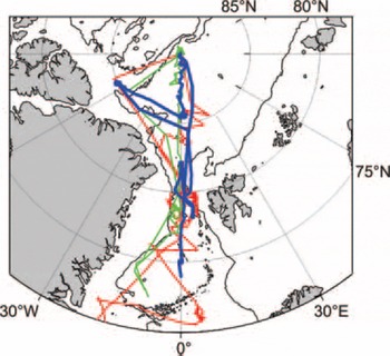
figure 1 shows schematically the track of the submarine and those of previous cruises in the areas of interest. the track within the eurasian basin north of fram strait consisted of northbound and southbound at 5˚ e with an excursion to the european commission greenice project ice-camp area at 62˚w along the 85˚n line of latitude. the areas of interest for our analysis were an area around 82˚n on the greenwich meridian which was covered by coincident envisat asar scene acquisitions and the 85˚n leg where Tireless transited sea-ice shear zones north of greenland.
Fig. 1. Submarine tracks: 1976 (red), 1987 (green) and 2004 (blue). The 2000m isobath is also shown as a thin solid line.
Oceanographic data analysis for this paper is expanded from that which was conducted on board Tireless to cover periods when personnel were off duty and the resultant gaps in the observer logs.
Fram Strait
A region on the greenwich meridian at 82˚n was chosen for daily envisat asar narrow swath scene acquisition during the period of the submarine voyage, with the aim of acquiring a scene coincident with the submarine upward-looking sonar and sidescan. this was achieved for scenes on 1, 4, 5 and 7 april as the submarine manoeuvred in and out of the miz prior to commencing deep penetration of the arctic ice pack. the area is in the main transpolar drift stream of ice advecting out of the arctic and so consists of concentrated but broken floes of mixed ages. data from this area can be used in studying sea-ice dynamics and the effects of melting on the ice canopy.
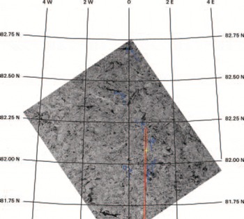
figure 2 shows an envisat scene acquired at 19:47:34 utc on 1 april coincident with the submarine track. backscatter intensity values were extracted from this image along the submarine track using erdas imagine software. a limited section of sea-ice draft was extracted from the relevant 780 chart roll for 10 km on both sides of the image acquisition time. previous studies by Reference Comiso, Wadhams, Krabill, Swift, Crawford and TuckerComiso and others (1991) and wadhams and others (1991) have found that a moderate positive correlation (0.68) exists. however, these studies used a single dataset where the synthetic aperture radar (sar) was an airborne x-band system, rather than the c-band carried by satellites. attempts to verify these results using the Trafalgar 1996 and first-generation satellite synthetic aperture radar (european remote-sensing satellite-2) were inconclusive (Reference Doble, Wadhams, Tuhkuri and RiskaDoble and wadhams, 1999).
Fig. 2. Coincident single polarity Envisat ASAR scene acquired at 19:47:34 UTC on 1 April 2004. The submarine track is marked in red, with position at time of image acquisition marked by a yellow cross-hair. Averaged drift of ice features over 12 hours before and after the time of image acquisition are marked with the blue arrows (to scale). Converted to velocities, for points A and B this was 0.22 ms–1 followed by 0.11 ms–1. For points C–F, drift was 0.19 ms–1 followed by 0.082 ms–1. Position of the tracked feature at the time of acquisition is shown by a blue circle.
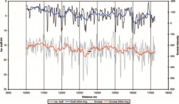
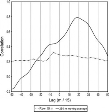
A comparison of the raw ice draft with the image intensity values from envisat does not show any clear correlation (fig. 3). however, by calculating a moving average of both the draft and intensity profiles it is possible to remove most of the variability and use the underlying trends to improve the correlation. an averaging length of 252mhas been suggested as optimal (wadhams and others, 1991). marking of time points on the paper chart rolls, and hence position along track, depend on the diligence of the 780 operator who has to decide when to press the appropriate button on the recorder. therefore a plot of cross-correlation (fig. 4) of a 5 km long section at lags between ±750m was produced which as the submarine was travelling at 2.2 knots (1.13ms–1) equates to ±11 min. the peak correlation (r) of the raw 15 m resolution data was 0.32 at a lag of –90 m. on applying the moving average of 250m the correlation peaks at 0.79 at a lag of +270 m. these are equivalent to 80 and 238 s in time.

Fig. 3. Envisat ASAR image intensity values vs ice draft from 1 April scene pixels.

Fig. 4. Cross-correlation between ice draft and Envisat image intensity. The raw 15 m resolution data show very little correlation. Application of a 250 m moving average produces a high correlation of 0.79 at a lag of +270 m.
One of the reasons why it is very difficult to synchronize the ice draft with the envisat scene is that the upward-looking echo-sounder profile gives no clues as to ridge orientation. the area covered by envisat for this study was a homogeneous mix of first- and multi-year floes, with numerous leads and ridging, typical of this area in spring. this provides no large open-water or rubble field areas which can be used to match the timing of the two profiles. in this type of environment, sidescan or multibeam imagery of the ice underside is essential for correctly identifying features.
An additional problem with linking the two data sources is that the submarine was moving very slowly at 1.13 ms–1. in regions like the transpolar drift, where ice has been observed to move at 10 kmd–1 (0.12ms–1), this can lead to a significant difference to the actual speed relative to the ice. to determine whether this factor was affecting the ice-draft data, two additional envisat alternating polarity (hh/hv) scenes at 18:38:58 utc on 31 march and 12:37:05 utc on 2 april were processed. distinct ice features were identified and their tracks recorded. based on these data, vectors of average ice drift for the 12 hours before and 12 hours after the envisat scene acquisition are also shown in figure 2. although the timing resolution is coarse, the results reveal that the ice drift was atypical of the area. in the 25 hours between the 31 march and 1 april scenes, ice drift was north-northwest at an average of 0.19ms–1. for the 17 hours between scenes on 1 and 2 april, ice drift reversed to southeast at 0.082 ms–1. ice north of 82˚15' n moved faster at 0.22 and 0.11 ms–1 for these periods. this resulted in the development of east–west leads. as Tireless was travelling north before scene acquisition and south after, this suggests that the ice-draft profile length scale will be compressed and elongated respectively. as a result, the cross-correlation of the 250 m moving averaged data series drops off away from the time of the envisat scene acquisition.
The results from the analysis of ice-draft data and coincident envisat scenes at 82˚n show that it is extremely difficult to match ice-draft data with c-band sar when the ice-draft data consist solely of a profile with no sidescan images port and starboard of the submarine track to allow positive feature recognition. key factors identified as needing further study include accurate measurement of the submarine’s speed against that of the ice above and knowledge of ice-drift patterns at and around the time of sar scene acquisition. despite this, the analysis has shown that it is possible to co-locate features in sar images and ice-draft profiles as long as good positional data are available.
85˚N Latitude
After working in fram strait, Tireless headed for the site of the later (may 2004) greenice ice-camp site at 85˚ n, 62˚ w. ice thickness was measured en route, along with oceanographic and bathymetric surveying. profiles were limited to uissxbt (under ice submarine expendable bathythermo-graph) probes, which only measure a temperature profile, as the uissxsvs (expendable sound velocimeters) available were found to be unreliable. despite this setback, it was possible to investigate oceanographic conditions seen by previous fieldwork in the region by scicex and surface ships in the 1990s (Reference Steele and BoydSteele and boyd, 1998), in particular the erosion of the arctic cold halocline layer (chl) by incursion of atlantic water (aw) into the arctic basin as evidenced by water warmer than the 0˚c isotherm.
Profiling was conducted using the available uissxbts and supplemented by the on-board oceanographic sensor suite by diving the submarine from minimum to maximum operating depth. successful uissxbts were launched at 10, 20, 30, 40, 50 and 60˚w, and Tireless conducted depth excursions at 5, 25, 35, 45 and 55˚ w.
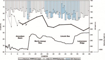
figure 5 shows an east–west profile along 85˚n showing parameters measured. sea-ice thickness increased heading west into what is traditionally seen as a zone of ice shearing between the beaufort gyre ice and the transpolar drift. the depth of the 0˚c isotherm also increased with the exception of a region between 10 and 30˚w. this is believed to be an area where pacific water follows the morris jessup rise protrusion of the greenland continental shelf around from the canada basin.
Fig. 5. East–west profile along 85˚N showing maximum keel depth, depth of the 0˚C isotherm (Atlantic Water) and bathymetry from the observation log of Tireless. Previous measurements along this line are also shown including maximum keel depths from Superb 1987, and depth of 0˚C isotherm from Oden 1991.
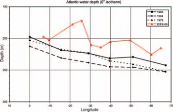
The environmental working group (ewg) atlas (timo-khov and tanis, 1997) is a compilation of russian and western winter hydrographic data taken from 1948 to 1987. in figure 6 a comparison of the ewg climatology with the data collected by Tireless shows a decrease in the cold-water-layer thickness of around 10–15 m. conductivity–temperature–depth (ctd) profiles collected by the swedish icebreaker Oden in 1991 (source: java ocean atlas, http://odf.ucsd.edu/joa/jsindex.html) overlap the eastern part of the Tireless section. no significant difference in aw depth is evident in the overlapping section, and the Oden data show the initial upslope of an apparent decrease in the cold-water-layer thickness at its western end, which would agree with the results from Tireless. the decrease in the cold-water-layer thickness continues up to 30˚w, from where the slope of increasing thickness of the cold water layer is resumed. an examination of the underlying bathymetry suggests a relationship with the morris jessup rise that may be generating a large-scale flow disturbance. the cold water layer increased in thickness heading west through the lincoln sea and onto the southern end of the lomonosov ridge.
Fig. 6. Depth of the 0˚C isotherm measured by Tireless compared with data from the EWG climatology (Reference Timokhov and TanisTimokhov and Tanis, 1997) showing decrease in thickness of the surface water layer.
Sea-ice draft values appeared to be consistent with Superb 1987 until 45˚w. to the west of this point, in the region also covered by the greenice ice-camp fieldwork, maximum keel depths were greater than observed in 1987. figure 5 shows mean maximum draft values (in 18 longitude bins) for the transect from the observer logs for the 780-type sonar. this has a wider beam angle which truncates the tips of keels, and the maximum keel depth measured was 32 m. the same keel measured using the narrow beam 2077-type sonar peaked at 34.4 m. keel depths were seen to approach and occasionally exceed the maxima observed by Superb (Reference WadhamsWadhams, 1990) along the length of the transect but not those of Sovereign 11 years earlier where there were 45 ridges exceeding 30m and the deepest exceeded 45 m (Reference Wadhams and N.Wadhams, 1986). the Superb and Tireless voyages both took place in april. Sovereign transited the area in october and it would be expected that in late summer ice drafts would be reduced. winter conditions observed in 2004 may be approaching those of 1987 but are still well short of summer conditions in 1976. these tentative results clearly point to the need for full analysis of the dataset and, to be consistent, a revised analysis of the earlier datasets using modern computer processing techniques.
Conclusion
Whilst sea ice in the arctic is observed to be decreasing in extent and thickness, there would still appear to be regions where large-scale ice circulation patterns are maintaining a population of ridge keels similar to that observed in the 1980s. in the late 1990s it was believed that the beaufort gyre had weakened, reducing ice thicknesses north of greenland. the situation almost 10 years later suggests that a late-1980s circulation regime has re-established itself. more work monitoring ice thicknesses and ridge development in this area of the arctic is still required. however, the nature of the ice limits access to aircraft and underwater vehicles.
With regard to the decrease in the chl, the oceanographic data collected by Tireless should be valuable for the study of the data-sparse morris jessup rise area. a decrease in the cold-water-layer thickness, compared to the existing ewg climatology (Reference Timokhov and TanisTimokhov and tanis, 1997), was observed in the area north of greenland. this, though, is probably due to a lack of data used to generate the climatology grids.
Tireless was also in the right location to provide sea-ice thickness measurements to validate algorithms using envisat asar data. our initial study shows that it is possible to synchronize the older type of paper echo-sounder record used with image intensity. further work to see whether parameters of ridges observed by the satellite can be quantified and then validated using the submarine sonar records is awaiting processing of the digital echo-sounder and sidescan records.
The icex-04 demonstrates that manned submarines still have a role to play in scientific exploration of the arctic ocean. whilst most autonomous underwater vehicle (auv) technology has advanced, the battery technology to power them has not, thus limiting the range over which they can operate. the use of a full-size submarine provides scope for pan-arctic monitoring and a flexibility to reverse course and carry out a detailed survey of an area of interest as it is encountered.
With the upcoming international polar year (ipy) in 2007–08, it is hoped that manned submarines will play a role in data gathering in the arctic ocean. this will very much depend on the objectives of the navies operating these vehicles. the last international geophysical year in 1957–58 was important for submarine exploration of the arctic and it is hoped that studies on that scale will be repeated in the ipy.
Acknowledgements
We are grateful to the uk ministry of defence (navy) for the release of data and for the opportunity to take part in the voyages concerned; and to the commanding officer and crew of hms Tireless for making so much of the scientific plan possible. we also thank the european commission project evk3-ct-2002-00083 ‘ice ridging information for decision making in shipping operations’ (iris) for funding the travel costs for embarkation and disembarkation and production and presentation of this paper. the envisat scenes used in this analysis were provided courtesy of european space agency (esa) envisat announcement of opportunity project no. 208.