


1. Introduction
Many natural and industrial processes involve the flow of solid particles, liquid droplets or gaseous bubbles whose dynamical evolution and morphology are intimately coupled with a carrier fluid. A peculiar behaviour of disperse multiphase flows is their ability to give rise to large-scale structures (hundreds to thousands of times the size of individual particles), from dense clusters to nearly particle-free voids (see figure 1). The emergence of spatial segregation in particles can be attributed to a number of factors, e.g. due to dissipation during inelastic collisions (Hopkins & Louge Reference Hopkins and Louge1991; Goldhirsch & Zanetti Reference Goldhirsch and Zanetti1993), viscous damping by the fluid (Wylie & Koch Reference Wylie and Koch2000), preferential concentration of particles by the background turbulence (Eaton & Fessler Reference Eaton and Fessler1994) and instabilities that arise due to interphase coupling (Glasser, Sundaresan & Kevrekidis Reference Glasser, Sundaresan and Kevrekidis1998; Agrawal et al. Reference Agrawal, Loezos, Syamlal and Sundaresan2001; Capecelatro, Desjardins & Fox Reference Capecelatro, Desjardins and Fox2014, Reference Capecelatro, Desjardins and Fox2015). Such large-scale heterogeneity can effectively ‘demix’ the underlying flow, reducing contact between the phases and resulting in enormous consequences at scales much larger than the size of individual particles, such as hindered heat and mass transfer (Agrawal et al. Reference Agrawal, Holloway, Milioli, Milioli and Sundaresan2013; Miller et al. Reference Miller2014; Pouransari & Mani Reference Pouransari and Mani2017; Beetham & Capecelatro Reference Beetham and Capecelatro2019; Guo & Capecelatro Reference Guo and Capecelatro2019).

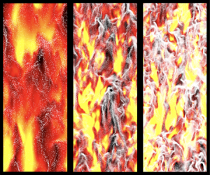
Figure 1. Instantaneous snapshots of fully developed CIT at statistical steady state. A slice at the centreline in the  $x$–
$x$– $y$ plane is shown, with particle position (white) and normalized vertical fluid velocity
  $u_f/\mathcal {V}_0$ (colour): (a)
  $Ar = 1.80$; (b)
  $Ar = 5.40$; and (c)
  $Ar = 18.0$.
The focus of the present work is on modelling disperse multiphase turbulence at length scales much larger than the particle diameter. Such flows can be categorized into two broad classes: (i) flows where the turbulence originates in the continuous phase with the discrete phase modulating the small scales of the turbulence (see e.g. Balachandar & Eaton (Reference Balachandar and Eaton2010), and references therein); and (ii) flows where the turbulence arises due to the coupling between the discrete and continuous phases. The former is mainly focused on how the discrete phase modifies the classical turbulence structures seen in single-phase flows. The latter is the focus of the present work and can be observed in gas–particle flows when the mass of the particles is of the same order or greater than that of the gas phase, or in bubbly flows when the bubble volume fraction is high enough to lead to buoyancy-driven instabilities (e.g. Besnard, Harlow & Rauenzhan Reference Besnard, Harlow and Rauenzhan1987; Rzehak & Krepper Reference Rzehak and Krepper2013; Ma, Lucas & Bragg Reference Ma, Lucas and Bragg2020).
To date, turbulent particle-laden flows are most often discussed in the dilute limit where the fluid-phase turbulence interacts with inertial particles without significant feedback from the particles. It is well established that dilute suspensions of heavy particles in isotropic turbulence will preferentially concentrate in regions of high strain rate and low vorticity (Eaton & Fessler Reference Eaton and Fessler1994). In the presence of a mean body force (e.g. gravity), particles have been observed to experience enhanced settling as a result of preferential sweeping, by which the particles tend toward regions of downward fluid motion when encountering vortical structures in the flow (e.g. Wang & Maxey Reference Wang and Maxey1993; Aliseda et al. Reference Aliseda, Cartellier, Hainaux and Lasheras2002; Ferrante & Elghobashi Reference Ferrante and Elghobashi2003; Yang & Shy Reference Yang and Shy2003; Bosse, Kleiser & Meiburg Reference Bosse, Kleiser and Meiburg2006).
When the particle concentration is sufficiently high, the background flow is largely controlled by interphase coupling. Under these conditions, particles tend to accumulate in regions of low vorticity, resembling preferential concentration that typically occurs in dilute particle-laden turbulence. However, in the dense limit the vorticity is generated in shear layers between highly concentration regions (clusters), unlike in classical preferential concentration where vorticity would exist even in the absence of the disperse phase (Capecelatro et al. Reference Capecelatro, Desjardins and Fox2015). Additional effects contribute to the settling velocity and spatial segregation of particles in denser suspensions when two-way coupling between the phases is non-negligible.
Seminal works by G. K. Batchelor have provided theoretical estimates describing the motion of collections of solid particles suspended in viscous flows (Batchelor Reference Batchelor1972, Reference Batchelor1982), in addition to important insights into the instabilities present in such systems. For example, Batchelor (Reference Batchelor1988) demonstrated that small rigid spheres falling under gravity will give rise to long-range hydrodynamic interactions that result in hindered settling (Batchelor Reference Batchelor1972). In more recent studies, it was demonstrated that, at higher Reynolds numbers and particle concentrations, momentum exchange between the phases results in enhanced settling when the mean mass loading,  $\varphi$, defined by the ratio of the specific masses of the particle and fluid phases, is of order one or larger (Capecelatro et al. Reference Capecelatro, Desjardins and Fox2015). In statistically homogeneous gravity-driven gas–solid flows, the average particle settling speed,
  $\mathcal {V}$, can be approximated as
 \begin{equation} \mathcal{V} = \mathcal{V}_0 + \langle u_f \rangle_p \end{equation}
for Stokes flow (Capecelatro et al. Reference Capecelatro, Desjardins and Fox2015), where  $\mathcal {V}_0=\tau _p g$ is the terminal Stokes settling velocity of an isolated particle with
  $\tau _p$ the particle response time and
  $g$ gravity. In this expression, the phase-averaged fluid velocity,
 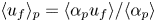 $\langle u_f \rangle _p = \langle \alpha _p u_f \rangle / \langle \alpha _p \rangle$, is sometimes referred to as the velocity seen by the particles, where
  $u_f$ is the local fluid velocity aligned with gravity,
  $\alpha _p$ is the local particle volume fraction and angled brackets denote a spatial and temporal average. At sufficient mass loading, fluctuations in particle concentration can generate and sustain fluid-phase turbulence (as shown in figure 1), referred to here as cluster-induced turbulence (CIT). Because clusters entrain the carrier phase,
  $u_f$ and
  $\alpha _p$ are often highly correlated, resulting in
  $\mathcal {V}>\mathcal {V}_0$.
Due to the breadth of length and time scales present in turbulent fluid–particle mixtures, accurate modelling of industrial and environmental flows remains challenging. Thus, the Reynolds-averaged Navier–Stokes (RANS) equations are the workhorse of industry to inform engineering designs and decisions. Because of the importance of the multiphase physics present in large-scale systems, developing multiphase RANS closures that are accurate under relevant conditions is critically important.
To date, multiphase turbulence models have largely relied upon extensions to single-phase models (e.g. Sinclair & Jackson Reference Sinclair and Jackson1989; Dasgupta, Jackson & Sundaresan Reference Dasgupta, Jackson and Sundaresan1994; Sundaram & Collins Reference Sundaram and Collins1994; Cao & Ahmadi Reference Cao and Ahmadi1995; Dasgupta, Jackson & Sundaresan Reference Dasgupta, Jackson and Sundaresan1998; Cheng et al. Reference Cheng, Guo, Wei, Jin and Lin1999; Zeng & Zhou Reference Zeng and Zhou2006; Jiang & Zhang Reference Jiang and Zhang2012; Rao et al. Reference Rao, Curtis, Hancock and Wassgren2012) that were derived directly from the Navier–Stokes equations. It should be noted, however, that multiphase turbulence does share some commonalities with single-phase flows, especially with variable-density turbulence. For example, multiphase flows subject to mean shear can develop velocity fluctuations that strongly modify the mean velocity profiles and transport properties of the flow (Capecelatro, Desjardins & Fox Reference Capecelatro, Desjardins and Fox2018). Single-phase, variable-density flows subject to Rayleigh–Taylor instabilities (see, e.g. Johnson & Schilling Reference Johnson and Schilling2011; Zhou Reference Zhou2017) develop velocity and density fluctuations similar to those observed in heterogeneous bubbly flows (Mudde Reference Mudde2005). However, the main difference between disperse multiphase and variable-density flows is that the former has a separate velocity for each phase while the latter has a single fluid velocity. Moreover, momentum coupling by particles introduces velocity fluctuations at small scales that further complicates the energy budget of turbulence. By introducing the slip velocity, i.e. the velocity difference between the discrete and continuous phases, additional dimensionless parameters, such as the Stokes number and mass loading, are needed to describe multiphase turbulence.
In contrast to modelling by analogy with single-phase flow, Fox (Reference Fox2014) developed the exact Reynolds-averaged equations for collisional fluid–particle flows. In that work, it was demonstrated that directly averaging the Navier–Stokes equations fails to capture important two-phase interactions. Instead, it was demonstrated that phase averaging the mesoscale (locally averaged) equations results in a set of equations that explicitly account for two-way coupling contributions. Capecelatro et al. (Reference Capecelatro, Desjardins and Fox2015) further developed the Reynolds-averaged formulation of Fox (Reference Fox2014) to include transport equations for the volume-fraction variance, drift velocity and the separate components of the Reynolds stresses of each phase and particle-phase pressure tensor. While exact, it does lead to a large number of unclosed terms that require modelling, which is the focus of the present study.
Accurate modelling of the unclosed terms that remain predictive from dilute to dense regimes remains an outstanding challenge. Fox (Reference Fox2014) proposed closures of the phase-averaged (PA) terms based largely on single-phase turbulence models without extensive validation. Capecelatro, Desjardins & Fox (Reference Capecelatro, Desjardins and Fox2016b) extended these models to account for near-wall effects in particle-laden channel flows. Agreement with the turbulence statistics obtained from simulation data was found to be satisfactory at first order (e.g. PA velocities) but less so at second order (e.g. PA turbulent kinetic energy). Innocenti et al. (Reference Innocenti, Fox, Salvetti and Chibbaro2019) drew upon a probability-density-function approach, along with extensions from single-phase turbulence modelling (particularly in the fluid phase), showing satisfactory agreement for statistics up to second order. However, the model was restricted to relatively dilute flows. Due to the large parameter space associated with turbulent multiphase flows, a reliable modelling approach valid across two-phase flow regimes (e.g. dilute to dense limit) remains elusive.
Broadly speaking, extracting new models and understanding of physics from data has a long history in many diverse areas of science and engineering (see e.g. Jordan & Mitchell Reference Jordan and Mitchell2015). In the last decade, these data-driven techniques have been applied to turbulence modelling in several ways, including uncertainty prediction and quantification, model calibration and augmentation and the generation of entirely new models. Several recent works have utilized machine learning (neural networks are particularly popular; Milano & Koumoutsakos Reference Milano and Koumoutsakos2002; Lu Reference Lu2010; Rajabi & Kavianpour Reference Rajabi and Kavianpour2012; Duraisamy & Durbin Reference Duraisamy and Durbin2014; Duraisamy, Zhang & Singh Reference Duraisamy, Zhang and Singh2015; Tracey, Duraisamy & Alonso Reference Tracey, Duraisamy and Alonso2015; Ling, Kurzawski & Templeton Reference Ling, Kurzawski and Templeton2016; Ma, Lu & Tryggvason Reference Ma, Lu and Tryggvason2016; Bode et al. Reference Bode, Gauding, Kleinheinz and Pitsch2019; Liu & Fang Reference Liu and Fang2019) in order to translate large amounts of experimental or computational data into model closures. Neural networks have shown relatively exceptional performance outside the region in which they were trained. As a departure from more traditional modelling techniques, these methods are inserted modularly, as a ‘black box’, into an existing flow solver. Thus, while they have displayed a high level of performance on a wide range of flow conditions, the closure does not satisfy the interpretability condition necessary for making physical inferences. Further, a large number of neural network approaches attempt to augment or correct existing models. However, as discussed above, in the context of multiphase flows appropriate existing models in which to augment do not exist.
Rather than relying on a best-fit strategy, as done in neural networks, Brunton, Proctor & Kutz (Reference Brunton, Proctor and Kutz2016) developed a strategy based on sparse regression that identifies the underlying functional form of the nonlinear physics by optimizing a coefficient matrix that acts upon a matrix of trial functions. While this method requires knowledge about the physics of the system under configuration (in order to make informed selections of the trial functions), it can be reasonably assumed that the modeller is not entirely naive. In fact, traditional modelling techniques have relied nearly exclusively on this notion. Schmelzer, Dwight & Cinnella (Reference Schmelzer, Dwight and Cinnella2020) and Beetham & Capecelatro (Reference Beetham and Capecelatro2020) recently extended the sparse identification framework of Brunton et al. (Reference Brunton, Proctor and Kutz2016) to infer algebraic stress models for the closure of RANS equations. In Schmelzer et al. (Reference Schmelzer, Dwight and Cinnella2020) the models are written as tensor polynomials and built from a library of candidate functions. In Beetham & Capecelatro (Reference Beetham and Capecelatro2020) Galilean invariance of the resulting models are guaranteed through thoughtful tailoring of the feature space.
In this work, the sparse identification modelling framework of Beetham & Capecelatro (Reference Beetham and Capecelatro2020) is employed to develop multiphase closure models for homogeneous, gravity-driven gas–solid flows. Eulerian–Lagrangian simulations are performed across a range of Archimedes numbers and volume fractions to provide training data. The terms appearing in the multiphase RANS equations recently derived in Capecelatro et al. (Reference Capecelatro, Desjardins and Fox2015) are extracted. We then build a minimally invariant basis set of tensors (i.e. a set of functional groups that serve as candidate terms in the desired model). Such basis sets are well established for single-phase turbulent flows (Pope Reference Pope1975; Speziale, Sarkar & Gatski Reference Speziale, Sarkar and Gatski1991; Gatski & Speziale Reference Gatski and Speziale1993); however, an analogous basis has not yet been determined for multiphase flows. Using this basis and the sparse regression methodology, the compact functional form of the physics-based closures are inferred. As we consider exclusively statistically stationary and homogeneous systems, model realizability (Pope Reference Pope2000) is left for future work.
2. System description
2.1. Configuration under study
In the present study, rigid spherical particles of diameter  $d_p$ and density
  $\rho _p$ are suspended in an unbounded (triply periodic) domain containing an initially quiescent gas of density
  $\rho _f$ and viscosity
  $\nu _f$. Gravity
  $g$ acts in the negative
  $x$-direction. As particles settle, they spontaneously form clusters. Due to two-way coupling between phases, particles entrain the fluid, generating turbulence therein. A frame of reference with the fluid phase is considered, such that the mean streamwise fluid velocity is null. Given the relative simplicity of the configuration, only a few non-dimensional groups arise. An important non-dimensional number is the Archimedes number, defined as
 \begin{equation} {\textit{Ar}} = (\rho_p/\rho_f -1)d_p^3 g/\nu_f^2. \end{equation}
Alternatively, a Froude number can be introduced to characterize the balance between gravitational and inertial forces, defined as  ${\textit {Fr}}= \tau _p^2 g/ d_p$, where
  $\tau _p = {\rho _p d_p^2}/{(18 \rho _f \nu _f)}$ is the particle response time. The Stokes settling velocity for an isolated particle is given by
  $\mathcal {V}_0=\tau _p g$. From this a characteristic cluster length can also be estimated a priori as
  $\mathcal {L} = \tau _p^2 g$. To ensure the hydrodynamics is independent of the domain size, the simulation configurations are equal or larger than Case 4 reported in Capecelatro, Desjardins & Fox (Reference Capecelatro, Desjardins and Fox2016a).
To sample the parameter space typical of turbulent fluidized bed reactors (Sun & Zhu Reference Sun and Zhu2019), the mean particle-phase volume fraction is varied in the range  $0.001\le \langle \alpha _p\rangle \le 0.05$ and the Archimedes number is varied in the range
  $1.8\le {\textit {Ar}}\le 18.0$ by adjusting gravity. Due to the large density ratios under consideration, the mean mass loading ranges from
  ${O}(10)$ to
  ${O}(10^2)$, and consequently two-way coupling between the phases is expected to be important. Here, angled brackets denote both a spatial and a temporal average (since the flow under consideration is triply periodic and statistically stationary in time). A list of relevant non-dimensional numbers and other important simulation parameters are summarized in table 1.
Table 1. Summary of parameters for the configurations under consideration.

2.2. Volume-filtered equations
In this section, we present the volume-filtered Eulerian–Lagrangian equations used to formulate the Reynolds-averaged equations in § 3 and generate the simulation data that will be applied to the sparse regression methodology in § 4. The position and velocity of the  $i$th particle is calculated according to Newton's second law
 \begin{equation} \frac{\textrm{{d}}\kern0.06em \boldsymbol{x}_p^{(i)}}{\textrm{{d}}t} =\boldsymbol{v}_p^{(i)}\quad \textrm{{and}}\quad \frac{\textrm{{d}} \boldsymbol{v}_p^{(i)}}{\textrm{{d}}t} = \mathcal{A}^{(i)} + \boldsymbol{F}_c^{(i)} + \boldsymbol{g}, \end{equation}
where  $\boldsymbol {x}_p^{(i)}$ is the centre position of particle
  $i$ and
  $\boldsymbol {v}_p^{(i)}$ is its velocity at time
  $t$ and
  $\boldsymbol {g} = (-g,0,0)^{\textrm {{T}}}$ is the acceleration due to gravity. The force due to inter-particle collisions,
  $\boldsymbol {F}_c$, is accounted for using a soft-sphere collision model originally proposed by Cundall & Strack (Reference Cundall and Strack1979). Particles are treated as inelastic and frictional with a coefficient of restitution of
  $0.85$ and coefficient of friction of
  $0.1$ (Capecelatro & Desjardins Reference Capecelatro and Desjardins2013). Momentum exchange between the phases is given by
 \begin{equation} \mathcal{A}^{(i)} = \frac{ {F}_d }{\tau_p} \left(\boldsymbol{u}_f - \boldsymbol{v}_p^{(i)} \right)- \frac{1}{\rho_p} \boldsymbol{\nabla} p_f + \frac{1}{\rho_p} \boldsymbol{\nabla} \boldsymbol{\cdot} \boldsymbol{\sigma}_f, \end{equation}
where  $\boldsymbol {u}_f$,
  $p_f$ and
  $\boldsymbol {\sigma }_f$ are the fluid-phase velocity, pressure, and viscous-stress tensor evaluated at the particle location, respectively, and
  $F_d$ is the non-dimensional drag correction of Tenneti & Subramaniam (Reference Tenneti and Subramaniam2011) that takes into account local volume fraction and Reynolds number effects given by
 \begin{equation} F_d(\alpha_f,{\textit{Re}}_p)=\frac{1+0.15{Re}_p^{0.687}}{\alpha_f^2}+\alpha_f F_1 \left( \alpha_f \right)+\alpha_f F_2\left( \alpha_f,{Re}_p \right), \end{equation}
where the particle Reynolds number is defined as
 \begin{equation} {\textit{Re}}_p = \frac{ \alpha_f \vert \boldsymbol{u}_f - \boldsymbol{v}_p^{(i)} \vert d_p}{\nu_f}. \end{equation}
The remaining two terms in (2.4) are given by
 \begin{gather} F_1( \alpha_f )=\frac{5.81\alpha_p}{\alpha_f^3}+\frac{0.48\alpha_p^{1/3}}{\alpha_f^4}, \end{gather}
 \begin{gather}F_2( \alpha_f,{Re}_p )=\alpha_p^3{Re}_p\left(0.95+\frac{0.61\alpha_p^3}{\alpha_f^2}\right), \end{gather}
where  $\alpha _f=1-\alpha _p$ is the fluid-phase volume fraction.
To account for the presence of particles in the fluid phase without resolving the boundary layers around individual particles, a volume filter is applied to the incompressible Navier–Stokes equations (Anderson & Jackson Reference Anderson and Jackson1967). This procedure replaces the point variables with smooth, locally filtered fields. These volume-filtered equations are given by
 \begin{equation} \frac{\partial \alpha_f}{\partial t} + \boldsymbol{\nabla}\boldsymbol{\cdot} \left(\alpha_f \boldsymbol{u}_f\right) = 0 \end{equation}
and
 \begin{equation} \frac{\partial \alpha_f \boldsymbol{u}_f}{\partial t} + \boldsymbol{\nabla}\boldsymbol{\cdot} \left( \alpha_f \boldsymbol{u}_f \otimes \boldsymbol{u}_f \right) ={-}\frac{1}{\rho_f} \boldsymbol{\nabla} p_f +\boldsymbol{\nabla} \boldsymbol{\cdot} \boldsymbol{\sigma}_f - \frac{\rho_p}{\rho_f} \alpha_p \mathcal{A} + \alpha_f \boldsymbol{g}, \end{equation}
where  $\mathcal {A}$ is the locally averaged momentum exchange term, evaluated at each Lagrangian particle and projected to the Eulerian mesh. The fluid-phase viscous-stress tensor is defined as
 \begin{equation} \boldsymbol{\sigma}_{f} = \nu_f \left \lbrack \boldsymbol{\nabla} \boldsymbol{u}_f + \left(\boldsymbol{\nabla} \boldsymbol{u}_f \right)^{\textrm{{T}}} - \tfrac{2}{3} \boldsymbol{\nabla} \boldsymbol{\cdot} \boldsymbol{u}_f \boldsymbol{\mathbb{I}} \right \rbrack, \end{equation}
where  $\boldsymbol {\mathbb {I}}$ is the identity matrix.
The Eulerian–Lagrangian equations are solved using NGA (Desjardins et al. Reference Desjardins, Blanquart, Balarac and Pitsch2008), a fully conservative, low-Mach-number finite volume solver. A pressure Poisson equation is solved to enforce continuity via fast Fourier transforms in all three periodic directions. The fluid equations are solved on a staggered grid with second-order spatial accuracy and advanced in time with second-order accuracy using the semi-implicit Crank–Nicolson scheme of Pierce (Reference Pierce2001). Lagrangian particles are integrated using a second-order Runge–Kutta method. Fluid quantities appearing in (2.2a,b) are evaluated at the position of each particle via trilinear interpolation. Particle data are projected onto the Eulerian mesh using the two-step filtering process described in Capecelatro & Desjardins (Reference Capecelatro and Desjardins2013).
2.3. Eulerian–Lagrangian training data
The Eulerian–Lagrangian simulations were initialized with a random distribution of particles and run for approximately  $100 \tau _p$ until the flow reached a statistically stationary state. At this point, statistics are accumulated over
  $50 \tau _p$. Instantaneous snapshots of the streamwise fluid velocity and particle position of each case at steady state are shown in figure 1. It can immediately be seen that clusters of particles are generated and entrain the fluid downward. As a consequence of the frame of reference under consideration, the fluid flows upward in regions void of particles. Clusters are seen to become more distinct with increasing
  $\langle \alpha _p\rangle$. The effect of
  ${\textit {Ar}}$ on the flow field is less noticeable. As shown in table 2, the standard deviation in volume-fraction fluctuations
  $\langle {\alpha _p^\prime }^2\rangle ^{1/2}$ increases with increasing
  ${\textit {Ar}}$, with
  $\alpha _p^\prime =\alpha _p-\langle \alpha _p\rangle$, indicating enhanced clustering. Perhaps less obvious, the volume-fraction fluctuations normalized by
  $\langle \alpha _p\rangle$ are maximum for the intermediate volume-fraction case (
 $\langle \alpha _p\rangle =0.025$).
Table 2. Statistically stationary Euler–Lagrange (EL) quantities for all nine training cases.

Because turbulence in CIT is driven by two-way coupling with the particle phase, there exist few characteristic scales that can be calculated a priori. However, the Taylor Reynolds number  ${\textit {Re}}_{\lambda } = u_{rms} \lambda /\nu _f$ and the Stokes number
  ${\textit {St}}_{\eta } = \tau _p/\tau _{\eta }$, both of which must be computed a posteriori, provide insight on the resulting turbulence. Here,
  $u_{rms}$ is the average root-mean-square velocity,
  $\lambda = \sqrt {15 \nu _f/\varepsilon _f} u_{rms}$ is the Taylor micro-scale with
  $\varepsilon _f$ the viscous dissipation rate and
  $\tau _{\eta }=\sqrt {\nu _f/\varepsilon _f}$ the Kolmogorov time scale. The values of these quantities for all nine cases are reported in table 2. It can be seen that high volume fractions correspond to larger Stokes numbers and lower values of
  ${\textit {Re}}_{\lambda }$. Both
  ${\textit {St}}_\eta$ and
  ${\textit {Re}}_{\lambda }$ tend to increase when larger body forces are applied (i.e. larger
  ${\textit {Ar}}$). Because fluid velocity fluctuations are generated by two-way coupling,
  ${\textit {Re}}_{\lambda }>0$ only when
  $\langle \alpha _p\rangle >0$. That said,
  ${\textit {Re}}_{\lambda }$ is seen to decrease with increasing
  $\langle \alpha _p\rangle$ for
  ${\textit {Ar}}=1.8$ and
  $5.4$. This is likely due to increased dissipation through drag exchange (see table 3). However, this reduction is less dramatic as
  ${\textit {Ar}}$ increases, and
  ${\textit {Re}}_{\lambda }$ is seen to be approximately constant at
  ${\textit {Ar}}=18$.

3. PA equations
In this section, we present the PA flow equations in which we seek to model the unclosed terms that arise. This system of equations has been previously derived (Capecelatro et al. Reference Capecelatro, Desjardins and Fox2015) and is extended here to take into account nonlinear drag effects due to  $F_d$ in (2.3).
The PA is analogous to Favre averaging of variable-density flows and is denoted by  $\langle (\cdot ) \rangle _p = \langle \alpha _p (\cdot ) \rangle /\langle \alpha _p \rangle$. Fluctuations about the PA particle velocity are expressed as
  $\boldsymbol {u}_p^{\prime \prime } = \boldsymbol {u}_p(\boldsymbol {x},t) - \langle \boldsymbol {u}_p \rangle _p$, with
  $\langle \boldsymbol {u}_p^{ \prime \prime } \rangle _p = 0$. This gives rise to the PA particle-phase turbulent kinetic energy (TKE),
  $k_p = \langle \boldsymbol {u}_p^{\prime \prime } \boldsymbol {\cdot} \boldsymbol {u}_p^{\prime \prime } \rangle _p/2$. Here,
  $\boldsymbol {u}_p$ is the particle-phase velocity in an Eulerian frame of reference. It should be noted that
  $\langle \boldsymbol {u}_p\rangle _p$ is equivalent to the average particle velocity
  $\langle \boldsymbol {v}_p\rangle$ (with angled brackets here used to represent a particle average). Thus,
  $\langle u_p\rangle _p$ will be used throughout to characterize the mean settling velocity of the particle phase. In a similar fashion, the PA operator in the fluid phase is defined as
  $\langle (\cdot ) \rangle _f = \langle \alpha _f (\cdot ) \rangle /\langle \alpha _f \rangle$. Fluctuations about the PA fluid velocity are given by
  $\boldsymbol {u}_f^{\prime \prime \prime } = \boldsymbol {u}_f(\boldsymbol {x},t) - \langle \boldsymbol {u}_f \rangle _f$. With this, the fluid-phase TKE is given by
  $k_f = \langle \boldsymbol {u}_f^{\prime \prime \prime } \boldsymbol {\cdot} \boldsymbol {u}_f^{\prime \prime \prime } \rangle _f/2$.
For the statistically stationary and homogeneous flows considered herein, continuity implies  $\langle \alpha _f\rangle$ is constant and the fluid-phase momentum equation reduces to
  $\langle \boldsymbol {u}_f\rangle _f=0$. In the particle phase, the only non-zero component of the averaged momentum equation is in the gravity-aligned direction (the
  $x$-direction in this case)
 \begin{equation} \frac{\partial \langle u_p \rangle_p}{\partial t} = \frac{1}{\tau_p^{{\star}}} \left( \langle u_f \rangle_p - \langle u_p\rangle_p \right) + \frac{1}{\rho_p} \left( \left \langle \frac{\partial \sigma_{f,xi}}{\partial x_i} \right \rangle_p - \left \langle \frac{\partial p_f}{\partial x} \right \rangle_p \right) + g, \end{equation}
noting that for gas–solid flows, the terms involving  $\sigma _{f,xi}$ and
  $p_f$ are small enough to be neglected (Capecelatro et al. Reference Capecelatro, Desjardins and Fox2015). This implies that at steady state,
  $\langle u_p\rangle _p \approx \langle u_f \rangle _p + \tau _p^{\star } g$. Here, we incorporate the nonlinearities associated with drag in
  $\tau _p^{\star } = \tau _p/\langle F_d \rangle _p$, where
  $\langle F_d \rangle _p(\langle \alpha _f\rangle ,\langle {\textit {Re}}_p\rangle )$ is the nonlinear drag correction (2.4) defined using averaged flow arguments. This definition does not include the dependencies on drag covariance terms (i.e.
  $\langle u_f^{\prime \prime \prime } F_d^{\prime \prime }\rangle _p$ and
  $\langle u_p^{\prime \prime } F_d^{\prime \prime }\rangle _p$), however, as shown in table 2, these terms have negligible contributions when describing particle settling,
  $\langle u_p \rangle _p$, and are thus neglected.
The transport equations for the fluid-phase Reynolds stresses can be reduced to two unique, non-zero components. In the streamwise direction this equation is given as
 \begin{align} \frac{1}{2} \frac{\partial
\langle u_f^{\prime \prime \prime 2}\rangle_f}{\partial t }
&= \underbrace{\frac{1}{\rho_f} \left \langle p_f
\frac{\partial u_f^{\prime \prime \prime} }{\partial
x}\right \rangle }_{{\scriptsize{pressure \ strain
(PS)}}} - \underbrace{\frac{1}{\rho_f} \left \langle
\sigma_{f,1i} \frac{\partial u_f^{\prime \prime \prime}
}{\partial x_i}\right \rangle }_{{\scriptsize{viscous \
dissipation (VD)}}} + \underbrace{
\frac{\varphi}{\tau_p^{{\star}}}\left( \langle u_f^{\prime
\prime \prime} u_p^{\prime\prime} \rangle_p - \langle
u_f^{\prime \prime \prime 2}\rangle_p
\right)}_{{\scriptsize{drag \ exchange (DE)}}}
\nonumber\\ &\quad
+\underbrace{\frac{\varphi}{\tau_p^{{\star}}} \langle
u_f^{\prime \prime \prime}\rangle_p \langle u_p\rangle_p
}_{{\scriptsize{drag \ production \ (DP)}}} +
\underbrace{\frac{\varphi}{\rho_p} \left \langle
u_f^{\prime\prime\prime}\frac{\partial
p^{\prime}_f}{\partial x} \right \rangle_p
}_{{\scriptsize{pressure \ exchange \ (PE)}}} -
\underbrace{\frac{\varphi}{\rho_p} \left \langle
u_f^{\prime \prime \prime} \frac{\partial
\sigma^{\prime}_{f,1i}}{\partial x_i} \right \rangle_p
}_{{\scriptsize{viscous \ exchange \ (VE)}}}.
\end{align}
\begin{align} \frac{1}{2} \frac{\partial
\langle u_f^{\prime \prime \prime 2}\rangle_f}{\partial t }
&= \underbrace{\frac{1}{\rho_f} \left \langle p_f
\frac{\partial u_f^{\prime \prime \prime} }{\partial
x}\right \rangle }_{{\scriptsize{pressure \ strain
(PS)}}} - \underbrace{\frac{1}{\rho_f} \left \langle
\sigma_{f,1i} \frac{\partial u_f^{\prime \prime \prime}
}{\partial x_i}\right \rangle }_{{\scriptsize{viscous \
dissipation (VD)}}} + \underbrace{
\frac{\varphi}{\tau_p^{{\star}}}\left( \langle u_f^{\prime
\prime \prime} u_p^{\prime\prime} \rangle_p - \langle
u_f^{\prime \prime \prime 2}\rangle_p
\right)}_{{\scriptsize{drag \ exchange (DE)}}}
\nonumber\\ &\quad
+\underbrace{\frac{\varphi}{\tau_p^{{\star}}} \langle
u_f^{\prime \prime \prime}\rangle_p \langle u_p\rangle_p
}_{{\scriptsize{drag \ production \ (DP)}}} +
\underbrace{\frac{\varphi}{\rho_p} \left \langle
u_f^{\prime\prime\prime}\frac{\partial
p^{\prime}_f}{\partial x} \right \rangle_p
}_{{\scriptsize{pressure \ exchange \ (PE)}}} -
\underbrace{\frac{\varphi}{\rho_p} \left \langle
u_f^{\prime \prime \prime} \frac{\partial
\sigma^{\prime}_{f,1i}}{\partial x_i} \right \rangle_p
}_{{\scriptsize{viscous \ exchange \ (VE)}}}.
\end{align}
Similarly, both cross-stream equations are given as
 \begin{align} \frac{1}{2} \frac{\partial
\langle v_f^{\prime \prime \prime 2}\rangle_f}{\partial t }
&= \underbrace{\frac{1}{\rho_f} \left \langle p_f
\frac{\partial v_f^{\prime \prime \prime}}{\partial
y}\right \rangle }_{{\scriptsize{PS}}} - \underbrace{\frac{1}{\rho_f} \left \langle
\sigma_{f,2i} \frac{\partial v_f^{\prime \prime
\prime}}{\partial x_i}\right \rangle
}_{{\scriptsize{VD}}} +
\underbrace{ \frac{\varphi}{\tau_p^{{\star}}}\left( \langle
v_f^{\prime \prime \prime} v_p^{\prime\prime} \rangle_p -
\langle v_f^{\prime \prime \prime 2}\rangle_p
\right)}_{{\scriptsize{DE}}}
\nonumber\\ &\quad +\underbrace{\frac{\varphi}{\rho_p}
\left \langle v_f^{\prime\prime\prime}\frac{\partial
p^{\prime}_f}{\partial y} \right \rangle_p
}_{{\scriptsize{PE}}} -
\underbrace{\frac{\varphi}{\rho_p} \left \langle
v_f^{\prime \prime \prime} \frac{\partial
\sigma^{\prime}_{f,2i}}{\partial x_i} \right \rangle_p
}_{{\scriptsize{VE}}},
\end{align}
\begin{align} \frac{1}{2} \frac{\partial
\langle v_f^{\prime \prime \prime 2}\rangle_f}{\partial t }
&= \underbrace{\frac{1}{\rho_f} \left \langle p_f
\frac{\partial v_f^{\prime \prime \prime}}{\partial
y}\right \rangle }_{{\scriptsize{PS}}} - \underbrace{\frac{1}{\rho_f} \left \langle
\sigma_{f,2i} \frac{\partial v_f^{\prime \prime
\prime}}{\partial x_i}\right \rangle
}_{{\scriptsize{VD}}} +
\underbrace{ \frac{\varphi}{\tau_p^{{\star}}}\left( \langle
v_f^{\prime \prime \prime} v_p^{\prime\prime} \rangle_p -
\langle v_f^{\prime \prime \prime 2}\rangle_p
\right)}_{{\scriptsize{DE}}}
\nonumber\\ &\quad +\underbrace{\frac{\varphi}{\rho_p}
\left \langle v_f^{\prime\prime\prime}\frac{\partial
p^{\prime}_f}{\partial y} \right \rangle_p
}_{{\scriptsize{PE}}} -
\underbrace{\frac{\varphi}{\rho_p} \left \langle
v_f^{\prime \prime \prime} \frac{\partial
\sigma^{\prime}_{f,2i}}{\partial x_i} \right \rangle_p
}_{{\scriptsize{VE}}},
\end{align}
where the drag production term no longer appears, since it is a gravity-driven phenomenon.
Due to the homogeneity of the flow and symmetry in the directions perpendicular to gravity ( $y$ and
  $z$ directions in this configuration), the unique, non-zero PA Reynolds-stress transport equations in the particle phase are given as
 \begin{align} \frac{1}{2} \frac{\partial
\langle u_p^{\prime \prime 2} \rangle_p}{\partial t} &=
\underbrace{\left \langle \varTheta \frac{\partial
u_p^{\prime \prime}}{\partial x} \right
\rangle_p}_{{\scriptsize{PS}}} -
\underbrace{\left \langle \sigma_{p,1i} \frac{\partial
u_p^{\prime \prime}}{\partial x_i} \right \rangle_p
}_{{\scriptsize{VD}}}+
\underbrace{\frac{1}{\tau_p^{{\star}}} \left( \langle
u_f^{\prime \prime \prime} u_p^{\prime \prime} \rangle_p -
\langle u_p^{\prime \prime 2}
\rangle_p\right)}_{{\scriptsize{DE}}}
\nonumber\\ &\quad\times \underbrace{\frac{1}{\rho_p}\left
\langle u_p^{\prime \prime} \frac{\partial
\sigma_{f,1i}^{\prime}}{\partial x_i} \right
\rangle_p}_{{\scriptsize{VE}}} -
\underbrace{\frac{1}{\rho_p} \left \langle u_p^{\prime
\prime} \frac{\partial p'_f}{\partial x}\right \rangle_p
}_{{\scriptsize{PE}}}.
\end{align}
\begin{align} \frac{1}{2} \frac{\partial
\langle u_p^{\prime \prime 2} \rangle_p}{\partial t} &=
\underbrace{\left \langle \varTheta \frac{\partial
u_p^{\prime \prime}}{\partial x} \right
\rangle_p}_{{\scriptsize{PS}}} -
\underbrace{\left \langle \sigma_{p,1i} \frac{\partial
u_p^{\prime \prime}}{\partial x_i} \right \rangle_p
}_{{\scriptsize{VD}}}+
\underbrace{\frac{1}{\tau_p^{{\star}}} \left( \langle
u_f^{\prime \prime \prime} u_p^{\prime \prime} \rangle_p -
\langle u_p^{\prime \prime 2}
\rangle_p\right)}_{{\scriptsize{DE}}}
\nonumber\\ &\quad\times \underbrace{\frac{1}{\rho_p}\left
\langle u_p^{\prime \prime} \frac{\partial
\sigma_{f,1i}^{\prime}}{\partial x_i} \right
\rangle_p}_{{\scriptsize{VE}}} -
\underbrace{\frac{1}{\rho_p} \left \langle u_p^{\prime
\prime} \frac{\partial p'_f}{\partial x}\right \rangle_p
}_{{\scriptsize{PE}}}.
\end{align}
Similarly, the cross-gravity equations are both (due to symmetry and homogeneity) given as
 \begin{align} \frac{1}{2} \frac{\partial
\langle v_p^{\prime \prime 2} \rangle_p}{\partial t} &=
\underbrace{\left \langle \varTheta \frac{\partial
v_p^{\prime \prime}}{\partial y} \right
\rangle_p}_{{\scriptsize{PS}}} -
\underbrace{\left \langle \sigma_{p,2i} \frac{\partial
v_p^{\prime \prime}}{\partial x_i} \right \rangle_p
}_{{\scriptsize{VD}}}+
\underbrace{\frac{1}{\tau_p^{{\star}}} \left( \langle
v_f^{\prime \prime \prime} v_p^{\prime \prime} \rangle_p -
\langle v_p^{\prime \prime 2}
\rangle_p\right)}_{{\scriptsize{DE}}}
\nonumber\\ &\quad\times \underbrace{\frac{1}{\rho_p}\left
\langle v_p^{\prime \prime} \frac{\partial
\sigma_{f,2i}^{\prime}}{\partial y_i} \right
\rangle_p}_{{\scriptsize{VE}}} -
\underbrace{\frac{1}{\rho_p} \left \langle v_p^{\prime
\prime} \frac{\partial p'_f}{\partial y}\right \rangle_p
}_{{\scriptsize{PE}}},
\end{align}
\begin{align} \frac{1}{2} \frac{\partial
\langle v_p^{\prime \prime 2} \rangle_p}{\partial t} &=
\underbrace{\left \langle \varTheta \frac{\partial
v_p^{\prime \prime}}{\partial y} \right
\rangle_p}_{{\scriptsize{PS}}} -
\underbrace{\left \langle \sigma_{p,2i} \frac{\partial
v_p^{\prime \prime}}{\partial x_i} \right \rangle_p
}_{{\scriptsize{VD}}}+
\underbrace{\frac{1}{\tau_p^{{\star}}} \left( \langle
v_f^{\prime \prime \prime} v_p^{\prime \prime} \rangle_p -
\langle v_p^{\prime \prime 2}
\rangle_p\right)}_{{\scriptsize{DE}}}
\nonumber\\ &\quad\times \underbrace{\frac{1}{\rho_p}\left
\langle v_p^{\prime \prime} \frac{\partial
\sigma_{f,2i}^{\prime}}{\partial y_i} \right
\rangle_p}_{{\scriptsize{VE}}} -
\underbrace{\frac{1}{\rho_p} \left \langle v_p^{\prime
\prime} \frac{\partial p'_f}{\partial y}\right \rangle_p
}_{{\scriptsize{PE}}},
\end{align}
where  $\varTheta$ and
  $\sigma _{p}$ are the granular temperature and the particle-phase viscous stress tensor, respectively (Capecelatro et al. Reference Capecelatro, Desjardins and Fox2015).
Due to the high density ratio in gas–solid flows, PE and VE are often negligible (Capecelatro et al. Reference Capecelatro, Desjardins and Fox2015). Therefore, the overall kinetic energy balance for CIT includes DP, PS, VD and DE. As in single-phase turbulence, VD results from the resolved small-scale velocity fluctuations in the fluid phase. In contrast, the drag exchange terms involve (i) DE $_2$: viscous dissipation of unresolved fluid velocity fluctuations (in the viscous boundary layers around individual particles) and (ii) DE
 $_1$: energy transferred to the particles at the fluid–particle interface. Sundaram & Collins (Reference Sundaram and Collins1999) showed that the unresolved dissipation arises in the point-particle model due to the difference between the fluid velocity at the particle location and the particle velocity. Our previous work (Capecelatro et al. Reference Capecelatro, Desjardins and Fox2015) showed that the relative contribution of the interphase energy exchange (DE
 $_1$/(DE
 $_1$+DE
 $_2$)) is approximately 22 %. Further, the ratio of resolved to unresolved viscous dissipation was found to be less than 6 % and decreases with increasing
  ${\textit {Ar}}$. Therefore we do not expect the unresolved viscous dissipation not captured in the Eulerian–Lagrangian model to impact the overall balance.
4. Closure modelling
4.1. Sparse regression with embedded invariance
The focus of this section is modelling the unclosed terms that appear in the fluid-phase Reynolds-stress equations (3.2) and (3.3). The data used to inform these closures, as discussed in § 2.3, are averaged after the flow has become statistically stationary in time. These values are summarized in table 3. In the streamwise direction, DP is mostly balanced by DE. The PS and VD contain fluid-phase residual contributions, while PE and VE contain contributions from both phases. These terms are small compared to DP and DE, but are not negligible in general. In the cross-stream direction, DE is mostly balanced by PS.
Each unclosed term is considered individually and models are learned using the sparse regression methodology described in Beetham & Capecelatro (Reference Beetham and Capecelatro2020) and summarized here. In this method, it is postulated that any tensor quantity  $\mathbb {D}$ can be modelled using an invariant tensor basis,
  $\mathbb {T},$ and a set of ideal, sparse coefficients,
  $\hat {\beta }$,
 \begin{equation} \mathbb{D} = \mathbb{T} \hat{\beta}. \end{equation}
The ideal coefficients are determined by solving the optimization problem
 \begin{equation} \hat{\beta} = \mathop{{\rm min}}\limits_{\beta} \vert \vert \mathbb{D} - \mathbb{T}\beta \vert \vert^2_2 +\lambda \vert \vert \beta \vert \vert_1, \end{equation}
where  $\beta$ is a vector of coefficients that varies depending upon the choice of a user-specified sparsity parameter,
  $\lambda$ and
  $\vert \vert \cdot \vert \vert _2^2$ and
  $\vert \vert \cdot \vert \vert _1$ represent the L-2 and L-1 norms, respectively. In the case of single-phase turbulence, this methodology can be used readily with previously derived minimally invariant basis sets (Hastie, Tibshirani & Friedman Reference Hastie, Tibshirani and Friedman2009). It is helpful to note that sparse regression is openly available in several software packages, including PySINDy (de Silva et al. Reference de Silva, Champion, Quade, Loiseau, Kutz and Brunton2020). However, to date an analogous basis has not yet been identified for multiphase flows. Due to the relative simplicity of the system under study (i.e. symmetry, homogeneity and stationarity), the parameters that may contribute to such a basis are limited to three tensors: the fluid-phase Reynolds-stress anisotropy tensor,
  $\hat {\mathbb {R}}_f$, the particle-phase Reynolds-stress anisotropy tensor,
  $\hat {\mathbb {R}}_p$, and the mean slip tensor,
  $\hat {\mathbb {U}}_r$ (see table 4). The mean slip tensor is defined as
  $\boldsymbol {U}_r = \boldsymbol {u}_r \otimes \boldsymbol {u}_r$, where
  $\boldsymbol {u}_r = \langle \boldsymbol {u}_p \rangle _p - \langle \boldsymbol {u}_f \rangle _f$ is the slip velocity vector. An important property of this vector is that in fully developed CIT it is always aligned with the direction of the body forcing (in this case gravity).
Table 4. Second-order, symmetric, deviatoric tensors available to the multiphase RANS equations for modelling.

Because the sparse regression methodology postulates the model to be a linear combination of the basis tensors, this implies that the basis tensors must take on the same properties as the quantity to be modelled. The four terms under consideration here are all symmetric and thus the basis tensors must also be symmetric. The three tensor quantities shown in table 4 are used in order to formulate a minimally invariant basis by following the procedure described in Spencer & Rivlin (Reference Spencer and Rivlin1958). This set of tensors, along with six scalar invariants, denoted  $\mathcal {S}^{(i)}$, by definition can exactly describe the Eulerian–Lagrangian data as shown in table 5. In the context of the sparse regression methodology, the ideal coefficients
  $\hat {\beta }$ may be constants or nonlinear functions of the scalar invariants,
  $\mathcal {S}^{(i)}$.
Table 5. Minimally invariant set of basis tensors and associated scalar invariants. Here,  $( \cdot )^{{\dagger}ger }=( \cdot )+( \cdot )^{\textrm {T}}$ denotes the tensor quantity added with its transpose.

4.2. Results and discussion
Using the set of basis tensors defined in § 4.1, the sparse regression methodology is employed to identify closures for the terms appearing in the fluid-phase Reynolds-stress equations (3.2) and (3.3), based upon the Eulerian–Lagrangian data described in § 2.3. Since flow data are homogeneous in all three spatial directions and we consider time-averaged data, each case is zero-dimensional (i.e. a single value).
As seen in table 3, the contributions from VE and PE are either null, or relatively small even as mass loading is increased. For this reason, modelling efforts are directed toward the four remaining terms: DP, PS, VD and DE. Each is modelled separately, beginning with DP as it is the sole source of fluid-phase TKE in the absence of mean shear. As seen in (3.2), it is proportional to  $\langle u_f^{\prime \prime \prime } \rangle _p$, which is zero in the absence of particle clusters.
4.2.1. Drag production
As input to the sparse regression algorithm, drag production is non-dimensionalized using the square of the PA particle velocity,  $\langle u_p \rangle _p^2$ and the drag time,
  $\tau _p$. Because drag production is symmetric and also contains zero off-diagonal components, the basis set was restricted to only include terms that are functions of
  $\hat {\mathbb {U}}_r$ and
  $\mathbb {I}$, which also exhibit this property. While the Reynolds stresses have null off-diagonal components for this particular configuration, this does not hold in a general sense.
During optimization, as  $\lambda$ is decreased, additional terms are added to the learned model and model error decreases (see figure 2), where model error is defined as
 \begin{equation} \epsilon = \frac{\vert \vert \mathbb{D} - \mathbb{T}\hat{\beta} \vert \vert^2_2}{\vert \vert \mathbb{D}\vert \vert^2_2}. \end{equation}
In examining the relationship between model error and model complexity, we observe that a significant reduction in error is achieved with three model terms and the error is drastically reduced when considering a six-term model. It is also notable that the most important terms to overall model performance appear in the models with lesser complexity and remain dominant as subsequent terms are added. This is indicated by the behaviour of the normalized coefficients  $\tilde {\beta }$, given as
  $\hat {\beta }^{(p)}/\max \hat {\beta }^{(1)}$, where
  $p$ denotes the number of terms in the model.

Figure 2. Normalized coefficients,  $\tilde {\beta }$ (left axis) and associated model error,
  $\epsilon$, ((
 $\blacksquare$, lined solid square, red), right axis) for DP. The three-term and six-term models are described in (4.4) and (4.5), respectively. Terms 1–6, as denoted in (4.5), are represented as (
 $\bullet$, lined solid circle, light green), (
 $\blacksquare$, dotted square, light orange), (
 $\blacklozenge$, densely dotted diamond, orange), (
 $\blacktriangle$, loosely dotted triangle, red), (
 $\bullet$, dashed solid circle, purple), (
 $\blacklozenge$, densely dash-dotted diamond, light blue), respectively. These colours also correspond with figure 4.
The resultant learned models with three terms and six terms are given, respectively, as
 \begin{equation} \mathcal{R}^{{DP}} =
\frac{\langle u_p \rangle_p^2}{\tau_p} \left \lbrack
\underbrace{1.11 \varphi \hat{\mathbb{U}}_r}_{{term \
\textit{1}}} - \underbrace{0.73 \varphi^{{-}2}
\hat{\mathbb{U}}_r}_{{term \ \textit{2}}} + \underbrace{0.37
\varphi \mathbb{I}}_{{term \ \textit{3}}} \right \rbrack
\end{equation}
\begin{equation} \mathcal{R}^{{DP}} =
\frac{\langle u_p \rangle_p^2}{\tau_p} \left \lbrack
\underbrace{1.11 \varphi \hat{\mathbb{U}}_r}_{{term \
\textit{1}}} - \underbrace{0.73 \varphi^{{-}2}
\hat{\mathbb{U}}_r}_{{term \ \textit{2}}} + \underbrace{0.37
\varphi \mathbb{I}}_{{term \ \textit{3}}} \right \rbrack
\end{equation}
and
 \begin{align} \mathcal{R}^{{DP}} =
\frac{\langle u_p \rangle_p^2}{\tau_p} \left \lbrack
\underbrace{0.65 \varphi \hat{\mathbb{U}}_r}_{{term \
\textit{1}}} - \underbrace{0.26 \varphi^{{-}2}
\hat{\mathbb{U}}_r}_{{term \ \textit{2}}} + \underbrace{0.22
\varphi \mathbb{I}}_{{term \ \textit{3}}} - \underbrace{0.09
\varphi^{{-}2} \mathbb{I}}_{{term \ \textit{4}}} +
\underbrace{0.01 \varphi^2 \hat{\mathbb{U}}_r}_{{term \
\textit{5}}} + \underbrace{0.003 \varphi^2 \mathbb{I}}_{{term \ \textit{6}}} \right \rbrack . \end{align}
\begin{align} \mathcal{R}^{{DP}} =
\frac{\langle u_p \rangle_p^2}{\tau_p} \left \lbrack
\underbrace{0.65 \varphi \hat{\mathbb{U}}_r}_{{term \
\textit{1}}} - \underbrace{0.26 \varphi^{{-}2}
\hat{\mathbb{U}}_r}_{{term \ \textit{2}}} + \underbrace{0.22
\varphi \mathbb{I}}_{{term \ \textit{3}}} - \underbrace{0.09
\varphi^{{-}2} \mathbb{I}}_{{term \ \textit{4}}} +
\underbrace{0.01 \varphi^2 \hat{\mathbb{U}}_r}_{{term \
\textit{5}}} + \underbrace{0.003 \varphi^2 \mathbb{I}}_{{term \ \textit{6}}} \right \rbrack . \end{align}
To illustrate the interplay between model complexity and interaction, we consider the highly accurate, six-term model (see figures 3(d)–3(f) and (4.5)) and the simpler, three-term model (see figures 3(a)–3(c) and (4.4)). In comparing the performance of these models, we observe that the general scaling and spread of the data are captured reasonably well with the three-term model, but that the complexity added in the six-term model makes smaller adjustments that drive down model error. As shown in figure 4, the accuracy of the three-term model is primarily centred on the streamwise component of drag production (see figure 4(a)); however, it over predicts the cross-stream components (see figure 4c). The six-term model, in turn, reduces overall model error by more accurately describing both components; however, this is most pronounced in the cross-stream direction (see figures 4(b) and 4(d)).

Figure 3. Drag production obtained from Eulerian–Lagrangian results ( $\square$, cross-stream component and
  $\circ$, streamwise components) and model prediction ((
 $\blacksquare$, red), cross-stream component and (
 $\bullet$, red), streamwise components). The model corresponds to (4.5) with
  $\lambda = 0.01$. The associated model error is
  $\epsilon =0.01$. (a)
  ${\textit {Ar}} = 1.80$; (b)
  ${\textit {Ar}} = 5.40$; (c)
  ${\textit {Ar}} = 18.0$; (d)
  ${\textit {Ar}} = 1.8$; (e)
  ${\textit {Ar}} = 5.4$; and (f)
  ${\textit {Ar}} = 18.0$.

Figure 4. Term contributions for the streamwise component of drag production for the three-term (4.4) and six-term (4.5) models, shown for the case  $Ar = 5.40$ and
  $\langle \alpha _p \rangle = 0.001$. Drag production obtained from the Eulerian–Lagrangian simulations is shown as the dotted line. Terms 1–6 are represented as (
 $\blacksquare$, green), (
 $\blacksquare$, light orange), (
 $\blacksquare$, orange), (
 $\blacksquare$, red), (
 $\blacksquare$, purple) and (
 $\blacksquare$, light blue), respectively. (a) Streamwise three-term model; (b) streamwise six-term model; (c) cross-stream three-term model; and (d) cross-stream six-term model.
In addition to discovering compact, algebraic models, sparse regression is also robust to sparse training data (Beetham & Capecelatro Reference Beetham and Capecelatro2020). To illustrate this, a model was discovered using a sparse training dataset corresponding to  $({\textit {Ar}}, \langle \alpha _p \rangle ) = \lbrack (1.8, 0.05), (5.4, 0.001), (18.0, 2.55) \rbrack$ and then tested using the remaining six cases. The resultant model is given as
 \begin{equation} \mathcal{R}^{{DP}} = \frac{\langle \boldsymbol{u}_p \rangle^2}{\tau_p} \left \lbrack \left(0.36 \varphi^{{-}1} + 0.05 \varphi^2 - 4\times10^{{-}4} \varphi^3 \right)\hat{\mathbb{U}}_r + \left(0.01\varphi^2 + 0.21\varphi^{{-}1}\right) \mathbb{I} \right \rbrack \end{equation}
and shown compared with the trusted Eulerian–Lagrangian data in figures 5(a)–5(c). It is notable that the sparsely trained model achieves reasonable accuracy using a subset of the available training points. While additional more challenging tests of the model are required and reserved for future work, this preliminary result may suggest model robustness to variations in Ar and particle volume fraction.

Figure 5. Model learned from sparse training data (denoted with grey shaded boxes). The training and testing errors are 0.07 and 0.08, respectively. Using the convention from previous figures, Eulerian–Lagrangian results ( $\circ$, streamwise component and
  $\square$, cross-stream components) and model prediction ((
 $\bullet$, red), streamwise component and (
 $\blacksquare$, red), cross-stream components). The sparsely trained model corresponds to (4.6): (a)
  ${\textit {Ar}} = 1.8$; (b)
  ${\textit {Ar}} = 5.4$; and (c)
  ${\textit {Ar}} = 18.0$.
The remaining terms, PS, VD and DE exhibit similar performance as DP and are summarized here. All three terms are normalized by  $k_f/\tau _p$ in order to ensure realizability in the Reynolds stresses. The sparse regression algorithm was given access to constant coefficients as well as coefficients dependent upon the invariants,
  $\mathcal {S}^{(i)}$, up to order three. It is notable that while complex nonlinear coefficients were accessible to the algorithm, they were ultimately not chosen.
4.2.2. Pressure strain and viscous diffusion
Pressure strain and viscous diffusion both redistribute TKE throughout the fluid phase and are present in single-phase flows. The learned models are given as
 \begin{equation} \mathcal{R}^{{PS}} = \varphi \frac{k_f}{\tau_p} \left \lbrack \langle \alpha_p \rangle \left( 14.36 \hat{\mathbb{U}}_r - 22.65 \hat{\mathbb{R}}_p \right) + \langle \alpha_f \rangle \left( 2.60 \hat{\mathbb{R}}_p - 2.72 \hat{\mathbb{R}}_f \right) \right \rbrack \end{equation}
and
 \begin{align} \mathcal{R}^{{VD}} &= \frac{k_f}{\tau_p} \Big[{-}1.62 \hat{\mathbb{R}}_f\hat{\mathbb{R}}_p\hat{\mathbb{R}}_p + \varphi \langle \alpha_p \rangle \left( 0.53\mathbb{I} + 0.72 \hat{\mathbb{U}}_r - 3.14 \hat{\mathbb{R}}_f\hat{\mathbb{R}}_p \right) \nonumber\\ &\quad +\varphi \langle \alpha_f \rangle \left( 0.74 \hat{\mathbb{R}}_f - 0.62 \hat{\mathbb{U}}_r \right) \hat{\mathbb{R}}_p \Big], \end{align}
respectively (see figures 6 and 7, respectively). The dominant terms important for capturing the behaviour of PS across flow parameters are  $\varphi \langle \alpha _p \rangle \hat {\mathbb {U}}_r$ and
  $\varphi \langle \alpha _p \rangle \hat {\mathbb {R}}_p$ and inclusion of only these two terms results in model error of
  $\epsilon =0.15$.

Figure 6. Pressure strain Eulerian–Lagrangian results ( $\circ$, streamwise component and
  $\square$, cross-stream components) and model prediction ((
 $\bullet$, red), streamwise component and (
 $\blacksquare$, red), cross-stream components). Model corresponds to (4.7) and results from
  $\lambda = 0.3$. The associated model error is 0.04: (a)
  ${\textit {Ar}} = 1.8$; (b)
  ${\textit {Ar}} = 5.4$; and (c)
  ${\textit {Ar}} = 18.0$.

Figure 7. Viscous diffusion Eulerian–Lagrangian results ( $\circ$, streamwise component and
  $\square$, cross-stream components) and model prediction ((
 $\bullet$, red), streamwise component and (
 $\blacksquare$, red), cross-stream components). Model corresponds to (4.8) and results from
  $\lambda = 0.2$. The associated model error is 0.07: (a)
  ${\textit {Ar}} = 1.8$; (b)
  ${\textit {Ar}} = 5.4$; and (c)
  ${\textit {Ar}} = 18.0$.
In the case of VD, a four-term model is learned in which the three terms that persist into the six-term model are  $\varphi \langle \alpha _p \rangle \hat {\mathbb {U}}_r$,
  $\varphi \langle \alpha _p \rangle \hat {\mathbb {R}}_f\hat {\mathbb {R}}_p$ and
  $\hat {\mathbb {R}}_f\hat {\mathbb {R}}_p\hat {\mathbb {R}}_p$. The fourth term,
  $\varphi \langle \alpha _p \rangle \hat {\mathbb {R}}_p$, is replaced by the three remaining terms that appear in (4.8). This reduces model error from
  $0.29$ to
  $0.07$, in a similar manner as described for DP.
4.2.3. Drag exchange
Drag exchange describes the mechanism by which TKE is partitioned between the phases. For this case, all terms in the model are of nearly equal importance. A four-term model is learned which excludes  ${\textit {Ar}}\hat {\mathbb {U}}_r$ with an error of
  $\epsilon =0.16$ as compared with the model error of
  $\epsilon =0.15$ in the case of the five-term model (see figure 8). This is due to the minimal dependence of the data on Archimedes number
 \begin{align} \mathcal{R}^{{DE}} = \varphi \frac{k_f}{\tau_p} \left \lbrack -0.36 \varphi \mathbb{I} - \left(0.02 \varphi^{2} \langle \alpha_f \rangle^2 +0.38 {\textit{Ar}} \right)\hat{\mathbb{U}}_r + 0.04 \varphi^3 \langle \alpha_f \rangle^3 \hat{\mathbb{R}}_f \left(\hat{\mathbb{R}}_f - \hat{\mathbb{R}}_p \right) \hat{\mathbb{R}}_p \right \rbrack . \end{align}
Figure 8. Drag exchange Eulerian–Lagrangian results ( $\circ$, streamwise component and
  $\square$, cross-stream components) and model prediction ((
 $\bullet$, red), streamwise component and (
 $\blacksquare$, red), cross-stream components). Model corresponds to (4.9) and results from
  $\lambda = 0.006$. The associated model error is 0.15: (a)
  ${\textit {Ar}} = 1.8$; (b)
  ${\textit {Ar}} = 5.4$; and (c)
  ${\textit {Ar}} = 18.0$.
For all of the terms considered, sparse regression is capable of uncovering models with model error to machine precision of zero (associated with  $\lambda = 0$); however, these resultant models are substantially more complex and likely would not perform well outside the scope of training due to overfitting subtle nonlinearities. These models, for comparison, contain 18 terms for PS, VD and DE, respectively, and 8 terms for DP.
4.2.4. Particle-phase closures
The same procedure as described above was used to formulate closures for each of the terms appearing in the particle-phase Reynolds stress equations. The resultant closures are given as
 \begin{align} \mathcal{R}^{{PS}_p} &= \varepsilon_p \left ( 1.89 \hat{\mathbb{R}}_p + 2.12 \hat{\mathbb{R}}_f\hat{\mathbb{R}}_p -6.52 \hat{\mathbb{R}}_f^2\hat{\mathbb{R}}_p \right) \end{align}
 \begin{align}\mathcal{R}^{{VD}_p} &= \varepsilon_p \left({-}1.91 \hat{\mathbb{R}}_p + 10.5 \hat{\mathbb{U}}_r\hat{\mathbb{R}}_p - 11.78 \hat{\mathbb{R}}_f\hat{\mathbb{R}}_p + 12.30 \hat{\mathbb{R}}_f^2\hat{\mathbb{R}}_p \right) \end{align}
 \begin{align} \mathcal{R}^{{DE}_p} &= \varepsilon_f \Huge \left[ \left ({-}2.69 + 2.50 \varphi \langle \alpha_f \rangle^3 - 1.85 \varphi \langle \alpha_f \rangle \right) \mathbb{I} \right.\nonumber\\ &\quad +\left.\left ({-}4.79 + 4.08 \varphi \langle \alpha_f \rangle^3 - 3.05 \varphi \langle \alpha_f \rangle \right) \hat{\mathbb{U}}_r\ \right.\nonumber\\ &\quad +\left. \Big( 9.10 - 5.56 \varphi \langle \alpha_f \rangle \Big) \hat{\mathbb{U}}_r\hat{\mathbb{R}}_p + \left (21.40 \varphi \langle \alpha_f \rangle - 18.76 \varphi \langle \alpha_f \rangle^3 \right)\hat{\mathbb{R}}_f\hat{\mathbb{R}}_p \Huge \right] . \end{align}
Here, the particle-phase terms are normalized by the dissipation of TKE in order to achieve appropriate scaling behaviour with respect to time. The associated values of  $\lambda$ and model error for the PS, VD and DE are given as
  $\lambda = (0.3, 0.3, 1)$ and
  $\epsilon = (0.08, 0.10, 0.03)$, respectively.
4.2.5. Summary of the multiphase RANS equations
In this section, we propose a complete set of transport equations for strongly coupled gas–particle homogeneous flows, with a simpler set of equations for the transport of the total Reynolds Stresses. This allows for improved stability and robustness. The closures for individual balance terms are then useful to algebraically decompose the full Reynolds stresses into individual contributions. This system, along with the particle momentum in (3.1), is given by
 \begin{gather} \frac{\partial \varepsilon_f}{\partial t} = \frac{1}{\tau_p^{{\star}}}\left\lbrack \frac{C_{\varepsilon_f} \mathcal{V}_0^2}{{\tau^{{\star}}_p}}-\varepsilon_f\right\rbrack, \end{gather}
 \begin{gather}\frac{\partial \varepsilon_p}{\partial t} = \frac{1}{\tau_p^{{\star}}}\left\lbrack \frac{C_{\varepsilon_p} \mathcal{V}_0^2}{{\tau^{{\star}}_p}}-\varepsilon_p\right\rbrack, \end{gather}
 \begin{gather}\frac{\partial \langle \boldsymbol{u}_f^{\prime \prime \prime} \boldsymbol{u}_f^{\prime \prime \prime} \rangle_f}{\partial t} ={-}\frac{1}{\tau_p^{{\star}}} \left(\langle \boldsymbol{u}_f^{\prime \prime \prime} \boldsymbol{u}_f^{\prime \prime \prime} \rangle_f + 0.5 \langle \boldsymbol{u}_p^{\prime \prime} \boldsymbol{u}_p^{\prime \prime} \rangle_p \right) + \left(\frac{\mathcal{V}_0^2}{{\tau^{{\star}}_p}}\right) \left\lbrack (C_1 - C_2) \frac{\boldsymbol{U}_r}{\text{tr}(\boldsymbol{U}_r)} + C_2 \mathbb{I} \right\rbrack, \end{gather}
 \begin{gather}\frac{\partial \langle \boldsymbol{u}_p^{\prime \prime} \boldsymbol{u}_p^{\prime \prime} \rangle_p}{\partial t} ={-}\frac{1}{\tau_p^{{\star}}} \left(\langle \boldsymbol{u}_p^{\prime \prime} \boldsymbol{u}_p^{ \prime \prime} \rangle_p + 0.5 \langle \boldsymbol{u}_f^{\prime \prime \prime} \boldsymbol{u}_f^{\prime \prime \prime} \rangle_f \right) + \left(\frac{\mathcal{V}_0^2}{{\tau^{{\star}}_p}}\right) \left\lbrack (C_3 - C_4) \frac{\boldsymbol{U}_r}{\text{tr}(\boldsymbol{U}_r)} + C_4 \mathbb{I} \right\rbrack. \end{gather}
 Here, the coefficients,  $C_{\varepsilon _f}, C_{\varepsilon _p}, C_1, C_2, C_3$ and
  $C_4$, depend upon flow parameters. These dependencies were learned using the sparse regression algorithm described previously and are all nonlinearly parameterized by the mass loading according to
 \begin{gather} C_{\varepsilon_f} = 0.44 \langle \varphi \rangle - 0.05 \langle \varphi \rangle^{1.5} - 0.21 \langle \varphi \rangle^{{-}2}, \end{gather}
 \begin{gather}C_{\varepsilon_p} = 0.01 \langle \varphi \rangle - 0.001 \langle \varphi \rangle^{1.5} + 0.02 \langle \varphi \rangle^{{-}2}, \end{gather}
 \begin{gather}C_1 = 1.40 \langle \varphi \rangle - 0.18 \langle \varphi \rangle^{1.5} + 2.17 \langle \varphi \rangle^{{-}2}, \end{gather}
 \begin{gather}C_2 = 0.18 \langle \varphi \rangle - 0.02 \langle \varphi \rangle^{1.5} + 0.12 \langle \varphi \rangle^{{-}2}, \end{gather}
 \begin{gather}C_3 = 1.20 \langle \varphi \rangle - 0.16 \langle \varphi \rangle^{1.5} + 2.03 \langle \varphi \rangle^{{-}2}, \end{gather}
 \begin{gather}C_4 = 0.15 \langle \varphi \rangle - 0.02 \langle \varphi \rangle^{1.5} + 0.11 \langle \varphi \rangle^{{-}2}. \end{gather}
 The fluid drift velocity, defined as  $\boldsymbol {u}_d = \langle \boldsymbol {u}_f \rangle _p - \langle \boldsymbol {u}_f \rangle _f$, requires modelling for the fluid velocity seen by the particles,
  $\langle \boldsymbol {u}_f \rangle _p$, as does the particle-phase momentum equation (3.1). The learned model for
  $\boldsymbol {u}_d$ is given as
 \begin{equation} \boldsymbol{u}_d = \frac{\sqrt{\langle \alpha_p^{\prime 2}\rangle}}{\langle \alpha_p \rangle} \left \lbrack -7.8 \hat{\mathbb{R}}_f + 4.6\hat{\mathbb{R}}_p + 2.2 \right \rbrack \left( \langle \boldsymbol{u}_p \rangle_p - \langle \boldsymbol{u}_f \rangle_f \right), \end{equation}
using  $\lambda = 1$, resulting in a model error of 0.06. Here, we impose that the model be scaled by the variance of the particle volume fraction,
  $\langle \alpha _p^{\prime 2} \rangle$, in order to ensure this quantity approaches zero in the dilute limit.
Finally, since the variance of particle volume fraction is not known a priori, an additional model was formulated for this quantity, using the same method described previously, given by
 \begin{equation} \frac{\sqrt{\langle \alpha_p^{\prime 2}\rangle}}{\langle \alpha_p \rangle} = 0.32 \hat{\mathbb{R}}_p:\hat{\mathbb{R}}_p + \hat{\mathbb{U}}_r:\left(1.10 \hat{\mathbb{R}}_f + 2.67 \hat{\mathbb{R}}_p \langle \alpha_p \rangle^{1/2}\right). \end{equation}
4.3. Application to transient flow
To assess model realizability, it is imperative to evaluate the transient behaviour that precedes the stationary state. To this end, we generate transient data by using the statistically stationary solution from the cases described in § 2 as an initial condition and instantaneously reverse the direction of gravity, i.e.
 \begin{equation} \boldsymbol{g} =\begin{cases} ({-}g, 0, 0), & \text{if } t < 0 \\ (g, 0, 0), & \text{if } t \geq 0 \end{cases}. \end{equation}
 This strategy generates temporally evolving data and allows us to apply our models to a homogeneous flow, while relaxing the assumption of stationarity. Three cases corresponding to  ${\textit {Ar}},\langle \alpha _p \rangle = \lbrack (1.8, 0.0255), (5.4, 0.05), (18, 0.001) \rbrack$ were simulated in order to probe the entire parameter space. The performance of the drag production model, in particular, is highlighted in figure 9 and compared against the transient EL data for all three cases considered. Finally, the forward solution of the system of model equations presented is solved for these cases, and the predicted mean particle velocities are compared with the EL data (see figure 10).

Figure 9. Temporal evolution of drag production obtained from the learned model 4.5 (------, very thick solid, red) and Euler–Lagrange data ( $\cdot \!\!\cdot \!\!\cdot \!\!\cdot \!\!\cdot \!\!\cdot$, very thick dotted, black) for CIT after gravity is reversed instantaneously: (a)
  ${\textit {Ar}}, \langle \alpha _p \rangle = (1.8, 0.0255)$; (b)
  ${\textit {Ar}}, \langle \alpha _p \rangle = (5.4, 0.001)$; and (c)
  ${\textit {Ar}}, \langle \alpha _p \rangle = (18, 0.05)$.

Figure 10. Temporal evolution of mean particle settling velocity obtained from the multiphase RANS equations (------, very thick solid, red) and Euler–Lagrange data ( $\cdot \!\!\cdot \!\!\cdot \!\!\cdot \!\!\cdot \!\!\cdot$, very thick dotted, black) for CIT after gravity is reversed instantaneously: (a)
  ${\textit {Ar}}, \langle \alpha _p \rangle = (1.8, 0.0255)$; (b)
  ${\textit {Ar}}, \langle \alpha _p \rangle = (5.4, 0.001)$; and (c)
  ${\textit {Ar}}, \langle \alpha _p \rangle = (18, 0.05)$.
The models described herein are successful for the parameter space studied and perform exceptionally well on transient data, despite being trained using stationary data. While care has been taken to ensure asymptotic agreement with the dilute limit, the robustness of the models applied to denser systems or non-homogeneous flows is left for future investigation.
5. Conclusions
In this work, the multiphase RANS equations are presented for two-way coupled gas–solid flows. In this class of flows, the coupling between the phases spontaneously gives rise to coherent particle structures, which in turn generate and sustain turbulence in the carrier phase. This phenomenon has important engineering implications (Shaffer et al. Reference Shaffer, Gopalan, Breault, Cocco, Karri, Hays and Knowlton2013; Miller et al. Reference Miller2014; Beetham & Capecelatro Reference Beetham and Capecelatro2019; Guo & Capecelatro Reference Guo and Capecelatro2019) and makes the formulation of closure models that are predictive across scales and flow conditions challenging.
We apply a newly formulated modelling methodology, sparse regression with embedded form invariance (Beetham & Capecelatro Reference Beetham and Capecelatro2020), to highly resolved Eulerian–Lagrangian data for fully developed CIT. The benefits of this methodology as compared with Neural Networks, which have become increasingly popular, are (i) interpretability of the resultant closures, since they are in a closed algebraic formulation, (ii) ease of dissemination to existing RANS solvers and (iii) robustness to very sparse training sets. The dataset used for model development spans a range of flow parameters, specifically  ${\textit {Ar}} = (1.8, 5.4, 18.0)$ and
  $\langle \alpha _p \rangle = (0.001, 0.0255, 0.05)$, in order to formulate models across a range of typical conditions.
Particular attention is paid to the closures for the four dominant unclosed terms that appear in the fluid-phase Reynolds-stress equations – PS, VD, DP and DE. In applying the sparse regression method to each of these terms individually, we discover compact closures containing between four and six terms that are accurate across the scope of training (model error ranges from 0.01 to 0.15). Because of the compact nature of the models developed and the nature of the sparse regression algorithm, we are able to assess the relative importance of each term and its role in reducing model error. Further, we demonstrate that even when training on a subset of the Eulerian–Lagrangian data, the methodology learns a model that remains accurate outside the scope of its training. Additionally, because of the compact, algebraic formulation of the method, resultant models are accessible for interpretation and terms of greater physical significance are easily identified. These findings suggest that the sparse regression methodology holds promise for developing closures for more complicated multiphase flows, such as channel, duct or bubbly flows. Further, since nearly all flows of practical importance involve both walls and strong shear, future modelling work will focus on near-wall treatments and adaptation of the tensor basis to account for shear and other flow conditions which result in turbulence.
Acknowledgements
The computing resources and assistance provided by the staff of the Advanced Research Computing at the University of Michigan, Ann Arbor are greatly appreciated.
Funding
This material is based upon work supported by the National Science Foundation Graduate Research Fellowship. We would also like to acknowledge the National Science Foundation for partial support from award CBET 1846054. This work used the Extreme Science and Engineering Discovery Environment (XSEDE) (Towns et al. Reference Towns2014) Stampede2 super computer at the Texas Advanced Computing Center (TACC), University of Texas at Austin through allocation TG-CTS200008.Footnote ‡
Declaration of interests
The authors report no conflict of interest.


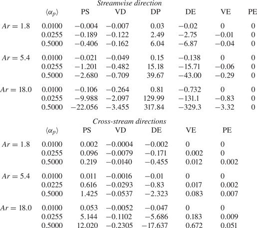


 Open access