


1 Introduction
Turbulent boundary-layer trailing-edge (TBL-TE) noise is produced by the scattering of hydrodynamic pressure fluctuations beneath a turbulent boundary layer at the trailing edge of an aerofoil (Amiet Reference Amiet1976; Howe Reference Howe1978). This is one of the major noise sources in wind turbines (Brooks, Pope & Marcolini Reference Brooks, Pope and Marcolini1989; Oerlemans, Sijtsma & López Reference Oerlemans, Sijtsma and López2007), which is often subject to curtailment for complying with noise regulations (Oerlemans et al. Reference Oerlemans, Fisher, Maeder and Kögler2009; Oerlemans Reference Oerlemans2016). In order to mitigate TBL-TE noise, various techniques have been proposed, such as acoustic optimization of aerofoil profiles (Marsden et al. Reference Marsden, Wang, Dennis and Moin2007) and trailing-edge add ons (e.g. serrations) (Oerlemans et al. Reference Oerlemans, Fisher, Maeder and Kögler2009; Gruber, Joseph & Chong Reference Gruber, Joseph and Chong2010; Arce León et al. Reference Arce León, Ragni, Pröbsting, Scarano and Madsen2016b; Avallone et al. Reference Avallone, van der Velden, Ragni and Casalino2018). Aside from these, open-cell porous materials have also been identified as promising concepts for both flow control (Sueki et al. Reference Sueki, Takaishi, Ikeda and Arai2010; Hasan, Foss & Sagatun Reference Hasan, Foss and Sagatun2012; Nair, Sameen & Lal Reference Nair, Sameen and Lal2018) and aerodynamic noise mitigation (Sarradj & Geyer Reference Sarradj and Geyer2007; Roger, Schram & De Santana Reference Roger, Schram and De Santana2013; Geyer & Sarradj Reference Geyer and Sarradj2014; Kim & Yoon Reference Kim and Yoon2015; Liu et al. Reference Liu, Azarpeyvand, Wei and Qu2015; Vathylakis, Chong & Joseph Reference Vathylakis, Chong and Joseph2015; Rubio Carpio et al. Reference Rubio Carpio, Avallone, Ragni, Snellen and van der Zwaag2019b).
Various studies were performed to assess the noise reduction capabilities of porous materials. Sarradj & Geyer (Reference Sarradj and Geyer2007) performed a comprehensive investigation about the relationship between the porous material properties (e.g. porosity and flow resistivity) and the acoustic response of fully porous SD7003 aerofoils. The porous aerofoils were observed to be quieter than their solid counterparts. However, no simple dependence between the material properties and the noise reduction level was found. Herr et al. (Reference Herr, Rossignol, Delfs, Lippitz and Mner2014) performed a parametric study on porous trailing edges to find the dependency of the noise reduction on the internal topology of porous materials. Different materials were considered, such as a micro-perforated plate, fibre felt, aluminium foam and sintered bronze powder. They observed that the noise reduction is higher for materials with smaller resistivity (i.e. larger permeability). Interestingly, the noise attenuation disappeared if one side of the porous trailing edge were covered with non-permeable tape. The authors hypothesized that the noise reduction mechanism was related to a pressure release process across the porous medium. More recently, Rubio Carpio et al. (Reference Rubio Carpio, Avallone, Ragni, Snellen and van der Zwaag2017) measured the acoustic response of a NACA 0018 equipped with porous trailing edge made of open-cell metal foam. The metal-foam trailing edge was applied at the last 20 % of the aerofoil chord, and the aerofoil was installed at zero angle of attack. The permeability of the porous trailing edge was varied by using metal foams of different pore sizes. They observed that the noise attenuation was higher for the porous trailing edge with larger pores (i.e. higher permeability), in line with the aforementioned studies (Geyer & Sarradj Reference Geyer and Sarradj2014; Herr et al. Reference Herr, Rossignol, Delfs, Lippitz and Mner2014). In a follow-up study, Rubio Carpio, Avallone & Ragni (Reference Rubio Carpio, Avallone and Ragni2018) and Rubio Carpio et al. (Reference Rubio Carpio, Avallone, Ragni, Snellen and van der Zwaag2019a) examined two different types of metal-foam trailing edge, referred to as the ‘permeable’ and ‘non-permeable’ porous trailing edges. The latter was manufactured by adding a layer of adhesive at the symmetry plane of the porous trailing edge, which completely blocked the metal-foam permeability in the wall-normal direction. In contrast to the aerofoil with a fully permeable trailing edge, there was no noise attenuation when the non-permeable variant was installed. The authors concluded that the flow field on both sides of the aerofoil had to be connected through the porous trailing edge to achieve noise reduction, which is in agreement with Herr et al. (Reference Herr, Rossignol, Delfs, Lippitz and Mner2014). However, the flow mechanism that was responsible for such behaviour has not been fully understood yet. This is partly due to the challenges associated with the instrumentation and measurement of the porous trailing edge. For instance, the installation of pressure transducers on the surface of the porous material poses the risk of perturbing the flow field (Showkat Ali, Azarpeyvand & Ilrio da Silva Reference Showkat Ali, Azarpeyvand and Ilrio da Silva2018). Moreover, flow-field measurements inside the porous material are relatively difficult to perform experimentally.
Numerical simulations might be able to overcome experimental limitations, particularly for obtaining flow quantities inside the porous medium. In the literature, there are various approaches for numerically resolving the flow field in porous material, such as by using an impedance boundary condition (Khorrami & Choudhari Reference Khorrami and Choudhari2003; Scalo, Bodart & Lele Reference Scalo, Bodart and Lele2015), or representing the porous medium as an equivalent fluid region (Whitaker Reference Whitaker1969; Koh, Meinke & Schröder Reference Koh, Meinke and Schröder2018; Zhou et al. Reference Zhou, Koh, Gauger, Meinke and Schöder2018). These approaches are often preferred over resolving the internal topology of porous media, as the latter might become prohibitively expensive if the pore dimensions are much smaller than the characteristic length of the body (Freed Reference Freed1998). For instance, Bruneau & Mortazavi (Reference Bruneau and Mortazavi2004) performed a direct numerical simulation to study the application of a porous coating to control the vortex shedding process of a square cylinder in cross-flow. The Navier–Stokes equations inside the porous medium was modified to include the Brinkman–Forchheimer–Darcy terms (also referred to as Hazen–Dupuit–Darcy terms) (Ingham & Pop Reference Ingham and Pop1998). A similar technique has been applied by Liu, Wei & Qu (Reference Liu, Wei and Qu2014) and Liu et al. (Reference Liu, Azarpeyvand, Wei and Qu2015) to investigate the effect of porous coating on isolated rod and tandem rod configurations. Koh et al. (Reference Koh, Meinke and Schröder2018) studied the application of porous material on a flat plate with blunt trailing edge using large eddy simulation (LES). Compared to the reference geometry, the porous treatment allowed for a noise reduction of up to 12 dB, particularly for the tonal noise component. The authors also showed that the impedance of the porous medium varies linearly with porosity and exponentially with porous structure size. More recently, the numerical application of a porous medium model on the sharp trailing edge of an airfoil was demonstrated by Bernicke et al. (Reference Bernicke, Akkermans, Bharadwaj, Ewert, Dierke and Rossian2018). The study involved a LES on a NACA 0012 aerofoil equipped with a porous trailing edge. Flow field in the porous medium region was modelled using a volume-averaging approach that took into account the effect of a friction term according to Darcy’s law. Subsequently, the aerofoil acoustic response as a single vortex convected over the trailing edge was measured; this was identical to the simulation set-up of Rossian, Ewert & Delfs (Reference Rossian, Ewert and Delfs2018). The permeability of the porous trailing edge was based on that of a perforated aluminium PA-80-110 as specified in Herr et al. (Reference Herr, Rossignol, Delfs, Lippitz and Mner2014). Compared to the solid trailing edge, the permeable variant showed substantial noise attenuation. Interestingly, the permeable trailing edge evidenced a secondary sound source at the solid–porous junction. Nevertheless, the physical mechanism behind the noise reduction was not explored further.
This manuscript aims at elucidating the noise reduction mechanism for a open-cell metal-foam trailing edge. In particular, this study examines the effect of material permeability on the noise scattering and flow-field behaviour of a porous trailing edge. Within this scope, the experimental study of Rubio Carpio et al. (Reference Rubio Carpio, Avallone and Ragni2018) is replicated numerically. The flow over a NACA 0018 aerofoil is computed by solving the explicit, transient and compressible Boltzmann equation, while the far-field sound is obtained using the Ffowcs Williams & Hawkings (Reference Ffowcs Williams and Hawkings1969) (FW-H) acoustic analogy. Moreover, the porous trailing edge is modelled using an equivalent fluid region approach based on Darcy’s law (Neuman Reference Neuman1977).
The rest of this manuscript is organized as follows. The numerical techniques, including the modelling of the porous material, are reported in § 2. The simulation cases are briefly presented in § 3. The simulation set-up is verified by the means of grid independence study, and validated against reference data in § 4. In-depth analyses of the far-field noise results are reported in § 5. Afterward, the effects of the porous trailing edge on the flow field are discussed in § 6. The findings are summarized in § 7, where an outlook is also provided.
2 Methodology
2.1 Flow solver
The flow field has been computed using the commercial solver PowerFLOW 5.4b based on the lattice-Boltzmann method (LBM). The methodology has also been used previously to predict TBL-TE noise (van der Velden, van Zuijlen & Ragni Reference van der Velden, van Zuijlen and Ragni2016; Avallone, Van der Velden & Ragni Reference Avallone, Van der Velden and Ragni2017; Avallone et al. Reference Avallone, van der Velden, Ragni and Casalino2018; Romani, van der Velden & Casalino Reference Romani, van der Velden and Casalino2018). The LB method describes the motion of fluid particles at mesoscopic scale and tracks the advection and collisions of fluid particles using distribution functions that are aligned with a finite number of predefined directions. These processes are described by the LB equation as follows:
 $$\begin{eqnarray}\frac{\unicode[STIX]{x2202}F}{\unicode[STIX]{x2202}t}+\boldsymbol{V}\boldsymbol{\cdot }\unicode[STIX]{x1D735}F=\boldsymbol{C},\end{eqnarray}$$
 where  $F(\boldsymbol{x},t)$ is the particle distribution function in spatial ( $\boldsymbol{x}$) and temporal space ( $t$),
$t$),  $\boldsymbol{V}$ is the particle velocity and $\boldsymbol{C}$ is the collision operator. The discretization of (2.1) involves 19 discrete velocity vectors in three dimensions (i.e. D3Q19) with a third-order truncation of the Chapman–Enskog expansion. This scheme has been shown to be accurate for approximating the Navier–Stokes equations for a perfect gas at low Mach number and isothermal conditions (Chen, Chen & Matthaeus Reference Chen, Chen and Matthaeus1992). The particle distribution function is solved on a Cartesian grid which is referred to as a lattice. The discretized form of the LB is written as
 $$\begin{eqnarray}F_{n}(\boldsymbol{x}+\boldsymbol{V}_{n}\unicode[STIX]{x0394}t,t+\unicode[STIX]{x0394}t)-F_{n}(\boldsymbol{x},t)=\boldsymbol{C}_{n}(\boldsymbol{x},t),\end{eqnarray}$$
 where  $F_{n}$ is the particle distribution function along the $n$th lattice direction, $\boldsymbol{V}_{n}$ is the discrete particle velocity in the $n$th direction. The collision term $\boldsymbol{C}_{n}$ follows the Bhatnagar–Gross–Krook model (Bhatnagar, Gross & Krook Reference Bhatnagar, Gross and Krook1954)
 $$\begin{eqnarray}\boldsymbol{C}_{n}=-\frac{\unicode[STIX]{x0394}t}{\unicode[STIX]{x1D70F}}[F_{n}(\boldsymbol{x},t)-F_{n}^{eq}(\boldsymbol{x},t)],\end{eqnarray}$$
 where  $\unicode[STIX]{x1D70F}$ is the relaxation time, which is a function of fluid viscosity and temperature, and $F_{n}^{eq}$ is the equilibrium distribution function of Maxwell–Boltzmann that is approximated with a second-order expansion (Chen et al. Reference Chen, Chen and Matthaeus1992) as
 $$\begin{eqnarray}F_{n}^{eq}=\unicode[STIX]{x1D70C}\unicode[STIX]{x1D714}_{n}\left[1+\frac{\boldsymbol{V}_{n}\boldsymbol{u}}{a_{s}^{2}}+\frac{(\boldsymbol{V}_{n}\boldsymbol{u})^{2}}{2a_{s}^{4}}-\frac{|\boldsymbol{u}|^{2}}{2a_{s}^{2}}\right],\end{eqnarray}$$
 where  $\unicode[STIX]{x1D714}_{n}$ are the fixed weight functions based on the D3Q19 model (Chen et al. Reference Chen, Chen and Matthaeus1992), and $a_{s}=1/\sqrt{3}$ is the non-dimensional speed of sound in lattice units. After solving (2.2) to obtain the distribution functions, macroscopic flow variables, such as density $\unicode[STIX]{x1D70C}$ and velocity $\boldsymbol{u}$, are computed as the discrete integration of the weighted distribution function over the state space as follows:
 $$\begin{eqnarray}\displaystyle & \displaystyle \unicode[STIX]{x1D70C}(\boldsymbol{x},t)=\mathop{\sum }_{n}F_{n}(\boldsymbol{x},t), & \displaystyle\end{eqnarray}$$
 $$\begin{eqnarray}\displaystyle & \displaystyle \unicode[STIX]{x1D70C}\boldsymbol{u}(\boldsymbol{x},t)=\mathop{\sum }_{n}\boldsymbol{V}_{n}F_{n}(\boldsymbol{x},t). & \displaystyle\end{eqnarray}$$
 The numerical solver adopts a very large eddy simulation (VLES) approach to consider the effects of the sub-grid unresolved scales of turbulence. The concept is based on the eddy viscosity model that is introduced into the collision term of the LB equation (Teixeira Reference Teixeira1998). This particular implementation employs a modified  $k-\unicode[STIX]{x1D716}$ (K-epsilon) two-equation turbulence model based on the renormalization group formulation. Turbulent fluctuations are taken into account by replacing the relaxation time $\unicode[STIX]{x1D70F}$ with an effective relaxation time $\unicode[STIX]{x1D70F}_{eff}$ as follows:
 $$\begin{eqnarray}\unicode[STIX]{x1D70F}_{eff}=\unicode[STIX]{x1D70F}+C_{\unicode[STIX]{x1D707}}\frac{k^{2}/\unicode[STIX]{x1D716}}{\sqrt{1+\unicode[STIX]{x1D702}^{2}}},\end{eqnarray}$$
 where  $C_{\unicode[STIX]{x1D707}}=0.09$ and $\unicode[STIX]{x1D702}$ are a combination of the local strain $k|\boldsymbol{S}/\unicode[STIX]{x1D716}|$, local vorticity $k|\unicode[STIX]{x1D74E}/\unicode[STIX]{x1D716}|$ and local helicity parameters. The modified relaxation time is used to calibrate the LB solver to the characteristic time scales of the turbulence in the flow field, which allows large scale vortical structures to develop. The unsteady nature of the LBM solution also implies that the resulting turbulence retains the history of the flow field. Moreover, it can be shown using the Chapman–Enskog expansion that the nonlinearity of the Reynolds stresses is captured (Teixeira Reference Teixeira1998; Chen et al. Reference Chen, Orszag, Staroselsky and Succi2004). Consequently, the LBM-VLES approach is substantially different than the Reynolds-averaged Navier–Stokes (RANS), despite similar turbulence transport equations being solved. The quantities derived from the turbulence model are not used to explicitly define Reynolds stresses, which are added to the system of governing equations in the case of RANS, but are only used to modify the relaxation properties of the system.
The cubic elements that constitute the lattice on which the LB scheme is carried out are referred to as voxels (i.e. volumetric pixels). The simulation domain can be subdivided into several regions where different voxel resolutions are applied, such that the resolution between two adjacent regions varies by a factor of 2. Solid boundaries are discretized using surfels (i.e. surface pixels) that are generated at locations where the voxels intersect solid surfaces. The wall boundary condition determines the appropriate fluid particle interaction description in the collision term of the LB scheme, such as a particle bounce-back process for a no-slip wall and specular reflection for a slip wall respectively (Chen, Teixeira & Molvig Reference Chen, Teixeira and Molvig1998). To further reduce computational cost for resolving the boundary layer at high Reynolds number, a wall model is applied on the first wall-adjacent grid (Teixeira Reference Teixeira1998; Wilcox et al. Reference Wilcox1998). The model is based on the generalized law-of-the-wall model (Launder & Spalding Reference Launder and Spalding1983), which has been extended to consider the effects of pressure gradient.
2.2 Far-field noise computations
The LB scheme is inherently unsteady and compressible with low dissipation and dispersion properties, which allows it to resolve the sound pressure field directly up to a cutoff frequency corresponding to approximately 15 voxels per acoustic wavelength. Due to this requirement, however, it is often more feasible to employ an acoustics analogy for obtaining far-field noise. In this study, far-field noise is computed using the FW-H analogy. In particular, the formulation 1A of Farassat & Succi (Reference Farassat and Succi1980) extended to a convective wave equation is used in this study (Brès, Pérot & Freed Reference Brès, Pérot and Freed2009). The formulation has been implemented in the time domain using a source-time dominant algorithm (Casalino Reference Casalino2003), which is extended to also allow integration on a permeable surface. Pressure fluctuations, including that on the surface of the porous medium, are recorded on the finest voxel resolution level (i.e. cutoff frequency ≈250 kHz). This approach considers a distribution of acoustic dipoles on the aerofoil surface (Curle Reference Curle1955), while other nonlinear contributions (e.g. turbulent aerofoil wake) are neglected. For comparison purposes, the FW-H analogy is also applied on a permeable surface enclosing the aerofoil, where the voxel resolution is two levels coarser than the finest one. The permeable surface is extended by  $2c$ downstream of the aerofoil trailing edge with the downstream face removed to avoid unwanted perturbations from the turbulent aerofoil wake (i.e. pseudo-noise associated with the suppression of the volume integral in the FW-H formulation) (Casper et al. Reference Casper, Lockard, Khorrami and Streett2004; Lockard & Casper Reference Lockard and Casper2005).
2.3 Numerical modelling of the porous medium
The porous medium has been modelled using an equivalent fluid region. This approach has the advantage of lowering computational costs when compared to fully resolving the internal topology of the porous medium. The equivalent fluid region mimics the presence of the porous medium by using an equivalent volume force, which depends on material properties as described by Darcy’s law (Neuman Reference Neuman1977). Consequently, the model resolves the spatially averaged effects of the flow-field interaction with the internal structures of the porous medium, similar to the methodology described in Bernicke et al. (Reference Bernicke, Akkermans, Bharadwaj, Ewert, Dierke and Rossian2018). The implementation of the porous medium model in PowerFLOW is briefly discussed in the following. For more details, readers are advised to refer to Freed (Reference Freed1998) and Sun et al. (Reference Sun, Pérot, Zhang, Lew, Mann, Gupta, Freed, Staroselsky and Chen2015).
Darcy’s law states that the pressure gradient  $\unicode[STIX]{x1D735}p$ for a flow permeating through a porous material is proportional to the transpiration velocity $\boldsymbol{u}$, as given in (2.8). This equation is also referred to as the Darcy force term (Rochette & Clain Reference Rochette and Clain2003).
 $$\begin{eqnarray}\unicode[STIX]{x1D735}p=-\unicode[STIX]{x1D70C}\boldsymbol{R}\boldsymbol{\cdot }\boldsymbol{u},\end{eqnarray}$$
 where  $\boldsymbol{R}$ is the flow resistivity, which consists of two components, namely the viscous resistivity $\boldsymbol{R}_{V}$ and the inertial resistivity $\boldsymbol{R}_{I}$; $\boldsymbol{R}$ can be further expanded as shown in (2.9). Substituting (2.9) into (2.8) results in an equation with both linear and nonlinear velocity terms that is equivalent to the Hazen–Dupuit–Darcy equation (also referred to as Brinkman–Forchheimer–Darcy equation) (Bear Reference Bear1972). Following this, $\boldsymbol{R}_{V}$ can be shown to be inversely proportional to the permeability $\boldsymbol{K}$, and $\boldsymbol{R}_{I}$ is equal to the form coefficient $\boldsymbol{C}$, as shown in (2.10).
 $$\begin{eqnarray}\boldsymbol{R}=\boldsymbol{R}_{V}+\boldsymbol{R}_{I}\boldsymbol{u},\end{eqnarray}$$
 $$\begin{eqnarray}\boldsymbol{R}_{V}=\frac{\unicode[STIX]{x1D707}}{\unicode[STIX]{x1D70C}\boldsymbol{K}},\quad \boldsymbol{R}_{I}=\boldsymbol{C}.\end{eqnarray}$$
It has been shown that the LB equations are equivalent to Navier–Stokes equations using the Chapman–Enskog expansion up to third-order truncation for perfect gas at low Mach number (Chen et al. Reference Chen, Chen and Matthaeus1992). Hence, equation (2.8) can be substituted to (2.2), and the resulting equation is equivalent to the following Navier–Stokes form:
 $$\begin{eqnarray}\displaystyle & \displaystyle \frac{\unicode[STIX]{x2202}\unicode[STIX]{x1D70C}}{\unicode[STIX]{x2202}t}+\unicode[STIX]{x1D735}\boldsymbol{\cdot }(\unicode[STIX]{x1D70C}\boldsymbol{u})=0, & \displaystyle\end{eqnarray}$$
 $$\begin{eqnarray}\displaystyle & \displaystyle \frac{\unicode[STIX]{x2202}\unicode[STIX]{x1D70C}\boldsymbol{u}}{\unicode[STIX]{x2202}t}+\unicode[STIX]{x1D735}\boldsymbol{\cdot }(\unicode[STIX]{x1D70C}\boldsymbol{u}\boldsymbol{u})=-\unicode[STIX]{x1D735}p-\unicode[STIX]{x1D70C}\boldsymbol{R}\boldsymbol{\cdot }\boldsymbol{u}, & \displaystyle\end{eqnarray}$$
where the regular viscous term in the Navier–Stokes equation has been replaced with the Darcy force term. Outside of the porous media region, however, the Darcy force term vanishes and it is replaced with the regular viscous term.
There are two slightly different porous medium models in PowerFLOW, namely the APM (acoustics porous medium) and the PM (porous medium). While both models describe porous media as equivalent fluid regions where the Darcy force term is applied, only the APM considers a physical interface between the regular fluid region and the porous medium region. On this interface, double-sided surfaces are applied similarly to a sliding mesh mechanism (Zhang et al. Reference Zhang, Sun, Li, Satti, Shock, Hoch and Chen2011). Additionally, the mass flow through the interface is governed by the mass-flux conservation as
 $$\begin{eqnarray}|\unicode[STIX]{x1D70C}\boldsymbol{u}\boldsymbol{\cdot }\boldsymbol{n}|_{\infty }=\unicode[STIX]{x1D719}|\unicode[STIX]{x1D70C}\boldsymbol{u}\boldsymbol{\cdot }\boldsymbol{n}|_{PM},\end{eqnarray}$$
 where  $\unicode[STIX]{x1D719}$ is the material porosity, $\boldsymbol{n}$ is a unitary normal vector at the interface, while the subscripts $\infty$ and $\text{PM}$ denote the regular fluid region and porous medium region, respectively. The porosity of the porous medium is defined as
 $$\begin{eqnarray}\unicode[STIX]{x1D719}=1-\frac{\unicode[STIX]{x1D70C}_{p}}{\unicode[STIX]{x1D70C}_{s}},\end{eqnarray}$$
 where  $\unicode[STIX]{x1D70C}_{p}$ and $\unicode[STIX]{x1D70C}_{s}$ are the overall density of the porous medium and that of the skeletal portion (matrix) of the sample, respectively.
It has been reported by Sun et al. (Reference Sun, Pérot, Zhang, Lew, Mann, Gupta, Freed, Staroselsky and Chen2015) that using empirical resistivity and porosity values is sufficient for resolving the aerodynamic and acoustic behaviours of rigid porous materials such as metal foam. However, PowerFLOW’s PM and APM models neglect other porous material properties, such as surface roughness and structural deformation. The latter can be neglected in the present case as the Ni-Cr-Al metal foam has been shown to be sufficiently rigid in experiments (Rubio Carpio et al. Reference Rubio Carpio, Avallone, Ragni, Snellen and van der Zwaag2017, Reference Rubio Carpio, Avallone, Ragni, Snellen and van der Zwaag2019b). Nevertheless, the surface roughness has been reported to cause noise increase at high frequency for aerofoils equipped with the porous trailing edge (Geyer & Sarradj Reference Geyer and Sarradj2014; Rubio Carpio et al. Reference Rubio Carpio, Avallone and Ragni2018). Hence, it is expected that the far-field noise of a porous aerofoil from the simulation will deviate from the trend of the experiment at high frequency where surface roughness effects become relevant.
3 Simulation set-up
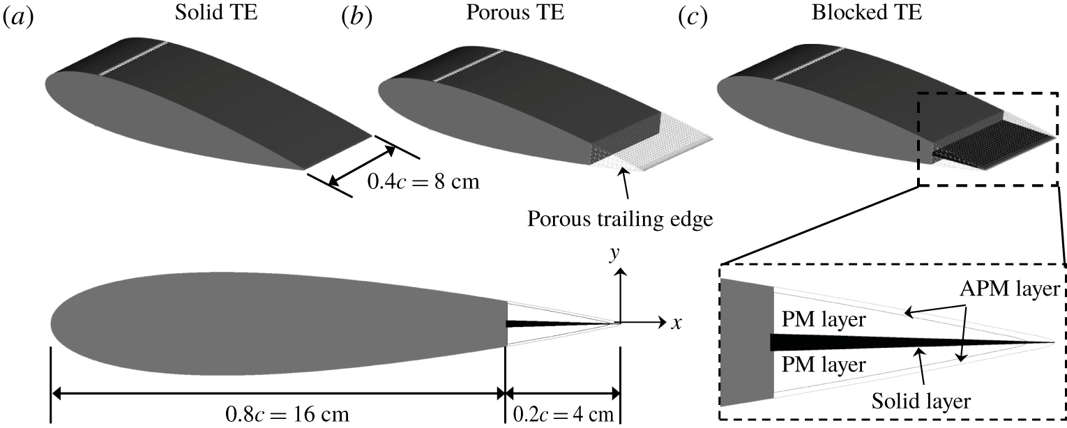
Figure 1. The NACA 0018 with three different trailing-edge (TE) configurations. The side view of the blocked TE is shown at the bottom left, where an inset shows the internal arrangement of the trailing-edge region of the blocked TE.
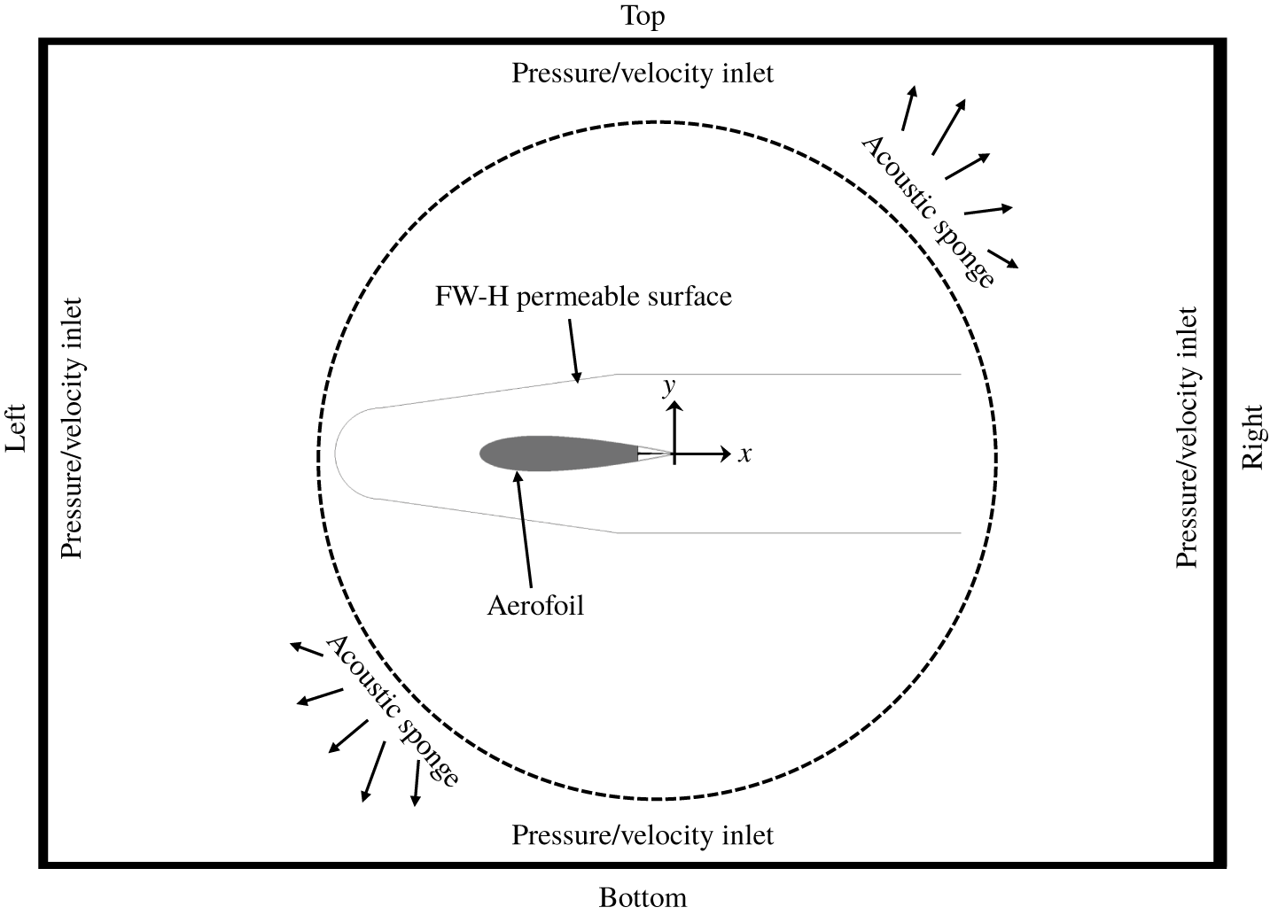
Figure 2. A sketch of the computational domain. The domain boundaries are not drawn to scale.
Present simulations replicate the experimental study of Rubio Carpio et al. (Reference Rubio Carpio, Avallone and Ragni2018). A NACA 0018, with chord equal to  $c=200~\text{mm}$ and span $b=80~\text{mm}$, is set at zero angle of attack. Three trailing-edge (TE) configurations are investigated: the baseline solid TE, the porous TE and the blocked TE. A sketch of the investigated configurations is provided in figure 1. For both porous and blocked TE cases, the porous medium model is applied at the last 20 % of the aerofoil chord length. The properties of the porous medium are based on the Ni-Cr-Al foam manufactured by Alantum. The characterization of the metal foam has been performed by Rubio Carpio et al. (Reference Rubio Carpio, Avallone, Ragni, Snellen and van der Zwaag2017), and its properties are reported in table 1. The mean cell diameter $d_{c}$ and porosity $\unicode[STIX]{x1D719}$ have been provided by the manufacturer while the permeability $K$ and form coefficient $\text{C}$ are obtained by curve fitting a series of pressure drop measurements with the Hazen–Dupuit–Darcy equation (Rubio Carpio et al. Reference Rubio Carpio, Avallone, Ragni, Snellen and van der Zwaag2017; Teruna et al. Reference Teruna, Manegar, Avallone, Casalino, Ragni, Rubio Carpio and Carolus2019). Furthermore, due to the random distribution of pores, the metal foam has isotropic and homogeneous properties. Note that the permeability and form coefficient listed in table 1 are asymptotic values, i.e. they are valid for a sample whose thickness is above a critical value (Dukhan & Minjeur Reference Dukhan and Minjeur2010).
Table 1. The metal-foam properties as measured by Rubio Carpio et al. (Reference Rubio Carpio, Avallone, Ragni, Snellen and van der Zwaag2017).
The porous trailing edge is represented as a combination of two equivalent fluid regions; the outer and inner volumes are modelled with the APM and PM models respectively. The APM layer follows the surface contour of the trailing edge with a constant thickness of 1 mm, except for the last  $0.005c$ of the aerofoil where the aerofoil thickness is less than 1 mm. The PM region lies underneath the APM layer. For the blocked TE, a solid core whose thickness equals to 12 % of the local trailing-edge thickness has been applied along the symmetry plane of the aerofoil (see the inset in figure 1). The solid core prevents any flow connection through the porous medium between both sides of the trailing edge (Rubio Carpio et al. Reference Rubio Carpio, Avallone, Ragni, Snellen and van der Zwaag2019b).
The combined APM-PM approach (see figure 1c) has been adopted in order to simplify the definition of  $R_{V}$ and $R_{I}$ at any given chordwise location, avoiding the need to specify both parameters locally depending on the thickness of the trailing edge. Dukhan & Patel (Reference Dukhan and Patel2010) and Baril et al. (Reference Baril, Mostafid, Lefebvre and Medraj2008) have reported that the resistivity of porous materials consists of two contributions: the bulk resistivity, which is independent of the sample thickness (i.e. asymptotic resistivity), and the thickness-dependent resistivity that is associated with the entrance/exit effect. In particular, the entrance/exit effect becomes more relevant as the sample thickness becomes comparable to the pore size. Nevertheless, this effect has been found to be limited to an entrance length, which is approximately equal to the pore diameter (Naaktgeboren, Krueger & Lage Reference Naaktgeboren, Krueger and Lage2004; Baril et al. Reference Baril, Mostafid, Lefebvre and Medraj2008). Beyond the entrance length, the flow is sufficiently steady such that the bulk resistivity dominates. Following this, the APM-PM combination takes into account the bulk resistivity with the PM core region and the entrance/exit effect with the APM layer (i.e. whose thickness is at least one pore diameter). The APM-PM combination has been previously verified by Teruna et al. (Reference Teruna, Manegar, Avallone, Casalino, Ragni, Rubio Carpio and Carolus2019) in which the pressure drop tests using the porous material characterization rig of Rubio Carpio et al. (Reference Rubio Carpio, Avallone, Ragni, Snellen and van der Zwaag2017) has been successfully replicated numerically.
The free-stream velocity is  $U_{\infty }=20~\text{ms}^{-1}$, which corresponds to a chord-based Reynolds number of $Re_{c}=280\,000$ and a free-stream Mach number of $M_{\infty }=0.06$. Zig-zag trips (Elsinga & Westerweel Reference Elsinga and Westerweel2012) have been installed at $x/c=-0.8$ on both sides of the aerofoil to force boundary-layer transition to turbulence. The zig-zag trip height is $t_{trip}=0.003c=0.6~\text{mm}$, while the amplitude is $c_{trip}=0.015c=3~\text{mm}$ and the wavelength is $\unicode[STIX]{x1D706}_{trip}=0.015c=3~\text{mm}$. The tripping elements are the same as those used in a similar study (Avallone et al. Reference Avallone, van der Velden, Ragni and Casalino2018).
The sketch of the computational domain is shown in figure 2. The origin of the coordinate system is located at the mid-span of the trailing edge with the  $x$ axis aligned with the aerofoil chord, the $z$ axis with the aerofoil span and the $y$ axis is perpendicular to both the $x$ and $z$ axes. For the rest of this manuscript, the positive $x$ direction will also be referred to as the streamwise direction, whereas the $y$ and $z$ axes are in the vertical and spanwise directions respectively. The computational domain is a rectangular box whose dimensions equal to $100c$ in both the $x$ and $y$ directions and $b$ in the spanwise direction. An acoustic sponge region is specified, starting from a radius of $36c$ from the origin, to damp outward-travelling and inward-reflected acoustic waves. Periodic boundary conditions are applied on the lateral faces of the simulation domain. A total of 10 grid refinement regions with a resolution factor of 2 are employed with the finest grid region being applied adjacent to the aerofoil surface. As a result, the smallest voxel has a dimension of $3.9\times 10^{-4}c$, which guarantees that there are at least 10 grid points across the APM layer (Sun et al. Reference Sun, Pérot, Zhang, Lew, Mann, Gupta, Freed, Staroselsky and Chen2015) along the trailing edge. For the aerofoil with the solid trailing edge, the finest voxel resolution corresponds to the first wall-adjacent cell height of $y^{+}=3$ surrounding the trailing edge. The discretization results in a total of 218 × 106 and 293 × 106 voxels inside the simulation domain for the solid and porous trailing-edge cases, respectively. The simulation has been carried out for 20 flow passes, excluding the initial transient, during which pressure fluctuations on the surface and on the permeable FW-H surface are sampled at 150 kHz for far-field noise computations. The simulations have been run on the servers of University of Siegen with the porous TE case requiring a total of 27 000 CPU hours on a 320-core Xeon E5-2630 v3 platform.
4 Grid independence study and validation against experiments
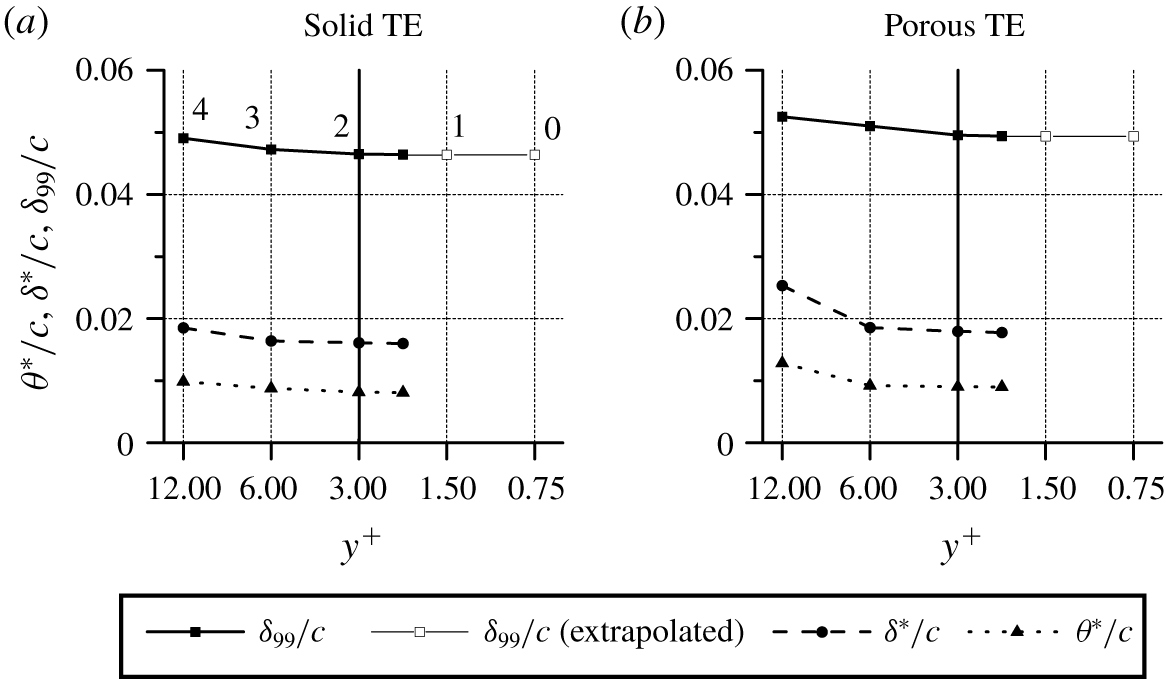
Figure 3. The comparison of boundary-layer thickness at  $x/c=-0.002$ for different grid resolutions. The Richardson extrapolation of the boundary-layer thickness is plotted as an empty square. The thick line at $y^{+}=3$ denotes the adopted grid resolution for the rest of the manuscript. The corresponding resolution levels that are considered for the grid convergence index ( $GCI$) studies are numbered next to the data point.
Table 2. Comparison of boundary-layer properties on the solid trailing edge ( $x/c=-0.02$) against previous experimental and numerical studies.
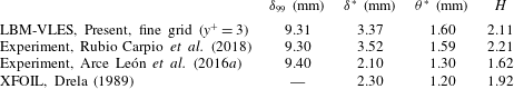
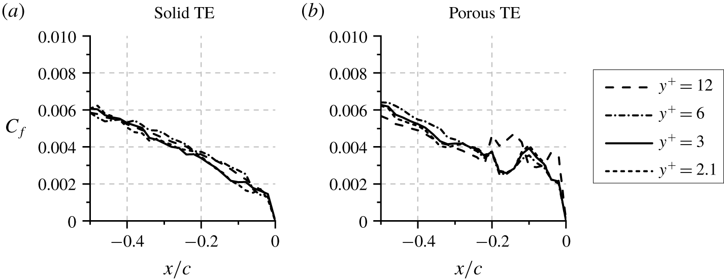
Figure 4. The comparison of wall-friction coefficients at  $x/c>-0.5$ for different grid resolutions.
A grid independence study has been performed. Four grid resolutions are considered: coarse ( $y^{+}=12$), medium ( $y^{+}=6$), fine ( $y^{+}=3$) and very fine ( $y^{+}=2.12$). This is achieved by uniformly increasing the resolution of each refinement region. The integral boundary-layer parameters, such as boundary-layer thickness ( $\unicode[STIX]{x1D6FF}_{99}$), displacement thickness ( $\unicode[STIX]{x1D6FF}^{\ast }$) and momentum thickness ( $\unicode[STIX]{x1D703}^{\ast }$), are used for the convergence analysis, as shown in figure 3. The boundary-layer thickness is defined as $U(\unicode[STIX]{x1D6FF}_{99})=0.99U_{e}$, where $U_{e}$ is the velocity at the boundary-layer edge ( $\unicode[STIX]{x1D6FF}_{e}$) defined as the position where the integral of the spanwise vorticity along the wall-normal direction (i.e. $\int \unicode[STIX]{x1D714}_{z}\,\text{d}y$) is asymptotic (Spalart & Watmuff Reference Spalart and Watmuff1993). This procedure is also applied for the porous and blocked TE cases although the conventional no-slip condition is not applicable on the porous surface (Delfs et al. Reference Delfs, Faßmann, Lippitz, Lummer, Mößner, Müller, Rurkowska and Uphoff2014; Rubio Carpio et al. Reference Rubio Carpio, Avallone, Ragni, Snellen and van der Zwaag2019b). The Richardson extrapolations of the boundary-layer thicknesses, excluding $y^{+}=2.12$, are also plotted in figure 3 as empty square markers for $y^{+}=1.5$ and 0.75, in which the refinement ratio is $r=2$ and the order of convergence is $p=3$. The figure verifies that the results for $y^{+}=2.12$ lie along the extrapolation line.
The grid convergence index ( $GCI$) of the boundary-layer thickness is computed to further ascertain the convergence of the simulation results. The grid resolution level is indicated next to the data points of $\unicode[STIX]{x1D6FF}_{99}/c$ in figure 3(a). For the solid trailing edge, $GCI_{2,3}=0.288\,\%$ and $GCI_{1,2}=0.0385\,\%$, whereas for the porous trailing edge, $GCI_{2,3}=0.519\,\%$ and $GCI_{1,2}=0.0687\,\%$. Thus, the $GCI$ ratios, which are computed as in (4.1), are 0.935 and 0.944 for the solid and porous trailing edges, respectively. The small $GCI$ values and the $GCI$ ratios being close to unity, indicate that the selected grid resolutions are within the asymptotic range of convergence.
 $$\begin{eqnarray}GCI_{ratio}=\frac{GCI_{2,3}}{r^{p}GCI_{1,2}}.\end{eqnarray}$$
 Grid convergence is also evaluated based on the trend of wall-friction coefficient ( $C_{f}$) in figure 4. Qualitatively, the $C_{f}$ distribution for solid TE does not appear to vary significantly with the grid resolution. Conversely, the plot for porous TE case shows a large discrepancy between $y^{+}=12$ and $y^{+}=6$ results. This can be attributed to the under-resolved APM layer, which is represented only by 3 voxels for the coarser grid setting. For finer grid resolutions, the $C_{f}$ distribution for porous TE converges. Thus, the grid independence study indicates that a voxel resolution corresponding to $y^{+}=3$ is sufficient and thus, this setting has been chosen for the rest of this manuscript.
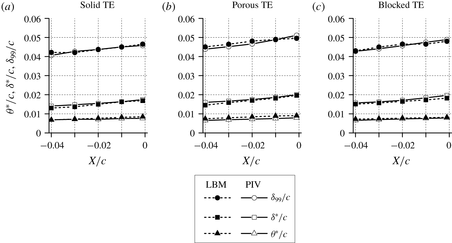
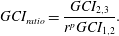
Figure 5. The integral boundary-layer parameters along the last 4 % of the aerofoil chord. Experimental particle image velocimetry (PIV) data are taken from Rubio Carpio et al. (Reference Rubio Carpio, Avallone and Ragni2018).
Figure 6. Profiles of the time-average ( $U$) and the root-mean-square of the wall-parallel ( $\sqrt{\overline{u^{2}}}$) and of the wall-normal ( $\sqrt{\overline{v^{2}}}$) velocity components at $x/c=0$. Experimental data are extracted from Rubio Carpio et al. (Reference Rubio Carpio, Avallone and Ragni2018, Reference Rubio Carpio, Avallone, Ragni, Snellen and van der Zwaag2019b) and Arce León et al. (Reference Arce León, Merino-Martínez, Ragni, Avallone and Snellen2016a).
Computational results are also compared against the experimental measurements of Arce León et al. (Reference Arce León, Merino-Martínez, Ragni, Avallone and Snellen2016a) and Rubio Carpio et al. (Reference Rubio Carpio, Avallone and Ragni2018). Table 2 shows the comparison of  $\unicode[STIX]{x1D6FF}_{99}$, $\unicode[STIX]{x1D6FF}^{\ast }$, $\unicode[STIX]{x1D703}^{\ast }$ and the shape factor $H$ for the solid trailing edge at $x/c=-0.02$. While the results of the current simulation are comparable to the experiments, there are small discrepancies which are likely attributed to the different tripping elements (i.e. zig-zag trip in the simulation and carborundum particles in the experiments). The spatial development of the boundary-layer parameters is also examined along the last 4 % of the aerofoil chord, as shown in figure 5. For all three different trailing-edge treatments studied, good agreement is obtained between present results and experimental ones. For instance, the thickening of the boundary layer associated with the porous medium permeability is also captured by the simulation (Geyer & Sarradj Reference Geyer and Sarradj2014; Rubio Carpio et al. Reference Rubio Carpio, Avallone and Ragni2018, Reference Rubio Carpio, Avallone, Ragni, Snellen and van der Zwaag2019b; Teruna et al. Reference Teruna, Manegar, Avallone, Casalino, Ragni, Rubio Carpio and Carolus2019). Similar agreement has also been found for the mean and turbulent velocity profiles as shown in figure 6. The mean velocity deficit caused by the permeability of the porous trailing edge is slightly underpredicted, which is also reflected by the lower $\unicode[STIX]{x1D6FF}^{\ast }$ in table 2. This is conjectured to be due to the neglected surface roughness since the discrepancy is more prominent near the wall. Nevertheless, the turbulent velocity fluctuation trends are still captured by the numerical results, suggesting that the zig-zag tripping elements, combined with the two-layer PM-APM approach, are capable of reproducing similar boundary-layer characteristics as in the experiments.
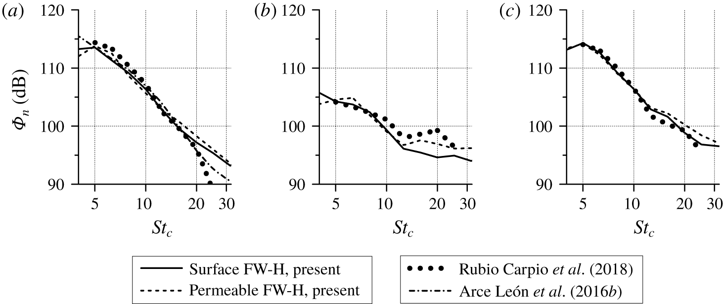
Figure 7. Normalized one-third octave far-field sound spectra  $\unicode[STIX]{x1D719}_{n}$ of the (a) solid, (b) porous and (c) blocked trailing edges. Experimental data are extracted from Arce León et al. (Reference Arce León, Ragni, Pröbsting, Scarano and Madsen2016b) and Rubio Carpio et al. (Reference Rubio Carpio, Avallone and Ragni2018).
The far-field noise trends are also validated against the experiments, to assess whether the porous medium model allows an accurate prediction of the sound generated by the porous trailing edge. Far-field noise computations are performed with the FW-H analogy using the pressure fluctuations sampled on the aerofoil surface and on a permeable surface enclosing the aerofoil. Subsequently, the Fourier analysis is performed using a periodogram method (Welch Reference Welch1967) with Hanning windowing and the resulting spectra are reported in third octave bands. Far-field sound is computed at  $x=0,y=7.4c,z=0$, where the $y$ coordinate corresponds to the distance of the microphone array from the trailing edge in the experiment (Rubio Carpio et al. Reference Rubio Carpio, Avallone and Ragni2018). The raw sound spectra $\unicode[STIX]{x1D6F7}_{o}$ are scaled to a reference observer distance $D=1~\text{m}$, span $b=1~\text{m}$ and Mach number $M=1$, which has been enforced with the fifth-power law (Ffowcs Williams & Hawkings Reference Ffowcs Williams and Hawkings1969; Blake Reference Blake1986). The scaling procedure is expressed as in (4.2) (van der Velden et al. Reference van der Velden, van Zuijlen and Ragni2016; Avallone et al. Reference Avallone, van der Velden, Ragni and Casalino2018).
 $$\begin{eqnarray}\unicode[STIX]{x1D6F7}_{n}=\unicode[STIX]{x1D6F7}_{o}+20\text{log}_{10}(D)-10\text{log}_{10}(b)-50\log _{10}(M_{\infty }).\end{eqnarray}$$
 The scaled sound spectra ( $\unicode[STIX]{x1D6F7}_{n}$) for each trailing-edge treatment are shown in figure 7. The results from the surface FW-H and permeable FW-H formulations are also compared in the plots. For the solid TE case (figure 7a), both methods produce similar spectra with a maximum difference of 1 dB at $St_{c}=17.5$. The spectra are also in good agreement with experimental measurements, with discrepancies appearing only above $St_{c}=22$. Spectra from different experimental datasets also show deviations in this frequency range, which might be due to the influence of the different tripping elements (Ye et al. Reference Ye, Avallone, Ragni, Choudhari and Casalino2019). For the porous TE case, the surface and permeable FW-H results show a small difference (i.e. ≈2 dB) at frequencies above $St_{c}=12$. This discrepancy can be attributed to the neglected contribution of monopole sources in the surface FW-H formulation (i.e. the unsteady flow injection and ejection at the porous medium surface (Nelson Reference Nelson1982)). This source term appears to be noticeable only in the high frequency range but not at low frequencies where most of the noise attenuation is obtained. Hence, the results of the surface FW-H formulation can also be used for investigating the noise reduction mechanisms of the porous TE. Nonetheless, the sound spectra obtained from the simulation still underpredict the experimental data. This is attributed to the surface roughness noise contribution that is not considered by the simulation. Good agreement with the reference data is obtained for the blocked TE case, in which the numerical result shows that the noise reduction at low frequencies is not present. This confirms that the flow fields on both sides of the porous trailing edge have to remain connected through the porous medium to attenuate noise, which is also in line with the findings of Herr et al. (Reference Herr, Rossignol, Delfs, Lippitz and Mner2014), Rubio Carpio et al. (Reference Rubio Carpio, Avallone and Ragni2018) and Rubio Carpio et al. (Reference Rubio Carpio, Avallone, Ragni, Snellen and van der Zwaag2019a).
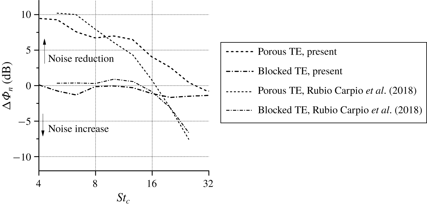
Figure 8. The difference in sound spectra  $\unicode[STIX]{x0394}\unicode[STIX]{x1D6F7}_{n}$ for different trailing-edge variants with respect to the solid case. Experimental data are extracted from Rubio Carpio et al. (Reference Rubio Carpio, Avallone and Ragni2018).
The difference in the far-field noise produced by the porous trailing edges (i.e. porous and blocked TE) and the solid one is expressed as  $\unicode[STIX]{x0394}\unicode[STIX]{x1D6F7}_{n}=\unicode[STIX]{x1D6F7}_{n,solid}-\unicode[STIX]{x1D6F7}_{n,porous}$ and plotted in figure 8. The experimental results reported in Rubio Carpio et al. (Reference Rubio Carpio, Avallone and Ragni2018) are also provided for comparison. The figure evidences that the trends of the experiment have been captured by the simulation, although discrepancies are present at high frequency. The porous TE still shows noise reduction up to $St_{c}=30$, while the noise increase caused by the blocked TE remains smaller than 2 dB. This further corroborates that the excess noise at high frequency produced by the porous TE can be associated with the increase in surface roughness, which cannot be replicated in the simulation using the present equivalent fluid region approach.
This section has shown that the simulations using the porous medium model are able to reproduce the general aeroacoustic trends of the porous trailing-edge applications observed in experiments. Further analyses on noise reduction mechanisms of the porous trailing edge are reported in the subsequent sections. The results from the surface FW-H method are presented hereafter unless otherwise indicated.
5 Effects of the porous trailing-edge treatment on trailing-edge noise
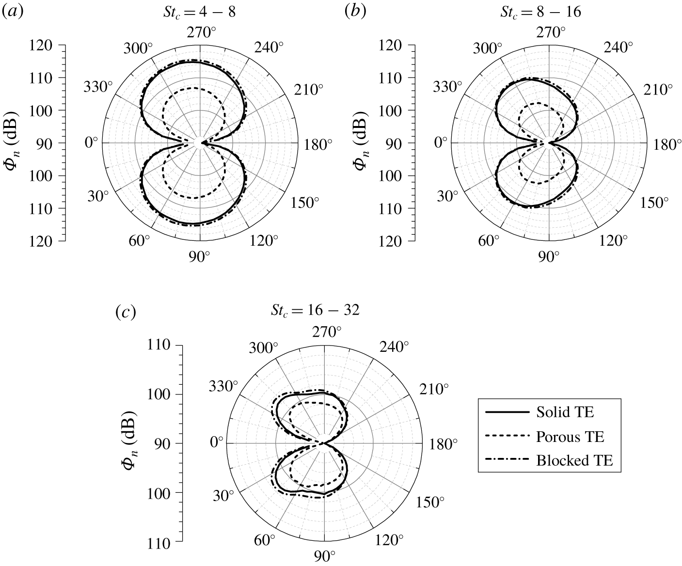
Figure 9. Directivity of the far-field sound spectra  $\unicode[STIX]{x1D719}_{n}$ for the solid, porous and blocked trailing-edge cases, plotted in three different frequency ranges (a) $4<St_{c}<8$, (b) $8<St_{c}<16$ and (c) $16<St_{c}<32$. The aerofoil leading edge is facing towards $0^{\circ }$.
5.1 Far-field noise directivity and noise source localization
The application of the porous material at the trailing edge might alter far-field sound radiation pattern. Thus, the sound directivity for the three cases is shown in figure 9. The plots are obtained using 72 virtual microphones that are equally spaced on a circle in the  $x{-}y$ plane with a radius of $7.4c$ from the trailing-edge mid-span. The sound spectra are further integrated into three frequency bands corresponding to the noise reduction characteristics of the porous TE observed in the experiments (Rubio Carpio et al. Reference Rubio Carpio, Avallone and Ragni2018, Reference Rubio Carpio, Avallone, Ragni, Snellen and van der Zwaag2019a), i.e. at $4<St_{c}<8$ where the noise reduction is the highest, at $8<St_{c}<16$ which is a transitional region where the noise reduction becomes smaller and at $16<St_{c}<32$ where the noise reduction is no longer observed.
The sound directivity at low frequency (figure 9a) for all three cases resembles that of a compact dipole. This dipole is tilted towards the leading edge in the mid-frequency range (figure 9b) (Oerlemans et al. Reference Oerlemans, Fisher, Maeder and Kögler2009; Roger & Moreau Reference Roger and Moreau2010). Non-compact behaviours start to appear at higher frequencies (figure 9c), in which two lobes can be identified for the solid and blocked TE cases. The noise reduction due to the porous TE is evident in all three frequency ranges, with the largest reduction being achieved between  $30^{\circ }$ and $60^{\circ }$. On the other hand, the blocked TE exhibits a slight noise increase in the highest frequency band when compared to the solid TE. Nonetheless, the plots show that the far-field directivity shape is not significantly affected by the presence of the porous TE nor the blocked TE. Moreover, the directivity plots suggest that the noise generation mechanism for all three cases is similar.
A conventional beamforming algorithm (a tool developed by Dassault Systemes that has been benchmarked against other beamforming methods (Lockard et al. Reference Lockard, Humphreys, Khorrami, Fares, Casalino and Ravetta2017)) is employed to ascertain the location of dominant noise sources. The virtual microphone array that is used in this study is based on the Underbrink’s spiral array configuration (Underbrink Reference Underbrink2001), as shown in figure 10. It is a modification of the 64-microphone array that has been used previously by Rubio Carpio et al. (Reference Rubio Carpio, Avallone and Ragni2018), whose Rayleigh limit is approximately equal to  $c$ at $St_{c}=12.5$ in the chordwise direction. In order to increase the spatial resolution (i.e. to decrease the Rayleigh limit) with respect to the existing antenna, this study considers a larger one consisting of 320 microphones. The antenna is built using 5 concentric arrays with 64 microphones each, in which the innermost array is the same as that used by Rubio Carpio et al. (Reference Rubio Carpio, Avallone and Ragni2018) (see figure 10b). The resulting antenna has an overall dimension of $200c\times 4c$ and the Rayleigh limit is approximately equal to $0.1c$ in the chordwise direction at $St_{c}=12.5$. This allows distinguishing of the noise sources at the solid–porous junction and the trailing edge for both porous and blocked TE cases provided that the sources at both locations have comparable intensity.
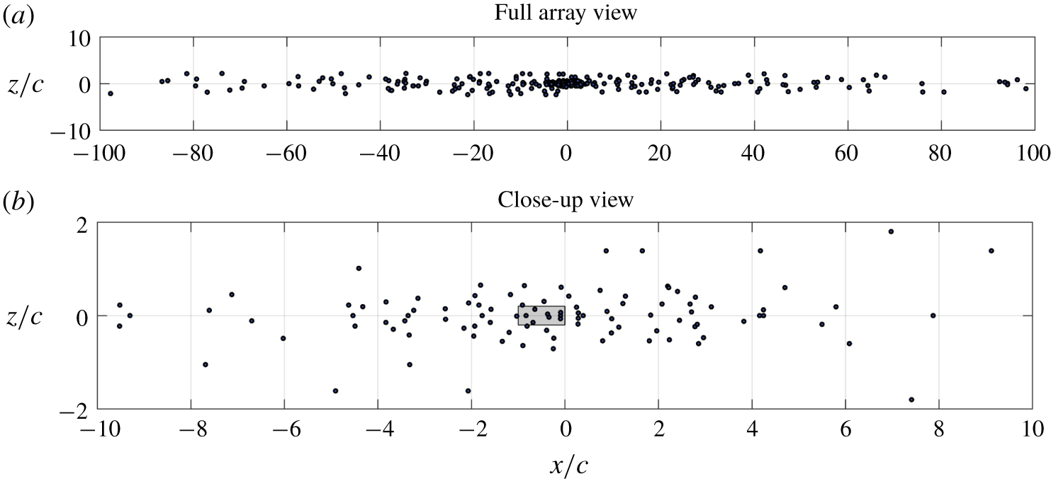
Figure 10. The distribution of 320 microphones in a modified Underbrink (Reference Underbrink2001) configuration. The grey area represents the planform of the aerofoil with the flow towards the positive  $x$ direction.
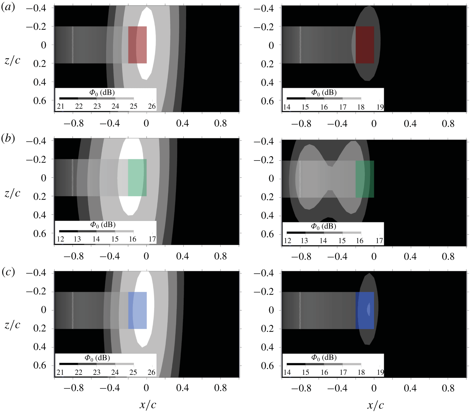
Figure 11. Source maps for one-third octave band, centred at 1250 Hz ( $St_{c}=12.5$) (left column) and 2500 Hz ( $St_{c}=25$) (right column) for the (a) solid, (b) porous and (c) blocked TE cases. The trailing-edge region ( $-0.2<x/c<0$) for each respective case is highlighted in different colours.
The source maps for the one-third octave band centred at  $St_{c}=12.5$ (left column) and $St_{c}=25$ (right column) are shown in figure 11. At $St_{c}=12.5$, the source of maximum noise generation for the solid TE is aligned with the trailing edge, similar to the case of the blocked TE. For the porous TE, on the other hand, the location of the maximum noise intensity shifts towards the solid–porous junction (i.e. $x/c=-0.2$). Although it has been reported (Herr et al. Reference Herr, Rossignol, Delfs, Lippitz and Mner2014; Bernicke et al. Reference Bernicke, Akkermans, Bharadwaj, Ewert, Dierke and Rossian2018; Kisil & Ayton Reference Kisil and Ayton2018) that the porous TE might still scatter noise from the trailing edge in addition to the solid–porous junction, the source map of the porous TE implies that the acoustic scattering at the actual trailing edge is weaker than that at the solid–porous junction. At $St_{c}=25$, the source map of the porous TE shows an additional source nearby the zig-zag trip in addition to the solid–porous junction. The sources nearby the tripping device do not appear in other source maps due to the lower relative intensity. These results are in line with the observations of Rubio Carpio et al. (Reference Rubio Carpio, Avallone, Ragni, Snellen and van der Zwaag2019b), who suggested that the locations where noise is primarily scattered are influenced by the trailing-edge permeability. A further look into the acoustic scattering on the different trailing-edge treatments will provide better insights into this matter.
5.2 Acoustic scattering analyses
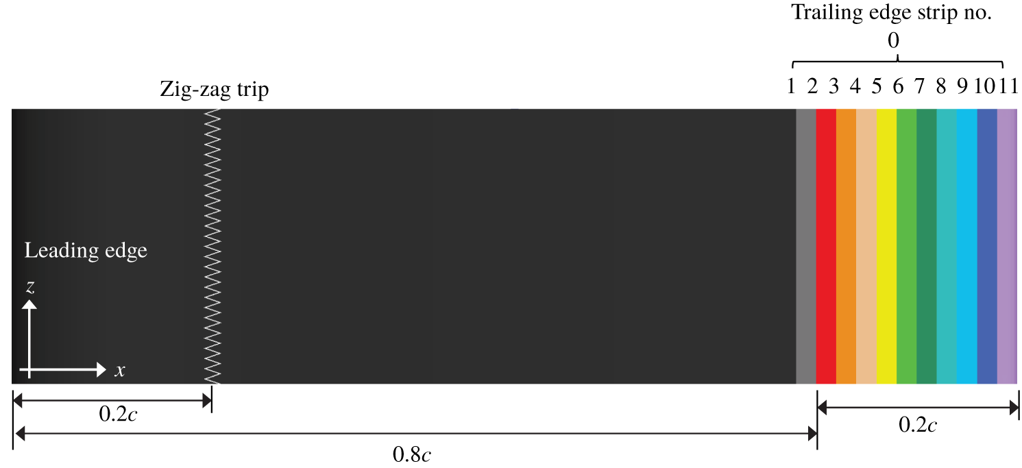
Figure 12. The arrangement of the trailing-edge strips for acoustic scattering analysis.
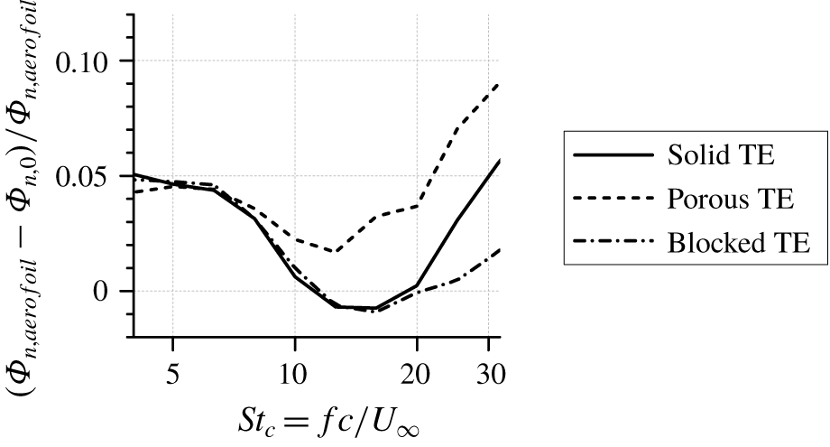
Figure 13. The difference between the noise generated by the entire aerofoil ( $\unicode[STIX]{x1D6F7}_{n,aerofoil}$) and that of strip 0 ( $\unicode[STIX]{x1D6F7}_{n,0}$), i.e. the noise contribution of the aerofoil segment upstream of strip 0.
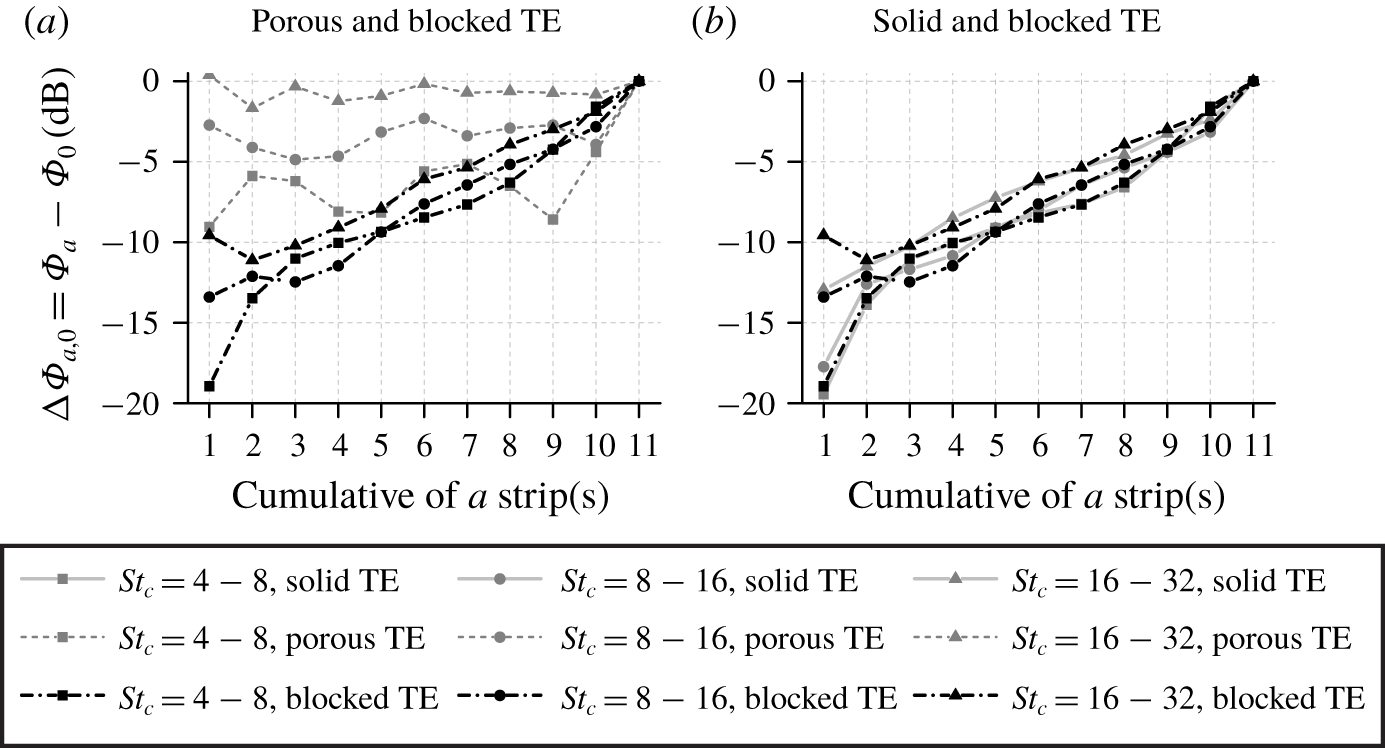
Figure 14. The relative difference between the cumulative sum of the noise contribution from a selected number of strips (i.e.  $1,1{-}2,\ldots ,1{-}11$) and that of the entire 11 strips.
In the previous subsection, the porous TE was shown to scatter less noise compared to the solid TE, while the blocked TE shows no noise reduction. Moreover, the beamforming maps have indicated that the location of dominant noise source for the porous TE is different to those of the solid and blocked TE. To help understanding this behaviour, this subsection examines the effects of the trailing-edge treatments on the distribution of sound sources on the aerofoil surface.
In order to quantify the far-field noise contribution of each segment of the trailing-edge region, the last 22 % of the chord has been divided into 11 strips, as shown in figure 12. The procedure is carried out using a virtual microphone located directly above the TE (i.e.  $x/c=0,y/c=7.4$). The analysis of the cumulative sum of the far-field noise contribution from the strips allows detecting of regions with a major contribution to the overall far-field noise, while cross-correlation analyses between the strips provide the phase relations (i.e. constructive and destructive interference) between the scattered sound waves. Each strip is $0.02c$ long, which has been verified to be larger than the streamwise correlation length of surface pressure fluctuations at any given location for all of the trailing-edge variants. This is to ensure that each strip can be assumed to be an independent sound source. A similar analysis has been carried out by Avallone et al. (Reference Avallone, van der Velden, Ragni and Casalino2018) for studying the scattering mechanism of trailing-edge serrations. On the porous and blocked TE, strips 2–11 are located on the porous medium region, whereas strip 1 remains on the solid segment of the aerofoil. Additionally, strip 0 is used to designate the combined contribution of all the strips.
Figure 13 shows the far-field noise contribution of the aerofoil segment upstream of strip 0 (i.e. upstream of the last 22 % of the chord length) relative to the total noise. For all three TE configurations, the region upstream of strip 0 contributes to less than 10 % to the overall noise in the entire frequency range of interest. This verifies that trailing-edge noise remains the dominant source of noise. For all cases, the larger contribution from the upstream part of the aerofoil at high frequencies could be attributed to the self-noise of the zig-zag trip (van der Velden et al. Reference van der Velden, van Zuijlen, de Jong and Ragni2017). The trends of the solid and blocked TE are similar up to  $St_{c}=13$, which corresponds to the frequency where the blocked TE starts to exhibit noise increase (see figure 8). This implies that the far-field noise contribution of the aerofoil main body is similar in both cases.
The cumulative sum of the far-field noise contribution from each strip is shown in figure 14. The cumulative sum is plotted relative to the overall noise produced by all the strips  $\unicode[STIX]{x1D6F7}_{0}$ (i.e. $\unicode[STIX]{x0394}\unicode[STIX]{x1D6F7}_{a,0}=\unicode[STIX]{x1D6F7}_{a}-\unicode[STIX]{x1D6F7}_{0}$). A positive slope indicates that the noise contribution of a particular strip is in phase with the sum of the previous strips, whereas an out-of-phase contribution is reflected as a negative slope. Interestingly, the trend for the solid TE is similar to that of the blocked TE as shown in plot (b), except for strips 1–3 at higher frequencies ( $8<St_{c}<32$). This is consistent with the findings in figures 8 and 13. Meanwhile, (a) shows that, for all three frequency bands, the far-field noise contribution from the solid–porous junction is more dominant for the porous TE than for the blocked TE (i.e. ≈10 dB), similar to what is shown in the acoustic source maps (figure 11); for the blocked TE, the sound generated by the solid–porous junction is relevant only at higher frequencies. The cumulative sum of the blocked TE shows an uphill trend as a higher number of strips are considered, which implies that most of the strips are in phase with one another. In contrast, the porous TE shows more slope variation, which indicates the presence of out-of-phase relationships (i.e. destructive interference) between the strips. It is also notable that $\unicode[STIX]{x0394}\unicode[STIX]{x1D6F7}_{a,0}$ for the porous TE exhibits larger slope variations at lower frequency. Since a steeper slope indicates more intense interference between one strip and the others, this might justify the larger low frequency noise reduction of the porous TE.
Correlation analyses are carried out to elucidate the interference phenomena of the scattered acoustic waves. The time-domain cross-correlation between the far-field noise contribution from different strips and that of strip 0  $R_{a,0}(\unicode[STIX]{x0394}t)$ is computed as
 $$\begin{eqnarray}R_{a,0}(\unicode[STIX]{x0394}t)=\frac{\langle p_{a}(t+\unicode[STIX]{x0394}t)p_{0}(t)\rangle }{\sqrt{\langle p_{a}^{2}(t)\rangle }\sqrt{\langle p_{0}^{2}(t)\rangle }},\end{eqnarray}$$
 where  $p_{a}$ and $p_{0}$ are the time histories of the acoustic pressure produced by strip $a$ and strip $0$ respectively, $\unicode[STIX]{x0394}t$ is the temporal lag and $\langle \cdot \rangle$ is an ensemble-average operator. The maximum value of $R_{a,0}(\unicode[STIX]{x0394}t)$ and the corresponding lag $\unicode[STIX]{x0394}t$ are plotted in figure 15. The quantity $\max (R_{a,0}(\unicode[STIX]{x0394}t))$ indicates the relative noise contribution by a strip compared to that of strip 0, while the presence of temporal lag implies a partial interference between the acoustic pressure produced by a particular strip and the total contribution of the 11 strips.
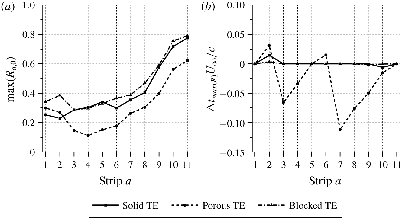
Figure 15. (a) The maximum value of cross-correlation between the far-field noise contribution of an individual strip and that of strip 0, and (b) the corresponding non-dimensional temporal lag.
Figure 15(a) shows a higher correlation at the solid–porous junction (i.e. strips 1 and 2) of the porous and blocked TE than that for the solid TE. It is also evident that the correlation level at strips 10 and 11 (i.e. last 2 % of the chord) of the porous TE is lower than that of the solid and blocked TE. This implies that the scattering at the trailing edge of the porous TE is less intense compared to that of the solid or blocked TE ones. Starting from strip 3, the blocked TE shows a very similar trend to the solid TE with the correlation level increasing towards the trailing-edge location. Conversely, the correlation level for the porous TE case exhibits an immediate reduction, in particular between strips 3 and 7, before showing a positive slope. These behaviours can be linked to the temporal lag plots in figure 15(b). The temporal lag trends show that individual strips of the solid and blocked TE are strongly in phase with strip 0. On the other hand, the trend of the porous TE clearly shows significant lag for the majority of the strips. This suggests that the sound waves emitted by different strips have different phase, which promotes destructive interference that contributes to noise attenuation.
The cross-correlation analysis is also extended to the frequency domain. The cross-spectral density (CSD) between the strips is computed and it is presented as matrices in figure 16. The CSD is defined as in (5.2)
 $$\begin{eqnarray}C_{a,b}(\unicode[STIX]{x1D714})=\int _{-\infty }^{\infty }\left[\int _{-\infty }^{\infty }p_{a}(t)p_{b}(t+\unicode[STIX]{x0394}t)\,\text{d}\unicode[STIX]{x0394}t\right]\text{e}^{\text{i}\unicode[STIX]{x1D714}t}\,\text{d}t,\end{eqnarray}$$
 where  $p_{a}(t)$ and $p_{b}(t)$ are the time series of the far-field acoustic pressure produced by strips $a$ and $b$ respectively. The CSD is computed using a periodogram method with a Hanning window size of 4096 elements and 50 % overlap (Welch Reference Welch1967). In figure 16, the outer grey scale matrix shows the phase relation between a particular strip $a$ and strip 0 (i.e. $\text{cos}(C_{a,0})$). A positive value indicates that the strip makes a constructive contribution on the overall noise, whereas strips with negative phase cause noise reduction. The inner coloured matrix shows the magnitude of the CSD between two strips $|C_{a,b}|$, normalized with the auto-power spectral density (ASD) magnitude of strip 0 $|C_{0,0}|$. This matrix is symmetric due to the definition of the CSD, and its diagonal corresponds to the magnitude of the ASD. Investigating the magnitude of the CSD and the phase angle results allows quantifying of the scattering intensity of each strip and the strip contribution towards overall noise emission.
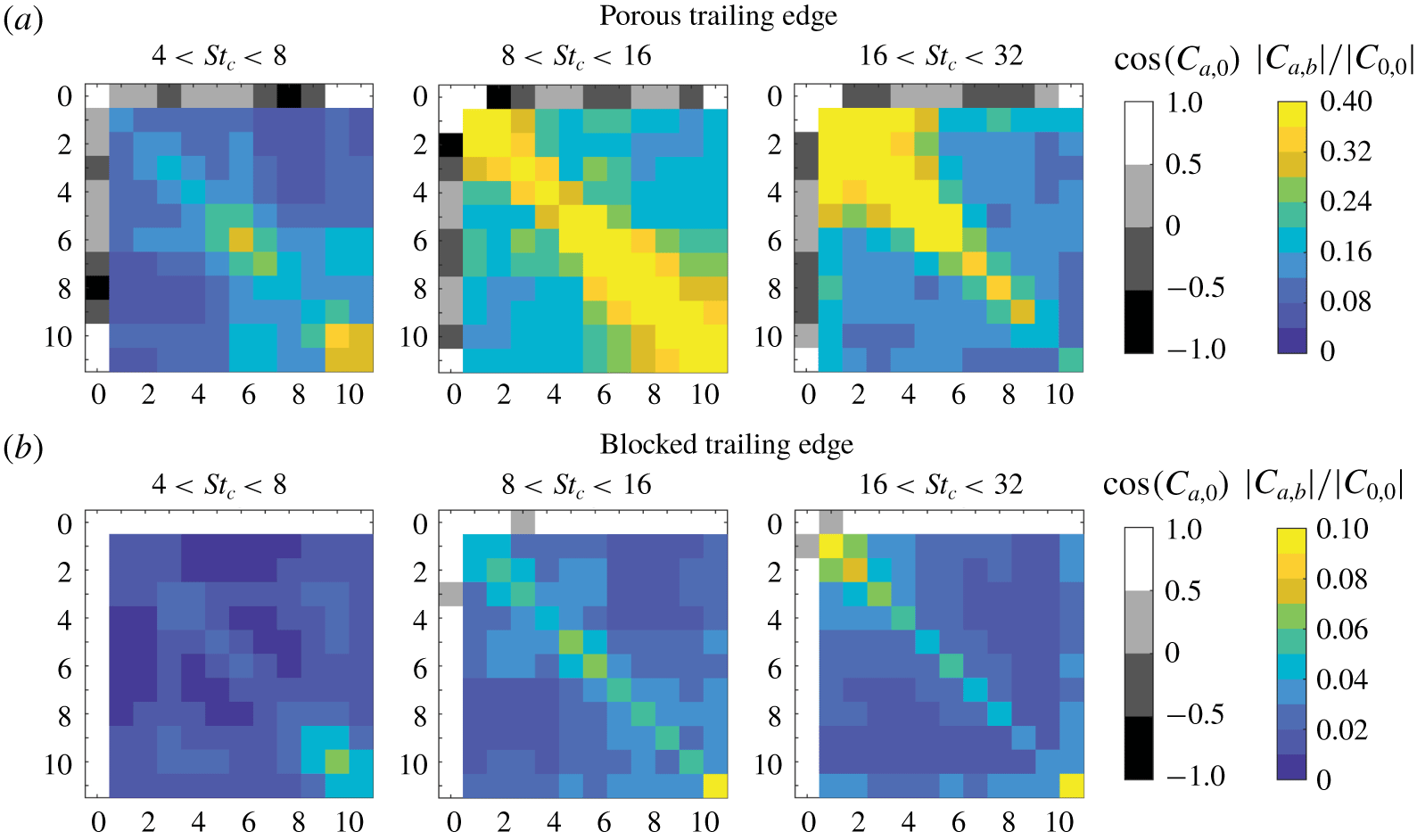
Figure 16. Normalized cross-spectral density (CSD) (inner coloured matrix) for the various strips and the resulting phase information (outer grey scale matrix) with respect to the overall trailing-edge region. Note that colour bars of (a) and (b) have different scales.
The phase-angle results are in line with the trends in figures 14 and 15. The strips of the porous TE show weaker in-phase relation than the blocked TE in addition to a number of strips with negative phase angles. Throughout the investigated frequency range, strips with the out-of-phase relation can be found just downstream of the solid–porous junction (i.e. strips 2 and 3), as well as at the middle segment of the trailing edge (i.e. from strips 6 to 9). These locations correspond to the strips that have large temporal lag in figure 15(b). Nonetheless, strip 1 and strip 11 consistently show positive  $\text{cos}(C_{a,0})$ values, which suggests a constructive interference between the sound sources at both the solid–porous junction and the actual trailing edge (Kisil & Ayton Reference Kisil and Ayton2018). On the other hand, none of the strips on the blocked TE shows an out-of-phase relation, which leads to the monotonic increase in the cumulative sum plots (figure 14). Hence, these findings further corroborate the argument that the porous TE promotes destructive interference among the distributed noise sources on the porous surface.
The CSD matrices provide additional insights into the acoustic source intensity of the porous and blocked TE. Note that the colour bars of figure 16(a,b) are presented with different ranges due to  $|C_{0,0}|$ (i.e. the total noise level of the 11 strips) of the blocked TE being significantly higher than that of the porous TE. For $4<St_{c}<8$, both porous and blocked TE exhibit a higher CSD magnitude towards the trailing edge, which implies that the scattering intensity surrounding the actual trailing edge for the porous TE case remains significant at low frequency. This is also evident in figure 14 where the slopes in between strips 10 and 11 of the porous TE are noticeably steeper compared to the others. For the frequency range of $8<St_{c}<16$, the CSD distribution for the porous TE becomes more uniform in the entire trailing-edge region. Conversely, the blocked TE shows the highest magnitude to be located on strip 11, which is in line with the location of the dominant noise source in the beamforming maps (figure 11). For $16<St_{c}<32$, porous TE shows a higher CSD level concentrated near the solid–porous junction, and the CSD decreases further downstream. High CSD magnitude surrounding the solid–porous junction can also be identified for the blocked TE, in addition to strip 11.
Based on the findings in this subsection, it is possible to argue that the noise reduction of the porous TE is a combination of two mechanisms. Firstly, the porous TE reduces the scattering intensity at the trailing edge. Secondly, the porous TE causes additional scattering at multiple streamwise locations along the porous surface, which results in destructive interference between scattered sound waves. Since these mechanisms are not observed in the blocked TE, they are considered to be driven by certain flow-field mechanism in the porous medium. To elucidate this matter, detailed flow-field analyses are presented in § 6.
6 Flow-field description
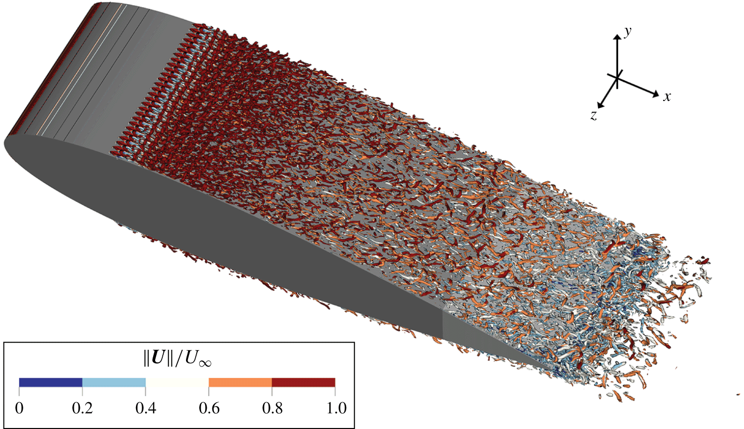
Figure 17. Instantaneous iso-surface of  $\unicode[STIX]{x1D706}_{2}=-1\times 10^{7}$ coloured with the contour of non-dimensional velocity magnitude $\Vert \boldsymbol{U}\Vert /U_{\infty }$ for the porous TE case. The porous medium is shaded in light grey.
The analyses in § 5 have confirmed that the permeability across the porous medium, which connects the flow field on the suction and pressure sides of the aerofoil, is essential for achieving noise reduction. Nevertheless, the presence of the porous medium might also alter the turbulence properties in the boundary layer near the trailing edge, which are also relevant to the trailing-edge noise generation mechanism. To obtain better insights into this matter, the effects of different trailing-edge treatments on the flow field are analysed in this section.
6.1 Flow organization in the turbulent boundary layer
Figure 17 shows  $\unicode[STIX]{x1D706}_{2}$ (Jeong & Hussain Reference Jeong and Hussain1995) iso-surfaces that depict the vortical structures caused by forced turbulent transition due to the zig-zag tripping device installed at $x/c=-0.8$. Furthermore, the iso-surface is coloured using the velocity magnitude $\Vert \boldsymbol{U}\Vert$ normalized with $U_{\infty }$. Streamwise vortices can be observed to form downstream of the tripping device, which evolve into hairpin-like structures (Elsinga & Westerweel Reference Elsinga and Westerweel2012). These flow structures gradually become more random as the boundary layer develops. Qualitatively, the discontinuity of surface boundary condition at the solid–porous junction does not appear to significantly alter the boundary-layer contents. Nevertheless, the flow characteristics nearby and inside the porous medium might differ in both porous and blocked TE cases due to the presence of the solid core in the latter. These aspects will be further discussed in the following.
6.2 Surface pressure fluctuation statistics
The presence of the porous trailing edge has been demonstrated to affect integral boundary-layer parameters (Geyer & Sarradj Reference Geyer and Sarradj2014; Rubio Carpio et al. Reference Rubio Carpio, Avallone, Ragni, Snellen and van der Zwaag2019b). Consequently, the surface pressure fluctuation statistics might also be altered, which in turn would influence trailing-edge noise radiation (Amiet Reference Amiet1976). Following this, the surface pressure fluctuation statistics are investigated in terms of autospectra and spanwise coherence length. These parameters have been chosen as they are relevant in the analytical formulation of broadband trailing-edge noise for solid surfaces, such as the model of Amiet (Amiet Reference Amiet1976; Roger & Moreau Reference Roger and Moreau2010).
Surface pressure fluctuation spectra  $\unicode[STIX]{x1D6F7}_{pp}$ at three different stations are plotted in figure 18. The locations are: $x/c=-0.23,-0.11,\text{and}-0.01$, which correspond to a position upstream of the solid–porous junction for both porous and blocked TE cases, half-way between the solid–porous junction and the trailing edge and near the trailing edge respectively. Figure 18(a) confirms that, upstream of the solid–porous junction, pressure fluctuations in the boundary layer are hardly affected by the different trailing-edge treatments, which is in line with the observation of Rubio Carpio et al. (Reference Rubio Carpio, Avallone, Ragni, Snellen and van der Zwaag2019b). At $x/c=-0.11$, $\unicode[STIX]{x1D6F7}_{pp}$ for both the porous and blocked TE increases above that of the solid TE, with the largest difference in the low frequency range ( $5<St_{c}<10$). Spectra over the solid TE are also compared with the Rozenberg, Robert & Moreau (Reference Rozenberg, Robert and Moreau2012) model using the boundary-layer parameters on the solid TE as the input. Good agreement is found at low frequencies up to $St_{c}=30$, while at higher frequencies, the slope of the numerical result is steeper than that of the Rozenberg model. Near the trailing edge, at $x/c=-0.01$, the $\unicode[STIX]{x1D6F7}_{pp}$ difference between the solid TE and porous TE becomes smaller, particularly at low frequency. Applying these trends to Amiet’s model would result in the noise intensity of the porous TE being similar, if not higher, than that of the solid TE. This contradicts the findings in § 5.
The spanwise coherence length is also a relevant parameter that is proportional to the far-field noise (Amiet Reference Amiet1976), i.e. reducing the spanwise coherence of the surface pressure fluctuations would also lead to noise reduction. The coherence length based on the surface pressure fluctuations  $l_{pp}^{z}(\unicode[STIX]{x1D714})$ is defined as the integral of the coherence function in the spanwise direction
 $$\begin{eqnarray}l_{pp}^{z}(\unicode[STIX]{x1D714})=\lim _{L\rightarrow \infty }\int _{0}^{L}\sqrt{\unicode[STIX]{x1D6FE}_{pp}^{2}(\unicode[STIX]{x1D714},\unicode[STIX]{x0394}z)}\,\text{d}\unicode[STIX]{x0394}z,\end{eqnarray}$$
 where  $\unicode[STIX]{x1D6FE}_{pp}^{2}$ is the magnitude-squared coherence between surface pressure fluctuations at two points along the spanwise ( $z$) direction and separated by $\unicode[STIX]{x0394}z$; $\unicode[STIX]{x1D6FE}^{2}$ is defined as follows:
 $$\begin{eqnarray}\unicode[STIX]{x1D6FE}^{2}(\unicode[STIX]{x1D714},\unicode[STIX]{x0394}z)=\frac{|C(\unicode[STIX]{x1D714},z_{1},z_{2})|^{2}}{|C(\unicode[STIX]{x1D714},z_{1},z_{1})||C(\unicode[STIX]{x1D714},z_{2},z_{2})|},\end{eqnarray}$$
 where  $C(\unicode[STIX]{x1D714},z_{1},z_{2})$ is the cross-power spectral density between the points at $z_{1}$ and $z_{2}$, which is defined in a similar manner as in (5.2); $\unicode[STIX]{x1D6FE}_{pp}^{2}$ is computed using a periodogram method with Hanning window and 50 % overlap, resulting in a frequency resolution of 100 Hz. However, due to a relatively short simulation time, additional procedures are employed to improve the convergence of the results. Firstly, the $\unicode[STIX]{x1D6FE}_{pp}^{2}$ is averaged along the aerofoil span in the range $-0.015<z/c<0.015$. Furthermore, a curve-fitting approach based on an exponential function is adopted to ensure that $\unicode[STIX]{x1D6FE}_{pp}^{2}$ is reduced to zero at large $\unicode[STIX]{x0394}z$. The exponential function is defined as follows (Palumbo Reference Palumbo2012; Van der Velden et al. Reference Van der Velden, Van Zuijlen, De Jong and Bijl2014):
 $$\begin{eqnarray}\unicode[STIX]{x1D6FE}(\unicode[STIX]{x1D714},\unicode[STIX]{x0394}z)_{pp}=\text{e}^{-|\unicode[STIX]{x0394}z|/l_{pp}^{z}(\unicode[STIX]{x1D714})}.\end{eqnarray}$$
 The coherence length  $l_{pp}^{z}$ plots at three different locations are shown in figure 19. The quantity has been normalized with the boundary-layer thickness at the trailing edge of the solid TE case ( $\unicode[STIX]{x1D6FF}_{99}$). Similarly to the surface pressure spectrum trends in figure 18, the coherence length of the three cases has a very similar level and slope at $x/c=-0.23$. Downstream of the solid–porous junction, at $x/c=-0.11$, the $l_{pp}^{z}$ of the solid TE increases above the level of both the porous and blocked TE cases, particularly in the low frequency range. Above $St_{c}=12$, however, all three cases become similar. This behaviour might be attributed to the enhanced turbulent mixing process near the porous medium surface as reported by Koh et al. (Reference Koh, Meinke and Schröder2018). At $x/c=-0.01$, $l_{pp}^{z}$ for all three cases shows almost a similar trend, although the coherence length for the solid TE is slightly higher at $St_{c}<8$. The $l_{pp}^{z}$ for the solid TE at the three stations are also compared with the Corcos (Corcos Reference Corcos1964) and Efimtsov (Efimtsov Reference Efimtsov1982; Palumbo Reference Palumbo2012) models using local flow-field information as input; the Corcos constant is equal to $1/2.1$ following Pröbsting, Tuinstra & Scarano (Reference Pröbsting, Tuinstra and Scarano2015) and Amiet (Reference Amiet1976). The trends from the simulations are generally in line with those of Efimtsov. The trend of the solid TE at $x/c=-0.01$ is also in good agreement with the Corcos model for $St_{c}>14$. Overall, the spanwise coherence length trends of the different trailing-edge treatments are of comparable magnitude, particularly near the solid–porous interface and the trailing edge. Therefore, it is unlikely that the minor alteration of $l_{pp}^{z}$ has an important role in noise abatement, at least in the present case.
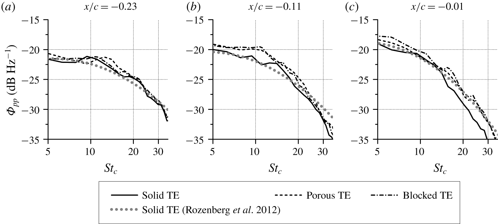
Figure 18. The comparison of power spectral density of surface pressure fluctuations  $\unicode[STIX]{x1D6F7}_{pp}$ between the three trailing-edge treatments. The value of $\unicode[STIX]{x1D6F7}_{pp}$ has been normalized with a reference pressure of 1 Pa. For comparison, the prediction of Rozenberg’s model (Rozenberg et al. Reference Rozenberg, Robert and Moreau2012) is included.
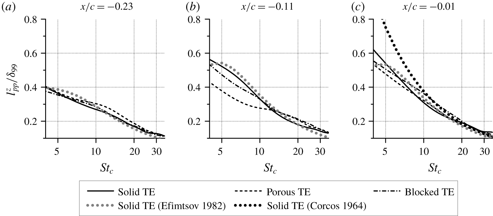
Figure 19. Spanwise coherence length ( $l_{pp}^{z}$) plotted against the chord-based Strouhal number ( $St_{c}$). For comparison, predictions of the Corcos (Corcos Reference Corcos1964) and Efimtsov models (Efimtsov Reference Efimtsov1982; Palumbo Reference Palumbo2012) are included.
This subsection has shown that the porous trailing edge affects flow-field statistics at the trailing-edge region. However, the observed trends do not fully correspond to noise attenuation according to the analytical TE noise model. It is also interesting to observe that the surface pressure statistics on both porous and blocked TE are rather similar despite the fact that only the former is able to attenuate noise. This further corroborates the argument that the noise prediction methods for solid aerofoils are not readily applicable to the porous ones (Geyer, Sarradj & Fritzsche Reference Geyer, Sarradj and Fritzsche2010; Rubio Carpio et al. Reference Rubio Carpio, Avallone, Ragni, Snellen and van der Zwaag2019b).
6.3 Near-field effects of the porous medium
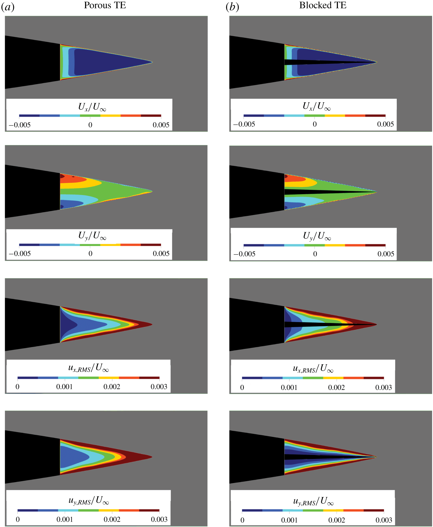
Figure 20. Contours of velocity statistics in the porous medium region of porous and blocked TE normalized with  $U_{\infty }$; the mean velocity components in the $x$ (
$x$ ( $U_{x}$) and $y$ directions ( $U_{y}$) are in the first and second rows respectively, and the corresponding root-mean-square of velocity fluctuations ( $u_{x,RMS}$ and $u_{y,RMS}$) are in the third and fourth rows respectively. Regions outside of the porous medium are masked in grey.
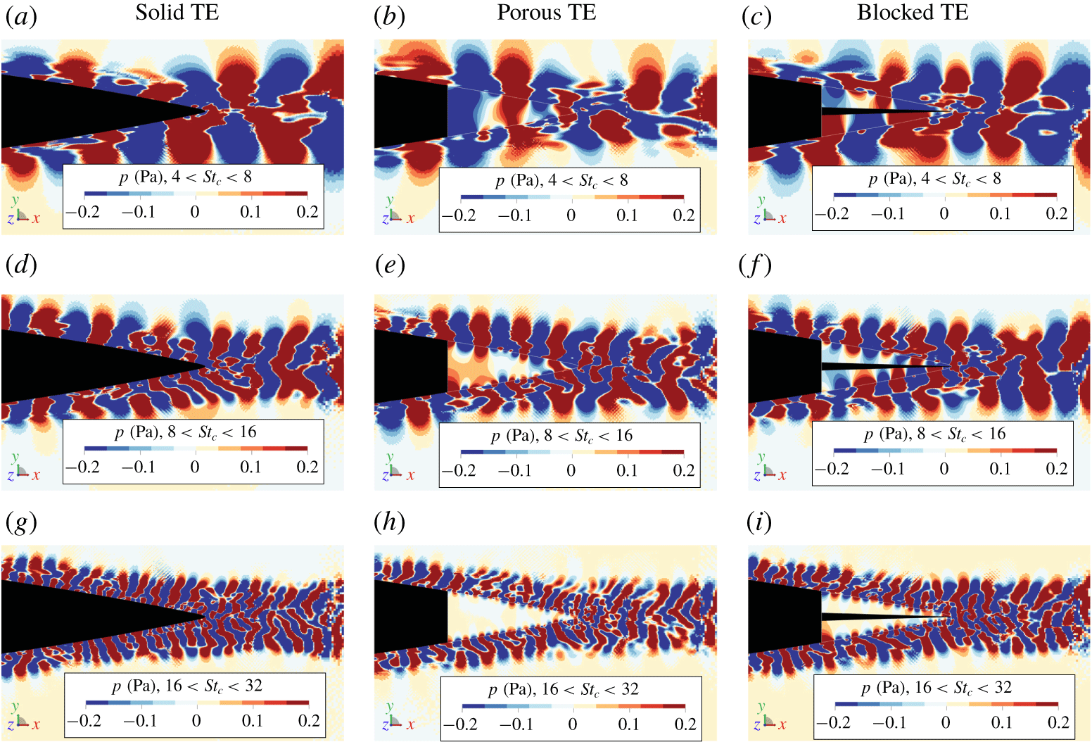
Figure 21. Instantaneous contours of band-passed pressure fluctuations ( $p$) at the mid-span of the three trailing-edge treatments in different frequency bands, i.e. $4<St_{c}<8$ in (a–c), $8<St_{c}<16$ in (d–f) and $16<St_{c}<32$ in (g–i).
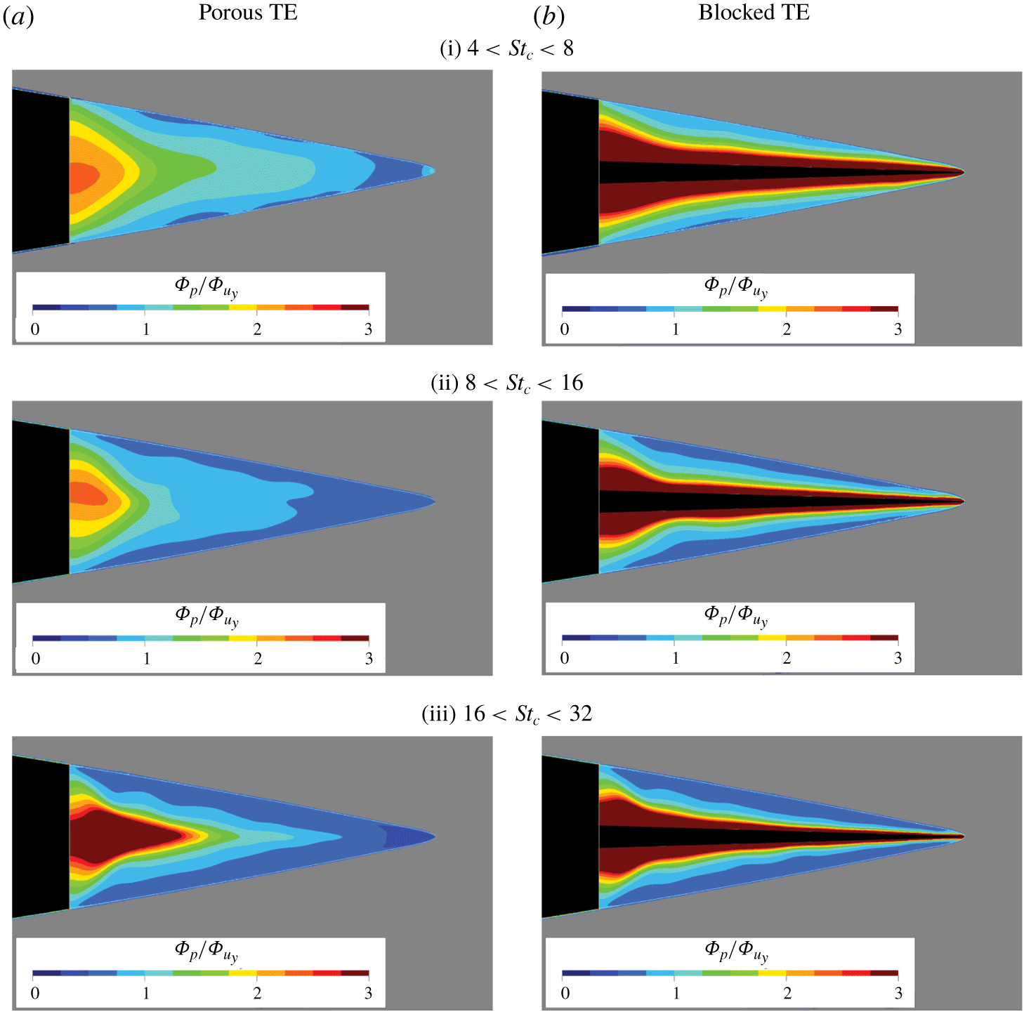
Figure 22. Contours of  $\unicode[STIX]{x1D6F7}_{p}/\unicode[STIX]{x1D6F7}_{u_{y}}$ inside the porous and blocked TE. The quantity has been normalized with $(U_{\infty }/(2q_{\infty }))^{2}$.

Figure 23. The chordwise variation of  $\unicode[STIX]{x1D6F7}_{p}/\unicode[STIX]{x1D6F7}_{u_{y}}$ along the chord line of the porous TE.
The previous subsection has shown that the alteration of surface pressure statistics in the boundary layer due to the porous TE cannot fully explain the resulting noise reduction. Instead, the noise reduction of the porous TE has been linked to the flow-field communication between the suction and pressure sides of the aerofoil (Rubio Carpio et al. Reference Rubio Carpio, Avallone and Ragni2018). To elucidate this behaviour, this subsection provides a detailed examination the flow field inside the porous medium for both porous and blocked TE cases.
The velocity field statistics inside the porous medium region of the porous and blocked TE are illustrated in figure 20. The figure shows that the mean  $x$-velocity component of both cases is dominated by regions with negative velocity. This indicates the presence of weak recirculation regions, similar to those observed in the porous flat plate of Showkat Ali et al. (Reference Showkat Ali, Azarpeyvand and Ilrio da Silva2018). Contours of the $y$-velocity component confirm that there is no mean cross-flow between both sides of the aerofoil due to the zero angle-of-attack setting. However, the contours of root-mean-square of velocity fluctuations show considerable differences between the porous and blocked TE. In both cases, the intensity of velocity fluctuations in the porous medium is relatively low (i.e. $O(10^{-2})$ of $U_{\infty }$). For the $u_{x,RMS}$ contour, the blocked TE shows a larger region with higher velocity fluctuations when compared to the porous TE, although $u_{x,RMS}$ in both cases tends to increase in the downstream direction where the flow resistance is lower due to smaller porous medium thickness (Bear Reference Bear1972; Naaktgeboren et al. Reference Naaktgeboren, Krueger and Lage2004). In contrast, $u_{y,RMS}$ of the blocked TE tends to zero towards the symmetry plane of the trailing edge due to the presence of the solid core. However, the contour for porous TE shows that $u_{y,RMS}$ gradually increases towards the downstream direction. Hence, based on figure 20, the noise reduction of the porous trailing edge is related to the unsteady flow fluctuations in the porous medium arising from the interaction between boundary layers on both sides of the aerofoil.
Contours of the band-passed spectra of the pressure fluctuations in figure 21 are plotted to corroborate the aforementioned argument. The porous TE allows turbulent fluctuations to permeate through the porous medium and to interact with those on the complementary side. However, this process becomes less prominent at higher frequency as smaller and milder fluctuations are dampened more efficiently by the porous medium. This behaviour is also reflected by the smaller slope of the cumulative sum of far-field noise contribution at high frequencies, as shown in figure 14. The contours of the blocked TE show that the solid core completely prevents the interaction between pressure fluctuations along the two sides of the aerofoil. Furthermore, it is also evident that the pressure fluctuation intensity in the boundary layer is weakly influenced by the porous medium, which is in line with the trends in figure 18. This might be the reason for the blocked TE to produce sound with a similar intensity as the solid TE, since the acoustic scattering on the blocked TE also takes place primarily at the trailing edge (see figures 11 and 16).
As described by Chase (Reference Chase1975), an impedance mismatch, such as the sudden transition from a solid surface to a free fluid at a trailing edge, induces the scattering of acoustic waves. Since the porous trailing edge can be considered as an intermediary surface condition that lies in between the impermeable solid and free fluid, it might be perceived by the incoming turbulent boundary layer as a region with spatially varying impedance, i.e. a continuous impedance mismatch. Such condition would allow the porous trailing edge to scatter noise at multiple locations from the solid–porous junction to the actual trailing edge (Kisil & Ayton Reference Kisil and Ayton2018), which is also reflected in figure 16. Conversely, it is implied that the solid core of the blocked TE would prevent the continuous variation of impedance, and thus acting as a solid TE.
To demonstrate the difference between the impedance distribution inside the porous medium regions of both the porous and blocked TE, the ratio between the power spectral density of pressure fluctuations and that of vertical velocity fluctuations  $\unicode[STIX]{x1D6F7}_{p}/\unicode[STIX]{x1D6F7}_{u_{y}}$ is computed and the resulting contours are plotted in figure 22. Additionally, $\unicode[STIX]{x1D6F7}_{p}/\unicode[STIX]{x1D6F7}_{u_{y}}$ along the chord line of the porous TE is plotted in figure 23. This quantity can be interpreted as the magnitude of the porous medium impedance (Kuczmarski & Johnston Reference Kuczmarski and Johnston2011; Koh et al. Reference Koh, Meinke and Schröder2018). Overall, the figure shows that the impedance inside the porous TE generally decreases in the streamwise direction, for any given frequency range. The plots in figure 22 illustrate that the trends at $4<St_{c}<8$ and $8<St_{c}<16$ are relatively similar near the solid–porous junction, but further downstream, the latter decreases at a faster rate. There is a noticeable peak nearby the trailing edge for $4<St_{c}<8$ which implies a significant scattering at this location, as previously indicated in figure 16. Near the solid–porous junction, $\unicode[STIX]{x1D6F7}_{p}/\unicode[STIX]{x1D6F7}_{u_{y}}$ at $16<St_{c}<32$ is shown to be significantly higher than at other frequencies. This is likely to be due to the lower velocity fluctuations in the porous medium at high frequency, as depicted in figure 20. The large $\unicode[STIX]{x1D6F7}_{p}/\unicode[STIX]{x1D6F7}_{u_{y}}$ gradient in this frequency range might also be responsible for the concentrated acoustic scattering surrounding the solid–porous junction, which is in line with figure 16. In contrast to the porous TE, the blocked TE contours show similar trends for all three frequency bands. These behaviours can be associated with the $u_{y,RMS}$ contours in figure 20; the $u_{y}$ along the symmetry plane of the porous TE remains finite whereas that of the blocked TE reduces to zero next to the solid core. As a result, the impedance in the blocked TE approaches infinity, similar to that on the solid TE surface. On the other hand, the smaller $\unicode[STIX]{x1D6F7}_{p}/\unicode[STIX]{x1D6F7}_{u_{y}}$ at the trailing edge of the porous TE would realize a milder impedance jump, and in turn, lower trailing-edge scattering efficiency (Rubio Carpio et al. Reference Rubio Carpio, Avallone and Ragni2018, Reference Rubio Carpio, Avallone, Ragni, Snellen and van der Zwaag2019b). This is also reflected by the difference in the dominant source location between the porous and blocked TE in the beamforming maps (see figure 11).
6.4 Aerodynamic performance
The use of the porous trailing edge has been reported to adversely affect aerodynamic performance of the aerofoil, such as increased drag (Wilkinson Reference Wilkinson1983; Jimenez et al. Reference Jimenez, Uhlmann, Pinelli and Kawahara2001; Herr et al. Reference Herr, Rossignol, Delfs, Lippitz and Mner2014) and reduced lift (Geyer & Sarradj Reference Geyer and Sarradj2014). Hence, the effect of the porous trailing edge on the aerodynamic performance is investigated in this subsection. The time-average drag coefficient has been estimated by measuring the total pressure deficit in the aerofoil wake, following Schlichting & Gersten (Reference Schlichting and Gersten2016), as shown in (6.4).
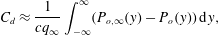 $$\begin{eqnarray}C_{d}\approx \frac{1}{cq_{\infty }}\int _{-\infty }^{\infty }(P_{o,\infty }(y)-P_{o}(y))\,\text{d}y,\end{eqnarray}$$
 where  $q_{\infty }$ is the mean free-stream dynamic pressure and $P_{o}$ is the time-averaged total pressure. The total pressure is measured at the aerofoil mid-span, along $-2.5<y/c<2.5$ at $x/c=4$. The time history of the total pressure at each measurement point has been averaged over a period of 10 flow passes.
Table 3. The drag coefficient estimate for the different trailing-edge treatments, and the corresponding relative difference from the solid TE.
The drag coefficient estimates are shown in table 3. Both porous and blocked TE show increased drag compared to the solid TE, consistent with previous experimental observations (Flack & Schultz Reference Flack and Schultz2014; Rubio Carpio et al. Reference Rubio Carpio, Avallone, Ragni, Snellen and van der Zwaag2019a). Since the simulation does not consider the surface roughness contribution, the drag increase is mainly due to a higher wall shear stress due to the permeability of the porous medium (Jimenez et al. Reference Jimenez, Uhlmann, Pinelli and Kawahara2001), which is also evident in the mean wall-friction coefficient  $C_{f}$ as shown in figure 24. Interestingly, the $C_{f}$ of the porous trailing edges also decreases slightly just downstream of the solid–porous junction ( $x/c=-0.2$), which has also been reported by Koh et al. (Reference Koh, Meinke and Schröder2018).

Figure 24. Streamwise distribution of mean wall-friction coefficient  $C_{f}$ for the different trailing-edge cases.
7 Conclusion and outlook
This manuscript has presented a study on the turbulent boundary-layer trailing-edge noise generation from a NACA 0018 aerofoil with and without a porous trailing edge. The flow field is resolved using the transient, explicit and compressible lattice-Boltzmann solver, PowerFLOW. The aerofoil is set to zero angle of attack and the porous treatments are applied at the last 20 % of the aerofoil chord. The properties of the porous medium is modelled using an equivalent fluid region governed by Darcy’s law, in which the porosity and flow resistivity corresponding to a metal foam have been applied. In addition to the solid TE and the porous TE, a third configuration was considered by adding a thin solid core at the symmetry plane of the porous trailing edge (i.e. blocked TE). Simulation results are validated against experimental data. Boundary-layer parameters and far-field sound characteristics were found to be in good agreement against past experiments. Compared to the solid trailing edge, the porous TE reduces noise by up to 9 dB in low frequency range whereas the blocked TE fails to produce such benefit. Subsequently, the locations of dominant sound sources on each trailing-edge variant are obtained using the conventional beamforming technique. The maximum noise source intensity is found at the actual trailing edge for both solid and blocked TE, and near the solid–porous junction for the porous TE. This finding is also in line with other experimental works.
In order to elucidate the acoustic scattering behaviour of the porous trailing edge, the trailing-edge region was segmented into chordwise strips. Subsequently, the far-field noise contribution from the strips and their phase relations were evaluated. The results suggested that sound sources are distributed along the surface of porous TE, whereas for blocked TE, they are mainly concentrated at the trailing edge, similar to solid TE. These findings also imply that the porous TE behaves as continuous trailing edges with acoustic scattering at multiple locations as a consequence (Kisil & Ayton Reference Kisil and Ayton2018). Flow-field measurements are performed to determine whether the noise reduction of the porous TE can be attributed to flow-field alterations. Subsequently, surface pressure fluctuation spectra and spanwise coherence length are investigated as these are relevant parameters in conventional trailing-edge noise models, such as that of Amiet (Reference Amiet1976). It is found that the surface pressure statistics upstream of the solid–porous junction are similar among all three types of trailing edge. Nevertheless, downstream of the solid–porous junction, both blocked and porous TE exhibit slightly stronger surface pressure fluctuations, while the spanwise coherence length was slightly lower when compared with the solid counterpart. However, these are found to be insufficient to fully explain the noise reduction of the porous TE.
It is also found that the mean velocity components inside both porous and blocked TE are similar. However, the contours of velocity fluctuations are different, particularly for the vertical component; the porous TE showed a finite velocity fluctuations that gradually increased towards the trailing edge, while the blocked TE showed velocity fluctuations that tended towards zero along the chord line due to the solid core. The near-field pressure fluctuations were also examined, and they revealed that the surface pressure fluctuations were not significantly affected by the presence of the porous medium. The spatial variation of flow impedance in the porous medium is also examined. The impedance of the porous TE gradually decreases towards the trailing edge, resulting in milder impedance discontinuity at the trailing edge. Moreover, following Chase (Reference Chase1975) and Kisil & Ayton (Reference Kisil and Ayton2018), the spatially varying impedance in the porous TE is responsible for acoustic scattering at multiple streamwise locations. Conversely, the impedance variation was not found in the blocked TE, and consequently, the impedance discontinuity at the trailing edge remains large, leading to intense scattering that is similar to the solid TE case.
To conclude, this manuscript has identified two noise reduction mechanisms of an open-cell metal-foam porous trailing edge: (i) the reduced scattering intensity at the trailing edge due to the milder impedance mismatch at this location, and (ii) the destructive interference between acoustic waves that are scattered from different locations along the porous medium surface due to the continuous impedance variation. Both mechanisms are driven by the unsteady flow-field interaction across the porous trailing edge. This hints at a possibility to optimize the streamwise distribution of permeability in order to further increase the noise reduction capability, e.g. by minimizing the impedance jump at the solid–porous junction (Delfs et al. Reference Delfs, Faßmann, Lippitz, Lummer, Mößner, Müller, Rurkowska and Uphoff2014). Furthermore, as computational cost becomes more affordable, it would be feasible to perform a simulation that considers the internal topology of the porous material without requiring any porous medium model. Such investigation would provide further insights into the underlying physical mechanisms that have been pointed out in this manuscript.
Acknowledgements
The authors would like to acknowledge the technical support of Dr W. van der Welden from Dassault Systemes regarding the PowerFLOW template for the aerofoil trailing-edge noise study. The authors also would like to thank colleagues at the Delft University of Technology: S. Luesutthiviboon for his suggestion regarding the design and optimization of the beamforming array used in the present study, and A. Rubio Carpio for providing additional insights on the interpretation of simulation results based on the experimental observations. This study is supported by the project SMARTANSWER (Smart Mitigation of flow-induced Acoustic Radiation and Transmission for reduced Aircraft, surface traNSport, Workplaces and wind enERgy noise) which has received funding from the European Union’s Horizon 2020 research and innovation program under the Marie Skodowska-Curie grant agreement no. 722401. More information can be found on https://www.h2020-smartanswer.eu/.
Declaration of interests
The authors report no conflict of interest.


 Open access