


1. Introduction
Large areas of the arctic and sub-arctic environments are covered by lakes and rivers (e.g. >30% of the Lena Delta in northern Siberia (Reference Schneider, Grosse and WagnerSchneider and others, 2009) and 15–40% of North America (Reference Duguay, Flato, Jeffries, Ménard, Rouse and MorrisDuguay and others, 2003)). With melt onset and ice decay, the lake ecosystem underlies dramatic changes. Thermal- and wind-driven mixing of the water column starts, the albedo and heat fluxes change, evaporation and the exchange of further gases increase. The surrounding areas are also affected, because of the thermal moderation effect of water bodies.
Changes in the timing of lake- and river-ice decay are indicators for climatic change (Reference Johnson and StefanJohnson and Stefan, 2006), as ice growth and decay are directly controlled by atmospheric fluxes (Reference Prowse, Bonsal, Duguay and LacroixProwse and others, 2007). For instance, earlier thaw dates would lead to earlier starts of greenhouse-gas exchange and to higher evaporation rates from the water surfaces in early summer.
Satellite-borne synthetic aperture radar (SAR) is a suitable tool for observing ice decay, as the backscattered signal from the surface to the radar is highly dependent on the dielectric properties and the structure of the surface and subsurface layers. As the dielectric constants and losses of water and ice are very different, their backscattering signature can be easily distinguished in many cases. The satellite signal penetrates the cloud cover and can be used to monitor vast uninhabited regions, such as the Arctic tundra, cost-efficiently and in near-real time. Threshold-based methods, change detection techniques in time series and manual mapping are methods commonly used to monitor ice decay from SAR images (e.g. Reference Jeffries, Morris, Weeks and WakabayashiJeffries and others, 1994; Reference Geldsetzer, Van der Sanden and BriscoGeldsetzer and others, 2010). As the backscatter of ice or water is dependent on the radar wavelength, polarization and incidence angle (Reference Wakabayashi, Weeks and JeffriesWakabayashi and others, 1993; Reference Mäkynen, Manninen, Simila, Karvonen and HallikainenMäkynen and others, 2002) the threshold for dividing ice and water needs to be matched to the radar configuration. Change detection requires time series of images taken with identical sensors and identical imaging geometries. For monitoring at a very high spatial (down to a few meters pixel size) and temporal (weekly to daily) resolution, the repeat pass time of recent satellite missions is often not high enough. Mapping based on visual analyses by an experienced operator is sensor-independent, and relatively robust to errors due to misclassifications, but time-consuming. A robust and time-saving method independent of sensor configuration is not yet available.
One option for automated image segmentation is clustering methods. The most common clustering method is the unsupervised k-means classification algorithm. The details of the algorithm are given by Reference Tou and GonzálesTou and Gonzáles (1974). This algorithm is implemented in most image-processing software packages. The advantage of unsupervised methods, such as k-means clustering, is that they require no prior training. The data points are partitioned to a defined number of clusters using the minimum distance technique (Reference Coleman and AndrewsColeman and Andrews, 1979; Reference Jain, Murty and FlynnJain and others, 1999).
The preparation of data prior to clustering influences the classification results. Filters are often applied to the data prior to image classification to suppress speckle (Reference DengDeng, 2005; Reference Geldsetzer, Van der Sanden and BriscoGeldsetzer and others, 2010). The choice of the filter type and filter size thus has a strong impact on the results. The subsequent application of morphological filters can correct small misclassifications. The morphological closing filter has been applied successfully in several studies (e.g. Reference Wesche and DierkingWesche and Dierking, 2012).
The aim of this study is to analyze the performance of the unsupervised k-means classification method for estimating lake- and river-ice decay from SAR observations. The algorithm was tested with TerraSAR-X images for lakes and applied on RADARSAT-2 data for several lakes and river channels located in the central part of the Lena Delta. The effect of low-pass filtering of the data prior to classification and of the morphological closing filter on the classification results was also investigated. The outcome was compared to corresponding results derived with the commonly used threshold method and hand-mapped references. Lakes and rivers were treated separately in this study, as ice conditions on the river channels differed from those on the lakes.
2. Material and Methods
2.1. Study area
The lakes and river sections analyzed in this study are located in the southern central part of the Lena River Delta, northern Siberia, Russia, at 72° N, 126° E (Fig. 1). The area is a polygonal Arctic tundra landscape, located in a zone of continuous permafrost and covered by several ponds, lakes (with areas from 15 m2 to 1.7 km2) and river channels. The mean annual air temperature is –13.6°C, with monthly mean temperatures of around –35°C in winter and up to 13.4°C in summer. The average annual precipitation is 263 mm. Snow depth is 13–24 cm on average, but highly variable between the years and across the landscape because of redistribution through strong winds (Reference Boike, Wille and AbnizovaBoike and others, 2008). The polar night lasts from 15 November to 28 January and the polar day from 7 May to 7 August. Lake-ice decay commonly starts at the end of May and lasts until the end of June. River-ice break-up commonly occurs at the end of May or early in June (personal communication from J. Boike and others, 2010).
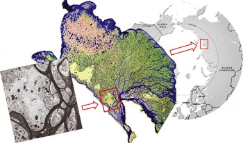
Fig. 1. Location of the area investigated. Left: RADARSAT-2 image (Canadian Space Agency, 2011); middle: Landsat-7 Enhanced Thematic Mapper Plus (ETM+) mosaic (NASA 2000/01); right: circum-Arctic map (Hugo Ahlenius, United Nations Environment Programme/Global Resources Information Database (UNEP/GRID)-Arendal 2008).
2.2. Data
All images were acquired on the ascending orbit. TerraSAR-X operates at X-band, i.e. at a frequency of 9.6 GHz (wavelength 3.1 cm), and RADARSAT-2 operates at C-band (5.4 GHz, 5.6 cm). The polarization of the TerraSAR-X images is HH (i.e. the transmitted and received signal are horizontally polarized); the RADARSAT-2 images are in Quad-Pol mode, i.e. polarizations HH, HV, VH and VV are measured simultaneously (V: vertically polarized). Additional information is given in Table 1. Our time series covers the whole spring period, from the end of April to the end of June, at the highest possible temporal resolution, considering that similar imaging geometries are required.
Table 1. Characteristics of the TerraSAR-X (TSX) and RADARSAT-2 (RS-2) images
2.3. Methods
Six TerraSAR-X and three RADARSAT-2 images (all originally in SLC (single look complex) format) were analyzed for this study. The SARScape and ENVI software packages were used for image processing and further image analyses. The images were radiometrically calibrated, normalized and geocoded (WGS84, UTM 52N). After geocoding, the pixel size of the TerraSAR-X images was 3.74 m × 3.74 m and that of the RADARSAT-2 data was 10.96m × 10.96 m. The output is given in terms of the radar backscattering coefficient, σ 0. A Lee filter (Reference LeeLee, 1980) with a kernel size of 3 × 3 was applied to the geocoded data to reduce speckle. Following this basic data processing, different methods were applied to determine which processing chain delivers the best results for separating ice and water surfaces. An overview of the different processing chains is given in Figure 2.
Fig. 2. Workflow description for (a) lakes and (b) rivers.
As shown in the figure, a low-pass filter (kernel size 3 × 3) was used in addition in one of the processing chains. Each center pixel value is replaced with an average of the surrounding values. This filter suppresses high-frequency variations in the data, which reduces strong intensity outliers, but also blurs natural sharp backscatter variations, as they occur (e.g. at ice/water edges).
In the next step, regions of interest (ROIs) were defined, covering lake surfaces and river sections. For classification into ice and water fractions, each ROI was treated separately. All pixels outside a ROI were masked out, leaving only pixels inside the ROI for further analysis.
An unsupervised k-means classification was applied to the remaining data. With this method, the image intensity values are partitioned into k classes in which each intensity value belongs to the class with the nearest mean. For the approach of dividing lake or river surfaces into ice and water areas, the number of classes was set to two. The initial clusters are randomly chosen. Then the class members are adjusted in an iterative refinement approach until the sum of all distances between the intensity value and the mean is as small as possible for both clusters (minimum-distance technique). Five iterations were allowed for reclassification of the pixels.
The closing filter, a morphological filter, was applied to the classification results. This filter eliminates small holes, and fills gaps which are smaller than the structural element of the surrounding pixels (Reference Haralick, Sternberg and ZhuangHaralick and others, 1987).
The outputs are the areas of the water and ice fractions, given by the number of pixels. The spatial pattern of the classes can be displayed.
To estimate the performance of the k-means classification in comparison with the threshold method, the performance of the latter was also tested for all investigated lake surfaces. To determine the threshold value for the TerraSAR-X images, the mean backscatter value and the standard deviation of the ice surfaces of seven randomly chosen lakes were calculated. Then the threshold, τσ, was fixed by
where
![]() is the mean ice-surface backscatter of all statistically investigated lakes and s is the mean standard deviation of σ. Here, τa
is –17.58dB for the TerraSAR-X HH-polarized data. This threshold was applied to all lakes during the entire thaw period. Pixels containing values <τa
were classified as water, those with >τa
as ice. The slightly varying incidence angles of the different acquisition dates were not taken into account, as the backscatter difference caused by the change in the incidence angle lies within the range of the standard deviation, s = 3.62 dB. This is in agreement with Reference Wakabayashi, Weeks and JeffriesWakabayashi and others (1993), who modeled an incident-angle-dependent backscatter change of 1 dB between 30° and 40° (C-band, VV polarization) for floating lake ice, and with Reference Mäkynen, Manninen, Simila, Karvonen and HallikainenMäkynen and others (2002), who measured the same backscatter shift on deformed sea ice. For the RADARSAT-2 data we used threshold values of –21.35 dB for HH-polarized and –24.35 dB for HV-polarized data, as determined by Reference Geldsetzer, Van der Sanden and BriscoGeldsetzer and others (2010).
is the mean ice-surface backscatter of all statistically investigated lakes and s is the mean standard deviation of σ. Here, τa
is –17.58dB for the TerraSAR-X HH-polarized data. This threshold was applied to all lakes during the entire thaw period. Pixels containing values <τa
were classified as water, those with >τa
as ice. The slightly varying incidence angles of the different acquisition dates were not taken into account, as the backscatter difference caused by the change in the incidence angle lies within the range of the standard deviation, s = 3.62 dB. This is in agreement with Reference Wakabayashi, Weeks and JeffriesWakabayashi and others (1993), who modeled an incident-angle-dependent backscatter change of 1 dB between 30° and 40° (C-band, VV polarization) for floating lake ice, and with Reference Mäkynen, Manninen, Simila, Karvonen and HallikainenMäkynen and others (2002), who measured the same backscatter shift on deformed sea ice. For the RADARSAT-2 data we used threshold values of –21.35 dB for HH-polarized and –24.35 dB for HV-polarized data, as determined by Reference Geldsetzer, Van der Sanden and BriscoGeldsetzer and others (2010).
No ancillary data were available to quantify the accuracy of either method and the influence of the different filters. Therefore, ice areas on the lakes were mapped by an experienced operator for 30 cases (described in detail in Section 3.1), chosen from the TerraSAR-X data. Under calm wind conditions, ice appears brighter than water in the radar images. However, at higher wind velocities the water also appears bright, because its rougher surface due to waves causes enhanced backscattering. The higher brightness of wind-influenced water makes it difficult to distinguish water from ice. Polygons including the ice surface were drawn carefully along the ice/water edges for each case separately.
Finally, we tested whether the k-means classification is a suitable tool for partitioning ice and water on river channels. The workflow is the same as for lake surfaces (with the steps listed in Fig. 2b).
3. Results
3.1. Lakes
Fourteen lakes were analyzed to evaluate the different methods: two lakes were analyzed at four different dates (four different stages of lake-ice melt); three lakes at three dates; four lakes at two dates; and five lakes at one date. Thus, a total of 30 cases were investigated (as described in Section 2.3), all with TerraSAR-X data. Some examples of the performance of each method and ice-cover fractions ranging from 88% to 27% are shown in Figure 3.

Fig. 3. TerraSAR-X subsets of six lakes taken on 16 June 2011. The classification results show the water surfaces in black and the ice surfaces in white. The percentages quantify the fraction of the ice class. Threshold is –17.58 dB. C is closing filter and L is low-pass filter.
To evaluate the accuracy of the different methods, the classification error was calculated in comparison to the manually derived reference for each case and method separately. The box plots in Figure 4 show the overall performance of the different methods compared to the reference. The values are also given in Table 2. The reasons for the statistical outliers are discussed in Sections 4.1 and 4.3.
Fig. 4. Error of the different classification methods compared to the reference for the TerraSAR-X data. C is closing filter, L is low-pass filter.
Table 2. Statistical performance of the different methods on the TerraSAR-X data. The error is given as the percentage difference between the methods and the reference for all 30 cases
3.1.1. Application to RADARSAT-2 data
The k-means classification algorithm was then applied on C-band Quad-Pol RADARSAT-2 data. The classification was carried out separately for each image. Again, the results were compared to references and the threshold method. The results of the HV- and the VH-polarized images were the same, but they differed slightly between the HH- and VV-data. We did not test the performance of the threshold method on the VV-polarized data, as no threshold value for this data is given by Reference Geldsetzer, Van der Sanden and BriscoGeldsetzer and others (2010). As our RADARSAT-2 data captured only this one partly ice-covered lake (all other lakes were ice-free during image acquisition), the data were not suitable for estimating a reasonable threshold value. The classification results of one lake recorded at the different polarizations are shown in Figure 5.

Fig. 5. Results of the application of k-means classification and filtering, and the threshold method on RADARSAT-2 data from 26 June 2011. C is closing filter, L is low-pass filter.
3.2. Rivers
To determine the ice and water fractions of river channels, 25 ROIs were set to analyze different parts of the river in the TerraSAR-X and RADARSAT-2 images. In two of the available TerraSAR-X images (acquired 25 and 30 May 2011) and in one RADARSAT-2 image (acquired 2 June 2011), fractions of ice and water were observed in the river channels. Again, the classification was performed on images which were low-pass-filtered to analyze the effect of the filter on the classification results (Fig. 2b).
As the ice cover on the river was broken into several smaller floes, it was not possible to mark all ice fragments by ROIs. Instead, we visually compared the classification results, focusing on the pattern of the spatial distribution of the ice and water surfaces. The pattern of the ice and water distribution in the classification results is in good agreement with the observations from the SAR images, even though the backscatter of the ice surface is more variable on the river channels than on the lakes. This results in comparatively less pronounced backscatter differences between the ice and the water surfaces, which may cause problems in the clustering via the minimum-distance technique. One example of the patterns of the backscatter in the X- and C-band SAR images and the corresponding classification results is shown in Figure 6.

Fig. 6. Separation of water (blue) and ice (white) surfaces in a river channel northeast of Samoylov Island with the k-means classification algorithm. L is low-pass filter. Dates are day/month/year.
On 25 May 2011, the ice surface was very wet, as the air temperatures rose above 0°C in the days before image acquisition and snowmelt had started (Reference Sobiech, Boike and DierkingSobiech and others, 2012). Therefore, the backscatter intensity of the ice was low and close to the backscatter values of the water. This leads to misclassifications of the wetter parts of the ice-covered areas. Before the acquisition of the next image (30 May 2011) in the time series, the main river-ice break-up occurred, completely changing the ice-cover characteristics. The ice then consisted of several ice sheets with different properties which were pushed together during break-up, remaining in place after the peak of the flood. Some parts of the ice sheets which appear dark in the radar image were misclassified as water, whereas the ice sheets appearing lighter were fully classified as ice.
The acquisition of the image on 2 June 2011 was carried out with the RADARSAT-2 sensor, delivering data in all polarizations. As HV and VH have the same properties, the VH data are not shown here. The ice conditions were the same as described for the former image. The results show that the classification performed best with HH-polarized input data. In case of cross-polarized data, the ice surface is underestimated. VV-polarized images are more sensitive to wind effects on the water surface (Section 4.5), so the water area marked in Figure 6 is partly misclassified as ice. The ice sheets which appear dark in the radar image are also partly misclassified as water, which makes the image recorded with VV-polarization the least suitable choice for automatic image classification.
The application of the low-pass filter before image classification improves the results. The water surfaces, especially, are classified with a higher accuracy. The closing filter should not be applied to the classification results, as the natural backscatter variations on river sections are high. Small gaps between the ice floes would be misclassified as ice, and the number of misclassified water pixels would rise.
4. Discussion
Sections 4.1–4.5 refer to lakes only. The results of the k-means classification on river channels are discussed separately, in Section 4.6.
4.1. Low-pass filtering
The low-pass filter smooths the image as it replaces the center pixel values with an average of the surrounding values. The advantage is that intensity outliers are suppressed. The disadvantage is that the edges of the lakes and the ice/water transitions are blurred (as mentioned in Section 2.3). Our results show that the majority of the pixels are better classified after application of this filter, but the ice pixels along the ice/water boundary are often misclassified as water. Thus the filter can be recommended if the overall result is of interest, but should not be applied if the correct ice/water edge is essential.
The filter worsens the results when the ice surface is wet and many pixels representing the ice surface have relatively low backscatter values (e.g. if melt ponds are present). In this case, the backscatter value of the pixels surrounding the melt ponds is lowered and consequently later misclassified as water.
4.2. k-means classification vs threshold method
The methods are both based on the backscatter differences of the signal from ice and water surfaces. The backscatter received by the sensor is usually higher from an ice surface than from a water surface, due to the different dielectric and surface properties of water and ice and due to scattering contributions from the ice volume. The absolute backscatter values also depend on the radar wavelength, polarization and incidence angle (Section 1).
To determine the threshold value for allocation of the pixels to either the ice or the water class, some statistics need to be performed first. The usual way to obtain the threshold is to investigate the mean backscatter values and standard deviations of some randomly chosen ice surfaces. Reference Geldsetzer, Van der Sanden and BriscoGeldsetzer and others (2010) took the lowest mean ice backscatter value from a number of different lakes minus the standard deviation as the threshold value for C-band HH-polarized data. In the present study, some of the lakes were covered by ice with a very wet surface, leading to very low backscatter values compared to typical values for ice. Taking this value minus the standard deviation would lead to such a low threshold value that the water surfaces would be greatly overestimated. Thus, the mean backscattering value of all statistically investigated ice surfaces minus the standard deviation was used in this study for the TerraSAR-X data (as described in Section 2.3). The general problem with the threshold method is that a new threshold has to be defined for each radar wavelength, polarization and incidence angle, and also for different ice and meteorological conditions. This implies that either statistics need to be performed for each new condition, or that a relatively large error occurs under changing conditions. In this study, we tested the performance of one carefully estimated threshold value on TerraSAR-X data acquired on different dates and slightly varying incidence angles (Table 1).
The advantage of an unsupervised classification method, such as k-means, is that the algorithm itself sets the limits of the backscattering intensity intervals for pixel allocation to classes, i.e. the threshold between ice and water. Therefore, the absolute values of the backscattering coefficients are not important. The simple fact that the sigma values from ice and water surfaces are significantly different is used. It is not necessary to first perform statistical analysis of the backscatter values to determine a threshold. In addition, the k-means algorithm is flexible to the ice conditions during image acquisition.
The unsupervised k-means classification algorithm is implemented in most image-processing software packages. The user defines the ROI and the number of classes, but the recording conditions of the input images do not have to be taken into account. As the image processing from each sensor and image can be the same for this approach, the image-processing chain can be automated easily, saving time and manpower.
The results of the performance of the unsupervised k-means classification are comparable to those of the threshold method (Fig. 4; Table 2). The mean values are almost the same. The median is slightly better for the threshold method than for the k-means method, but the 75% quartile value, as well as the maximum error, are reasonably lower for k-means than for the threshold method.
Taking into account that the k-means classification approach does not require any prior data analysis, thus saving a large amount of time compared to the threshold method, and that this approach adapts itself to new image-recording conditions and natural conditions, the k-means approach is superior to the threshold method. However, the k-means classification is only suitable when water and ice fractions are present. To determine the onset of ice breakup from a time series, other methods (e.g. visual image inspection, change detection or thresholding) are needed.
4.3. Application of the closing filter
Usually the lake ice melts from the shore to the inner part of the lake. If so, the ice surface is continuous and the closing filter reduces misclassifications due to speckle or wet ice patches and helps to display the natural conditions.
As shown in Figure 4, the closing filter has good overall performance and strongly enhances the results in most cases. However, the application of the closing filter can, in some cases, worsen the results, leading to the outliers shown in Figure 4. These outliers occur if the water surface is rough, leading to a large number of misclassified pixels in the water area. The closing filter then connects the misclassified pixels. The result is that most of the water surface is wrongly classified as ice. Since X-band data are more sensitive to wind speed and direction than images acquired at lower frequencies (Reference Long, Collyer and ArnoldLong and others, 1996), this problem is less critical at C-band. These outliers are easy to identify through a quick comparison of the original SAR image and the classification results by an operator. Thus our suggestion is to apply the closing filter in general, as it usually improves the results, but to perform a quality check.
4.4. Lake size
The lake size does not seem to be important for the performance of any method. The smallest lake analyzed in this study has a size of 0.049 km2, the largest an area of 1.729 km2. No connection was found between classification error and lake size. However, all lakes analyzed in this study are typical High Arctic polygonal tundra lakes, which are rather small and usually have a uniform ice cover. Larger lakes may have a less uniform ice cover, which would make the classification more difficult.
4.5. Wind
In former descriptions of the separation of lake ice and water in SAR images, the wind velocity was used as a criterion to decide whether it is possible to automatically classify the surfaces into ice and water (Reference Geldsetzer, Van der Sanden and BriscoGeldsetzer and others, 2010). If local near-real-time wind data are available, this is a useful criterion. In coastal or mountainous environments, wind conditions change on local scales and the surroundings of the lake play a significant role (e.g. if the lake is located in a depression and thus wind-protected, or (in other biomes) surrounded by forest). The region investigated in the present study covers an area of 300 km2, and the largest distance between the investigated lakes is 20 km. Even within this small area, the classification of some of the lakes performed excellently, whereas during the same acquisition others failed due to high backscatter values from the water surface. As the next station providing near-real-time wind data for our test site is located in Tiksi 200 km to the southeast, and the grid of modeled wind data is far too coarse, the wind velocities were not used as a criterion in this study.
Regarding the sensitivity of SAR to wind on water surfaces in general, previous studies have shown that HH-polarized SAR data are less sensitive to wind-induced changes of the backscattering coefficient of open water surfaces than VV-polarized data (Reference Long, Collyer and ArnoldLong and others, 1996; Reference Partington, Flach, Barber, Isleifson, Meadows and VerlaanPartington and others, 2010). Cross-polarized data are less sensitive to wind effects than co-polarized data, but as the signal from open water surfaces (as well as that from lake ice) is often at or below the noise floor (Reference Geldsetzer, Van der Sanden and BriscoGeldsetzer and others, 2010; Reference Partington, Flach, Barber, Isleifson, Meadows and VerlaanPartington and others, 2010), the use of cross-polarized data is limited. Therefore, HH-polarized images are best suited for separation of ice and water surfaces (see also Section 3.2).
4.6. Rivers
As shown in Figure 6, the classification of river ice is possible with the unsupervised k-means algorithm. The quality of the results depends, as expected, on ice conditions in the investigation area and on the conditions of image acquisition.
For the RADARSAT-2 image, the different polarizations were classified separately and the classification results were significantly different, demonstrating the importance of polarization. As mentioned in Sections 3.2 and 4.5 and shown in Figure 6, HH-polarization is the most suitable polarization and VV-polarized data deliver the poorest results.
The application of the low-pass filter on the data prior to classification enhances the overall classification accuracy, but the closing filter should not be applied. This is in contrast to the best processing chain for the classification of lake ice. The reasons are that the water surface in rivers may be roughened by currents in addition to wind, leading to higher mean backscatter values. In addition, ice floes with different physical properties occur in one ROI, making the classification even more difficult.
Overall, the classification of river ice is more complicated than that of lake ice, which may cause a lower classification accuracy. But, as the general pattern of the ice and water distribution is still well displayed, the k-means classification is, especially in combination with the low-pass filter prior to image classification, a promising tool for the separation of ice and water surfaces on rivers.
5. Conclusion
Our test cases show that unsupervised k-means classification is a suitable method for monitoring lake- and river-ice decay from SAR data when ice and water fractions are both present. The outcome is the distribution of ice-covered and open-water areas on lakes or rivers, as well as the area fractions. The best overall results on lakes were achieved when a morphological closing filter was applied on the k-means classification results (outliers can be identified easily by the operator). For river sections, a low-pass filter should be applied on the data at the beginning of the classification, but the closing filter should not be used.
Limitations of the method are reached when high backscatter occurs on the water surfaces due to wind effects, which leads to backscatter values close to those of the ice cover. Also, when the ice surface is wet and wind speed is low, ice and water are difficult to separate. The same limitations are valid for common threshold methods. Small misclassifications, occurring mainly due to speckle or melt ponds on the ice can be corrected by the closing filter.
Overall, the k-means method performed similarly to the threshold method, but does not need statistical investigations prior to the classification. It can thus be applied to data without explicitly considering the radar configuration. The k-means algorithm reacts flexibly to changing conditions and thus can deal better with changing environmental and ice conditions than a fixed threshold.
Acknowledgements
This work was supported by the SOAR program of the Canadian Space Agency and the German Space Agency (proposal ID 5048/HYD0981) and the EOS Network within the Helmholtz Association. We thank two anonymous reviewers for helpful comments.


