
Philosophy is written in this grand book – I mean the universe – which stands continuously open to our gaze, but cannot be understood unless one first learns to comprehend the language in which it is written. It is written in the language of mathematics and its characters are triangles, circles and other geometric figures, without which it is humanly impossible to understand a single word of it; without these one is wandering about in a dark labyrinth.
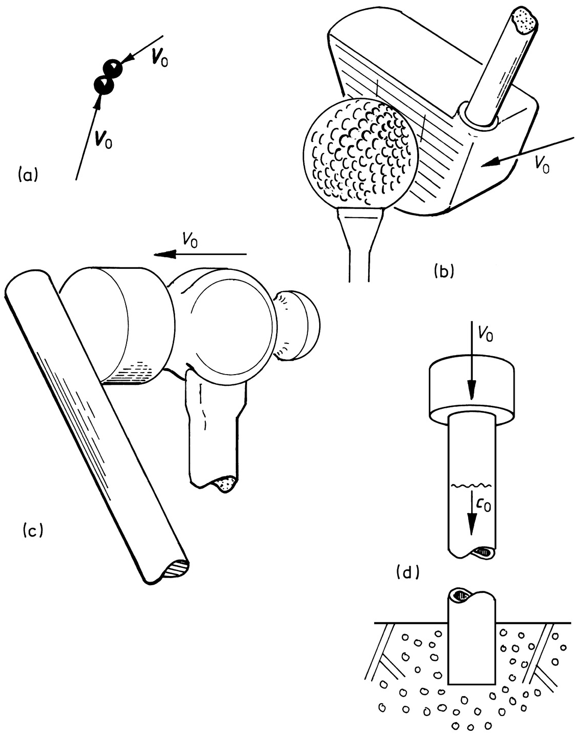
When a bat strikes a ball, or a hammer hits a nail, the surfaces of two bodies come together with some relative velocity at an initial instant termed incidence. After incidence, there would be interference or interpenetration of the bodies were it not for the interface pressure that arises in a small area of contact around the initial contact point between the two bodies. At each instant during the contact period, the pressure in the contact area results in local deformation and consequent indentation; this indentation just equals the interference that would exist if the bodies were not deformed.
At each instant during impact the interface or contact pressure has a resultant force of action or reaction that act in opposite directions on the two colliding bodies and thereby resist interpenetration. Initially, the force increases with increasing indentation and it slows the speed that the bodies are approaching each other. At some instant during impact the work done by the contact force is sufficient to bring the speed of approach of the two bodies to zero. There is a transition at this time from compression to restitution; i.e., from a normal relative velocity of approach to one of separation. During restitution, the energy stored during compression drives the two bodies apart until finally they separate with some relative velocity. For impact between solid bodies, the contact force that acts during collision is consistent with the local deformations that are required for the surfaces of the two bodies to conform in the contact area.
The local deformations that arise during impact vary according to the incident or relative velocity at the point of initial contact and the hardness of the colliding bodies. Slow speed collisions result in contact pressures that cause small deformations only; these are significant solely in a small region adjacent to the contact area. At higher speeds, there are large deformations (i.e., strains) near the contact area that result from plastic flow; these large localized deformations are easily recognizable since they have gross manifestations such as cratering or penetration. In each case, the deformations are consistent with the contact force that causes velocity changes in the colliding bodies. The normal impact speed required to cause large plastic deformation is between 102 × VY and 103 × VY, where VY is the minimum relative speed required to initiate plastic yield in the softer body (for metals the normal incident speed at yield VY is of the order of 0.1 m s−1). This text explains how dynamics of slow-speed collisions are related to both local and global deformations in the colliding bodies.
1.1 Terminology of Two-Body Impact
1.1.1 Configuration of Colliding Bodies
As two colliding bodies approach each other, there is an instant of time, termed incidence, when a single contact point C on the surface of the first body B initially comes into contact with point C′ on the surface of the second body B′. This time t = 0 is the initial instant of impact. Ordinarily the surface of at least one of the bodies has a continuous gradient at either C or C′ (i.e., at least one body has a topologically smooth surface) so that there is a unique common tangent plane that passes through the coincident contact points C and C′. The orientation of this plane is defined by the direction of the normal vector n; a unit vector which is perpendicular to the common tangent plane.
Central or Collinear Impact Configuration
If each colliding body has a center of mass G or G′ that is on the common normal line passing through C, the impact configuration is collinear or central. This requires that the position vector rC from G to C, and the vector  from G′ to C, are both parallel to the common normal line as shown in Figure 1.1a,
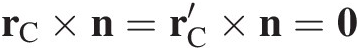
Collinear impact configurations result in equations of motion for normal and tangential directions that can be decoupled. If the configuration is not collinear, the configuration is eccentric.
Figure 1.1 Colliding bodies B and B′ with (a) collinear and (b) non-collinear impact configurations. In both cases the angle of incidence is oblique; i.e., ψ0≠0.
Eccentric Impact Configuration
The impact configuration is eccentric if at least one body has a center of mass that is off the line of the common normal passing through C as shown in Figure 1.1b. This occurs if either

If the configuration is eccentric and the bodies are rough (i.e., there is a tangential force of friction that opposes sliding), the equations of motion involve both normal and tangential forces (and impulses). Thus, eccentric impact between rough bodies involves effects of friction and normal forces that are not separable.
1.1.2 Relative Velocity at Contact Point
At the instant when colliding bodies first interact, the coincident contact points C and C′ have an initial or incident relative velocity  . The initial relative velocity at C has a component normal to the tangent plane v0 ⋅ n and a component tangential to the tangent plane (n × v0) × n; the latter component is termed sliding. The angle of incidence ψ0 is the angle between the initial relative velocity vector v0 and the normal to the common tangent plane n, i.e.,

The angle of incidence can be either positive or negative; it takes the same sign as the initial direction of tangential relative velocity.
Direct impact occurs when in each body the velocity field is uniform and parallel to the normal direction. Direct impact requires that the angle of obliquity at incidence equals zero, ψ0 = 0; on the other hand, oblique impact occurs when the angle of incidence is nonzero, ψ0≠0.
1.1.3 Interaction Force
An interaction force and the impulse that it generates can be resolved into components normal and tangential to the common tangent plane. For particle impact the impulse is considered to be normal to the contact surface and due to short-range interatomic repulsion. For solid bodies however, contact forces arise from local deformation of the colliding bodies; these forces and their associated deformations ensure compatibility of displacements in the contact area and thereby prevent interpenetration or overlap of the bodies. In addition, a tangential force, friction, can arise if the bodies are rough and there is sliding in the contact area. Dry friction is negligible if the bodies are smooth.
Conservative forces are functions solely of the relative displacement of the interacting bodies. In an elastic collision, the forces associated with attraction or repulsion are conservative (i.e., reversible); it is not necessary, however, for friction (a nonconservative force) to be negligible. In an inelastic collision the interaction forces (other than friction) are nonconservative, so that there is a loss of kinetic energy as a result of the cycle of compression and restitution that gives rise to the interaction force acting in the contact region. The energy loss can be due to irreversible elastic-plastic material behavior, rate-dependent material behavior, elastic waves trapped in the separating bodies, etc.
1.2 Classification of Methods for Analyzing Impact
To classify collisions into specific types which require distinct methods of analysis, we need to think about the deformations that develop during collision, the distribution of these deformations in each of the colliding bodies, and how these deformations affect the period of contact. In general, there are four types of analysis for slow-speed collisions and they are associated with particle impact, rigid-body impact, transverse impact on flexible bodies (i.e., transverse wave propagation or vibrations), and axial impact on flexible bodies (i.e., longitudinal wave propagation). A typical example where each method applies is illustrated in Figure 1.2.
(a) Particle impact is an analytical approximation that considers a normal component of interaction impulse only. By definition, particles are smooth and spherical. The source of the interaction force is unspecified but presumably it is strong and very short range so that the period of interaction is a negligibly small instant of time.
(b) Rigid-body impact occurs between compact bodies where the contact area remains small in comparison with all section dimensions. Stresses generated in the contact area decrease rapidly with radial distance from the contact region, so the internal energy of deformation is concentrated in a small region surrounding the interface. This small deforming region has large stiffness and acts much like a short but very stiff spring separating the colliding bodies at the contact point. The period of contact depends on the normal compliance of the contact region and an effective mass of the colliding bodies.
(c) Transverse impact on flexible bodies occurs when at least one of the bodies suffers bending as a result of the interface pressures in the contact area; bending is significant at points far from the contact area if the depth of the body in the direction normal to the common tangent plane is small in comparison with dimensions parallel to this plane. This bending reduces the interface pressure and prolongs the period of contact. Bending is a source of energy dissipation during collision in addition to the energy loss due to local deformation that arises from the vicinity of contact. This can occur in beams, plates, or shells.
(d) Axial impact on flexible bodies generates longitudinal waves which affect the dynamic analysis of the bodies only if there is a boundary equidistant from the impact point which reflects the radiating wave back to the impact point; it reflects the outgoing wave as a coherent stress pulse that travels back to its source essentially undiminished in amplitude. In this case the time of contact depends on the transit time for a wave traveling between the impact surface and the distal surface. Ordinarily this time will be less than that for rigid body impact between hard bodies with convex surfaces.

Figure 1.2 Impact problems requiring different analytical approaches: (a) particle impact, (b) rigid-body impact, (c) transverse deformations of flexible bodies, and (d) axial deformation of flexible bodies.
1.2.1 Description of “Rigid Body” Impact
For bodies that are hard (i.e., with small compliance) only very small deformations are required to generate very large contact pressures; if the surfaces are initially nonconforming, the small deformations imply that the contact area remains small throughout the contact period. The interface pressure in this small contact area causes the initially nonconforming contact surfaces to deform until they conform or touch at most if not all points in a small contact area. Although the contact area remains small in comparison with cross-sectional dimensions of either body, the contact pressure is large and it gives a large stress-resultant or contact force. The contact force is large enough to rapidly change the normal component of relative velocity across the small deforming region that surrounds the contact patch. The large contact force rapidly accelerates the bodies and thereby limits interference which would otherwise develop after incidence if the bodies did not deform.
Hence in a small region surrounding the contact area the colliding bodies are subjected to large stresses and corresponding strains that can exceed the yield strain of the material. At quite modest impact velocities (on the order of 0.1 m s−1 for impact between bodies composed of structural metals) irreversible plastic deformation begins to dissipate some energy during the collision; consequently, there is some loss of kinetic energy of relative motion in all but the most benign collisions. Despite large stresses in the contact region, the stresses decay rapidly with increasing distance from the contact surface. In an elastic body with a spherical coordinate system centered at the initial contact point, the radial component of stress σr decreases very rapidly with increasing radial distance r from the contact region (in an elastic solid σr decreases as r−2 in a 3D deformation field). For a hard body the corresponding rapid decrease in strain means that significant deformations occur only in a small region around the point of initial contact; consequently, the deflection or indentation of the contact area remains very small.
Since the region of significant strain is not very deep or extensive, hard bodies have very small compliance (i.e., a large force generates only a small deflection). The small region of significant deformation is like a short stiff spring, which is compressed between the two bodies during the period of contact. This stiff spring with a large spring constant gives a very brief period of contact. For example, a hard-thrown baseball or cricket ball striking a bat is in contact for a period of roughly two milliseconds (2 ms) while a steel hammer striking a nail is in contact for a period of about 0.2 ms. The contact duration for the hammer and nail is smaller because these colliding bodies are composed of harder materials than the ball and bat. Both collisions generate a maximum force on the order of 10 kN (i.e., roughly one ton).
From an analytical point of view, the most important consequence of small compliance of hard bodies is that very little movement occurs during the very brief period of contact; i.e., despite large contact forces there is insufficient time for the bodies to displace significantly during impact. This observation forms a fundamental hypothesis of rigid body impact theory; namely that for hard bodies, analyses of impact can consider the period of contact to be vanishingly small so that changes in velocity occur instantaneously (i.e., in the initial or incident configuration). The system configuration at incidence is termed the impact configuration. This theory assumes there is no movement during the contact period.
Underlying Premise of Rigid Body Impact Theory
a. In each of the colliding bodies the contact area remains small in comparison with both the cross-sectional dimensions and the depth of the body in the normal direction.
b. The contact period is sufficiently brief that during contact the displacements are negligible and hence there are no changes in the system configuration; i.e., the contact period can be considered to be instantaneous.
If these conditions are approximately satisfied, rigid body impact theory can be applicable. In general, this requires that the bodies be hard and that they suffer only small local deformation in collision. For a solid composed of material that is rate-independent, a small contact area results in significant strains only in a small region around the initial contact point. If the body is hard the very limited region of significant deformations causes compliance to be small and consequently, the contact period to be very brief. This results in two major simplifications.
a. Equations of planar motion are trivially integrable to obtain algebraic relations between velocity changes and the reaction impulse.Footnote 1
b. Finite active forces (e.g. gravitational or magnetic attraction) which act during the period of contact can be considered to be negligible since these forces do no work during the collision.
During the contact period the only significant active forces are reactions at points of contact with other bodies; these reactions are induced by displacement constraints.
Figure 1.3 shows a collision where application of rigid body impact theory is appropriate. This series of high speed photographs shows development of a small area of contact when an initially stationary field hockey ball is struck by a hockey stick at an incident speed of 18 ms−1. During collision the contact area increases to a maximum radius aC that remains small in comparison with the ball radius R′; in Figure 1.3, aC/R′ < 0.2. This small contact area is a consequence of the small normal compliance (or large elastic modulus) of both colliding bodies and the initial lack of conformation of the surfaces around the initial contact point.

A useful means of postulating rigid body impact theory is to suppose that two colliding bodies are separated by an infinitesimal deformable particle.Footnote 2 The deformable particle is located between the point of initial contact on one body and that on the other, although these points are coincident. The physical construct of an infinitesimal compliant element separating two bodies at a point of contact allows variations in velocity during impact to be resolved as a function of the normal component of impulse. This normal component of impulse is equivalent to the integral of the normal contact force over the period of time after incidence. Since collisions between bodies with nonadhesive contact surfaces involve only compression of the deformable particle – never extension – the normal component of impulse is a monotonously increasing function of time after incidence. Thus, variations in velocity during an instantaneous collision are resolved by choosing as an independent variable the normal component of impulse rather than time. This gives velocity changes which are a continuous or smooth function of impulse.
There are three notable classes of impact problems where rigid body impact theory is not applicable if the impact parameters representing energy dissipation are to have any range of applicability. (a) The first involve impulsive couples applied at the contact point. Since the contact area between rigid bodies is negligibly small, impulsive couples are inconsistent with rigid body impact theory. To relate a couple acting during impulse to physical processes, one must consider the distribution of deformation in the contact region. Then the couple, due to a distribution of tangential force, can be obtained from the law of friction and the first moment of tractions in a finite contact area about the common normal through the contact point. (b) A second class of problems where rigid body impact theory does not apply is axial impact of collinear rods with plane ends. These are problems of one dimensional wave propagation where the contact area and cross-sectional area are equal because the contacting surfaces are conforming; in this case the contact area may not be small. In these problems, deformations and particle velocities far from the contact region are not insignificant. As a consequence, for one-dimensional waves in long bars, the contact period is dependent on material properties and depth of the bars in a direction normal to the contact plane rather than compliance of local deformation near a point of initial contact. (c) The third class of problems where rigid body theory is insufficient are transverse impacts on beams or plates where vibration energy is significant.
Collisions with Compliant Contact Points of Otherwise “Rigid” Bodies
While most of our attention will be directed toward rigid body impact, there are cases where distribution of stress is significant in the region surrounding the contact area. These problems require consideration of details of local deformation of the colliding bodies near the point of initial contact; they are analyzed in Chapters 6 and 8. The most important example may be collisions in multi-bodied systems where the contact points do not have substantial increase in compliance as the contact becomes more remote from any point of external impact; i.e., a compliant contact theory is required if all contacts have similar stiffness or compliance. Considerations of local compliance may be represented by discrete elements such as springs and dashpots or they can be obtained from continuum theory. Also, for collisions between bodies where an irreversible compliance can be obtained for each body, this compliance can be used to calculate energy loss during collision and thereby evaluate the coefficient of restitution as a function of incident velocity at the impact point. To obtain the local distribution of strain (and stress) near the contact region of deformable bodies from continuum theory, the artifice of a deformable particle separating the contact points needs to be abandoned. Instead we seek a distribution of contact pressure which results in compatible surface displacements inside the periphery of the contact area; i.e., the pressure distribution must be determined which causes the surfaces of initially nonconforming bodies to touch at each point inside a contact radius without interpenetration.
1.2.2 Description of Transverse Impact on Flexible Bodies
Transverse impact on plates, shells, or slender bars results in significant flexural deformations of the colliding members both during and following the contact period. In these cases, the stiffness of the contact region depends on flexural rigidity of the bodies in addition to continuum properties of the region immediately adjacent to the contact area; i.e., it is no longer sufficient to suppose that a small deforming region is surrounded by a rigid body. Rather, flexural rigidity is usually the more important factor for contact stiffness when impact occurs on a surface of a plate or shell structural component.
1.2.3 Description of Axial Impact on Flexible Bodies
Elastic or elastic-plastic waves radiating from the impact site are present in every impact between deformable bodies – in a deformable body, it is these radiating waves that transmit variations in velocity and stress from the contact region to the remainder of the body. Waves are an important consideration for obtaining a description of the dynamic response of the bodies, however, only if the period of collision is determined by wave effects. This is the case for axial impact acting uniformly over one end of a slender bar if the far or distal end of the bar terminates in a reflective boundary condition. Similarly, for radial impact at the tip of a cone, elastic waves are important if the cone is truncated by a spherical surface with a center of curvature at the apex. In these cases where the impact point is also a focal point for some reflective distal surface, the wave radiating from the impact point is reflected from the distal surface and then travels back to the source where it affects the contact pressure. On the other hand, if different parts of the outgoing stress wave encounter boundaries at various times and these surfaces are not normal to the direction of propagation, the wave will be reflected in directions that are not towards the impact point; while the outgoing wave changes the momentum of the body, this wave is diffused rather than returning to the source as a coherent wave that can change the contact pressure and thereby affect the contact duration.
1.2.4 Applicability of Theories for Low-Speed Impact
This text presents several different methods for analyzing changes in velocity (and contact forces) resulting from low-speed impact; i.e., where the bodies are not significantly deformed by impact. These theories are listed in Table 1.1 with descriptions of the differences and an indication of the range of applicability for each.
Table 1.1 Applicability of theories for oblique, low-speed impact
| Impact theory | Indep. variable | Coeff.restitution | Angle of incidence at impact pt.ψ0 | Spatial grad. of contact complianceα | (Impact pt. compliance) / (structural compliance) | Computational effort | Illustration |
|---|---|---|---|---|---|---|---|
| Stereo-mechanical (non-smooth dyn.) | none | e, e0, e∗ | >tan−1(μβ1/β3) | > 1 | >> 1 | low |  |
| Rigid body (smooth dynamics) | normal | >tan−1(μβ1/β3) | |||||
| impulse | |||||||
| p | e∗ | > 1 (sequential) | >> 1 | low |  | ||
| << 1 (simultaneous) | |||||||
| Compliant contact (smooth dynamics) | time | ||||||
| t | e∗ | all | all | >> 1 | moderate |  | |
| Continuum (smooth dynamics) | time | ||||||
| t | none | all | all | all | high |  |
e, e0, e∗= kinematic, kinetic, energetic coefficients of restitution
μ = Amontons–Coulomb coefficient of limiting friction;
β1, β3= inertia coefficients (see Chap 3).
The stereo-mechanical theory is a relationship between incident and final conditions; it results in discontinuous changes in velocity at impact. In this book a more sophisticated rigid body theory is developed – a theory in which the changes in velocity are a continuous function of the normal component of the impulse p at the contact point. This theory results from considering that the coincident points of contact on two colliding bodies are separated by an infinitesimal deformable particle – a particle that represents local deformation around the small area of contact. With this artifice, the analysis can follow the process of slip and/or slip-stick between coincident contact points if the contact region has negligible tangential compliance. Rigid body theories are useful for analyzing two-body impact between compact bodies composed of stiff materials; however, they have limited applicability for multi-body impact problems.
When applied to multi-body problems, rigid body theories can give accurate results only if the set of contacts that connect rigid bodies has a local contact compliance that is either decreasing or increasing with distance from the point of external impact. If the contact compliances that connect a set of rigid bodies are decreasing with increasing distance from the point of external impact, then the separate reactions essentially occur simultaneously. On the other hand, if the set of contacts have increasing local contact compliance with increasing distance from the point of external impact, then the reactions occur sequentially, with a delay that increases with distance from the point of external impact. This second case is essentially one of wave propagation. Generally, the reaction forces at points of contact arise from infinitesimal relative displacements that develop during impact; these reaction forces are coupled when they overlap.
If, however, other points of contact or cross-sections of the body have compliance of the same order of magnitude as that at any point of external impact, then the effect of these flexibilities must be incorporated into the dynamic model of the system. If the compliant elements are local to joints or other small regions of the system, an analytical model with local compliance may be satisfactory (e.g., see Chapter 8). On the other hand, if the body is slender so that significant structural deformations develop during impact, either a wave propagation or a structural vibration type analysis may be required (see Chapters 7 and 10). Whether the distributed compliance is local to joints or continuously distributed throughout a flexible structure, these theories require a time-dependent analysis to obtain reaction forces that develop during contact and affect the changes in velocity in the system.
Hence, the selection of an appropriate theory depends on structural details and the degree of refinement required to obtain the desired information.
1.3 Principles of Dynamics
1.3.1 Particle Kinetics
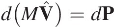
The fundamental form of most principles of dynamics is in terms of dynamics of a particle. A particle is a body of negligible or infinitesimal size; i.e., a point mass. The particle is the building block that will be used to develop the dynamics of impact for either rigid or deformable solids. A particle of mass M moving with velocity V has momentum MV. If a resultant force F acts on the particle, this causes a change in momentum in accord with Newton’s 2nd law of motion.
Law II: The momentum MV of a particle has a rate-of-change with respect to time that is proportional to and in the direction of any resultant force F(t) acting on the particle.Footnote 3
Usually the particle mass is constant so that Eq. (1.1) can be integrated to obtain the changes in velocity as a continuous function of the impulse P(t).
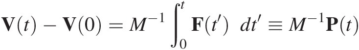 (1.2)
(1.2)This vector expression is illustrated in Figure 1.4.

The interaction of two particles B and B′ that collide at time t = 0 generates active forces F(t) and F′(t) that act on each particle respectively, during the period of interaction, 0 < t < tf; these forces of interaction act to prevent interpenetration. The particular nature of interaction forces depends on their source, i.e., whether they are due to contact forces between solid bodies that cannot interpenetrate or are interatomic forces acting between atomic particles. In any case, the force on each particle acts solely in the radial direction. These interaction forces are related by Newton’s third law of motion.
Laws II and III are the basis for impulse-momentum methods of analysing impact. Let particle B have mass M, and particle B′ have mass M′. Integration of Eq. (1.3) gives equal but opposite impulses −P′(t) = P(t) so that equations of motion for the relative velocity v ≡ V − V′ can be obtained as
where m is the effective mass. The change of variables from velocity V(t) in an inertial reference frame to relative velocity v(t) is illustrated in Figure 1.5. The limit of Eq. (1.4) as the period of contact approaches zero, tf→0, gives the basis of smooth dynamics of collision for particles and rigid bodies.

Figure 1.5 (a) Equal but opposite normal impulses P on pair of colliding bodies with masses M and M′ result in velocity changes P and −M′−1P respectively. (b) Thin lines are initial and final velocity for each body while the thick lines are initial relative velocity v(0), the final relative velocity v(P) and the change in relative velocity m−1P.
A golf ball has mass M = 46 g. When hit by a heavy club the ball acquires a speed of 44.6 ms–1 (100 mph) during a contact duration tf = 0.4 ms (milliseconds). Assume that the force-deflection relation is linear and calculate an estimate of the maximum force Fmax acting on the ball.
Solution
- effective mass
m = 0.046 kg
- initial relative velocity
v(0) = –v0 = –44.6 ms–1
(i) linear spring ⇒ simple harmonic motion for relative displacement δ at frequency ω where
 .
.(ii) change in momentum of relative motion = impulse, Eq. (1.4)
⇒ Fmax = 8.06 kN ( ≈ 0.8 tons)


1.3.2 Kinetics for Set of Particles
For a set of n particles where the ith particle has mass Mi and velocity Vi the equations of translational motion can be expressed as

where Fi is an external force acting on particle i and  is an internal interaction force of particle k on particle i. Since the internal forces are equal but opposite
  , the sum of these forces over all particles vanishes; hence
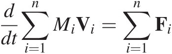 (1.5)
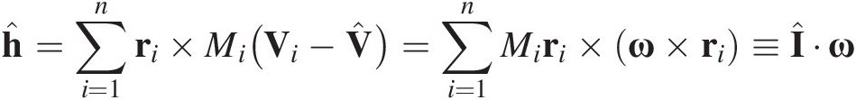
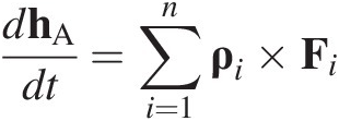
(1.5)The moment of momentum hO of particle i about point O is defined as hO ≡ ρi × MiVi where ρi is the position vector of the particle from O and Mi is the mass of the particle. Thus, the set of particles has a moment of momentum about O,

For a set of n particles the rate of change of moment of momentum about O is related to the moment about O of the external forces acting on the system,
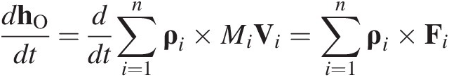 (1.6)
(1.6)If the configuration of the system does not change during the period of time t, integration of (1.6) with respect to time gives
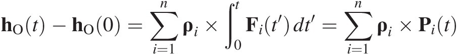 (1.7)
(1.7)1.3.3 Kinetic Equations for Rigid Body
A rigid body can be represented as a set of particles located at positions a fixed distance apart. When the body is moving the only relative velocity between different points on the body is due to angular velocity of the body ω and the distance between the points.
Suppose a body of mass M is composed of particles with mass Mi, i = 1, ⋯, n where the position vector of each particle is ρi in an inertial reference frame with origin at O. The center of mass of this set of particles is located at position  where
where

as illustrated in Figure 1.6. The center of mass has velocity  . Hence for the set of particles that comprise this body, the translational equation of motion Eq. (1.5) can be expressed as
 (1.8)
(1.8)
Translational Momentum and Moment of Momentum
The moment of momentum about O for the body can be expressed in terms of the moment of the translational momentum of the body  plus the couple from the rotational momentum of the body. First note that the position of a particle ρi can be decomposed into the position vector of the center of mass
  plus the position vector of the ith particle relative to the center of mass ri; i.e.,
  . Thus, the moment of momentum about O becomes
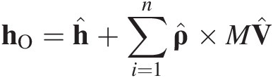
where  is the moment of momentum for the system about the center of mass G,
and  is the inertia dyadic for the center of mass G.Footnote 4
Thus, the equation of motion (1.6) can be expressed as
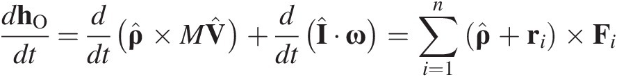 (1.9)
(1.9)This decomposition of the particle position vector  has separated the equation for rate of change of moment of momentum about O into a term for the moment of translational momentum of the body acting at the center of mass and a second term for the moment of momentum relative to the center of mass G.
Noting that the differential of an applied impulse dPi = Fidt we obtain from (1.8) and (1.9) that for a rigid body there are three independent equations of motion in terms of the applied impulse  .
.
 (1.10a)
 (1.10b)
 (1.10c)
Equation (1.10b) is the differential of the moment abut O of translational momentum of the body.
Kinetic Energy
For some problems it is preferable to use a scalar measure of activity of a body; e.g. the kinetic energy T rather than the vectorial representation (1.10). Consider a body composed of n particles so that the kinetic energy T is expressed as
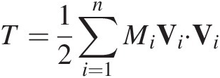
A rigid body has kinetic energy T that can be resolved into translational kinetic energy Tv and rotational kinetic energy Tω,
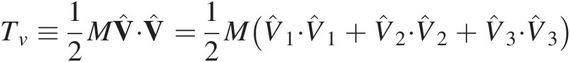 (1.11a)
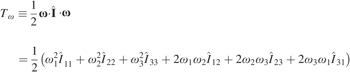 (1.11b)
where  is the velocity of the center of mass, ω is the angular velocity of the body and
  is the inertia dyadic for the center of mass.
Taking the scalar product of (1.10a) with  and (1.10c) with ω we obtain the equation of motion,
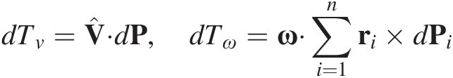 (1.12)
These equations of motion have a right-hand side that is the differential of the rate-of-work of applied impulses and the differential of the rate-of-work of applied torques about the center of mass, respectively. Expressions (1.12) are scalar equations for the change of state of a rigid body subject to a number n of active impulses Pi
A cube is resting on a flat level plane; it has mass M and sides of length 2a. The sides are slightly convex so only the edges touch the plane. One edge of the cube is raised slightly and then released so that when the opposite edge C strikes the surface, the cube is rotating with angular velocity ω−. The impact is perfectly plastic so there is no bounce of edge C. Find the angular velocity ω+ immediately after impact at C and calculate the part of the initial kinetic energy T− that is lost at impact, (T– – T+)/T–.
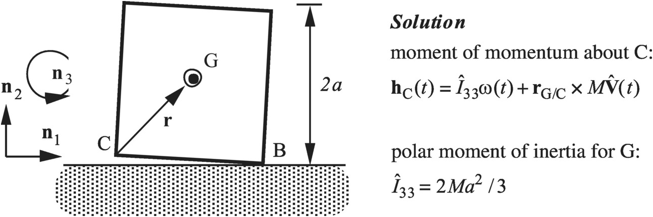
velocity of center of mass:

moment of momentum about impact point C:
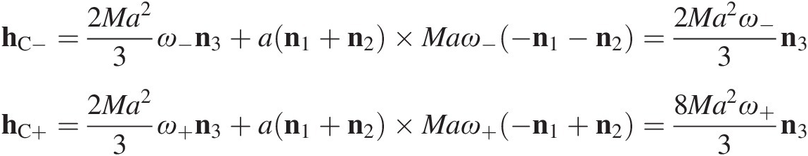
no moment of impulsive forces about impact point C during impact (Eq 1.6):
kinetic energy (planar motion):

part of initial kinetic energy absorbed in impact:
Equation 1.6 relates the moment of forces about the origin to the rate of change of moment of momentum about the origin. Is there a similar relation for moment of forces about a point that is moving?
1.3.4 Rate of Change for Moment of Momentum of System about Point Moving Steadily Relative to Inertial Reference Frame
Let point A be coincident with point O but moving steadily at velocity VA relative to an inertial reference frame and denote the position vector of the ith particle relative to A by ρi. If hA denotes the moment of momentum of the system of n particles with respect to A, then Eq. (1.6) gives the following theorem.
For a system of particles, the rate of change of moment of momentum with respect to point A is equal to the moment of external forces about A if and only if
(i) VA = 0 so that point A is fixed in an inertial reference frame; or
(ii) VA and
are parallel.

In either case,
 (1.13)
During a period t in which the configuration of the system does not vary, Eq(1.13) can be integrated with respect to time to give
 (1.14)
Example 1.3 A system consists of two particles A and B that are connected by a light inextensible string. Particle A with mass 2M is located at rA = (1, 1, 0) and has velocity VA = (1, 0, 0) in a Cartesian reference frame while particle B with mass M is located at rB = (3, 2, 0) and has velocity  . Find (i) the component of velocity
  and the angular velocity ω of the string and (ii) the moment of momentum of the system about the origin 0.
 Solution
- relative position of B from A,
ρB/A ≡ ρB − ρA = (2, 1, 0)
- relative velocity of B from A,
- inextensible string requires,


1.4 Decomposition of a Vector
Any vector v can be decomposed into a component vnn in direction n and a component vte in a direction perpendicular to n.
where

This relation is particularly helpful for analyzing oblique impact of rigid bodies; it is used to resolve the relative velocity and impulse at the contact point into components normal and tangential to the surfaces of colliding bodies.
It is worth noting that the vector v has a component perpendicular to n that can be expressed as alternatively,
1.5 Vectorial and Indicial Notation
Frequently, there is a need to express a vector variable such as velocity V of a point in terms of the components of velocity in some reference frame. Let ni be a set of mutually perpendicular unit vectors fixed in reference frame ℜ. The components of velocity in this reference frame have magnitudes that can be expressed as Vi ≡ V ⋅ ni, i = 1, 2, 3. In vectorial notation the vector is expressed in terms of its components  where the last equality follows from repeated subscripts implying summation over the range of spatial coordinates. On the other hand, in indicial or shorthand notation V ≡ Vi (i.e., unit vectors) are implied rather than written explicitly. Similarly, if r denotes the position of C relative to a point O fixed in ℜ, then in vectorial notation r ≡ ri ni or in indicial notation r ≡ ri.
As a consequence of these definitions, the inner or dot product can be expressed in alternative forms,
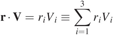 (1.16)
where a repeated subscript (e.g. i) implies summation over the range of spatial coordinates. Likewise, the vector or cross product can be expressed as,
 (1.17)
where εijk is the permutation tensor which has values εijk = + 1 if indices are in cyclic order, εijk = –1 if indices are in anticyclic order and εijk = 0 if an index is repeated.
Problems
1.1 An initially stationary wood block of mass M is struck at the center of one side by a bullet of mass M′ that strikes at a normal incident speed V0. The bullet is captured by the block. Find the final speed of the block and calculate an estimate the fraction of the bullet’s initial kinetic energy T0 that is transformed to heat.
1.2 Direct impact of a body with mass M(g) against a rigid wall at an incident velocity V0(ms–1) results in a contact duration tf (ms). For a collision conditions (M, V0, tf.), calculate an estimate of the maximum force Fmax(N) during a collision of each of the following bodies: tennis ball (45, 44, 4.0); golf ball (46, 44, 0.6); ping-pong ball (2.5, 44, 0.5), steel hammer (103, 1, 0.2).


1.4 A rigid uniform bar of mass M and length 3L lies across two parallel rails B and B′ that are separated by width L. The bar is transverse to the rails and centered. The end closest to B′ is raised a small distance and then released so that the bar is rotating with angular speed ω– when it strikes B′.
a. Find the ratio of angular speeds of the bar ω+/ω– at the instant immediately after impact if the impact with rail B′ is perfectly plastic.
b. Find the ratio of angular speeds of the bar ω+/ω– at the instant immediately after impact if the impact with rail B′ is elastic.
c. Obtain the fraction of the incident kinetic energy T– that finally is lost as a result of collision (a).
1.5 A prismatic cylinder with polygonal cross-section has n equal sides where n ≥ 4. Between adjacent sides a regular polygon has an included angle 2α where α = π/n. Let the prismatic cylinder of mass M have a radius a from the center O to each vertex Ci. Find that this prismatic cylinder has a polar moment of inertia  for the center of mass O where
  .
.
If the cylinder is rolling on a flat and level surface and before vertex Ci impacts with the surface it has angular speed ω(–). Obtain an expression for the angular speed ω(+) the instant after vertex Ci strikes the surface. Assume that after impact, vertex Ci remains in contact with the surface.
1.6 A wheel of radius a and radius of gyration for the center of mass  rolls upon a rough horizontal surface which may be idealised as a series of uniform saw-toothed serrations of pitch 2b. The wheel rolls without slip or elastic rebound on the tips of the serrations under the action of a constant horizontal force F applied at its center.
(a) Show that at each impact the ratio of angular speed at separation to that at incidence satisfies
(b) Find that when steady conditions are reached the wheel moves with a fluctuating forward velocity and
where v1 is the maximum forward component of velocity in each cycle.


1.7 For vectors r = {r1, r2, r3 }T and V = {V1, V2, V3 }T verify that r × V = εijkrjVk.