


Introduction
Nuclear magnetic resonance (NMR) imaging has been successfully applied to medical imaging over the last several years (Reference Partain, Price, Patton, Kulkarni and JamesPartain and others, 1988). NMR is particularly sensitive to the proton magnetic moment which occurs in water and organic compounds. The proton is the nearly 100% abundant isotope of hydrogen and has the largest magnetic moment of any nucleus except tritium. This is helpful since the signal-to-noisc ratio (SNR) is proportional to μ5/2 (Reference AndrewAndrew, 1969), where μ is the magnetic moment, and SNR determines the limits of spatial resolution.
NMR is done by placing the sample of interest in a strong, uniform magnetic field. Radiofrequency (RF) coils are used to apply an RF magnetic field to the sample and to receive signals back from precessing nuclei in the sample (Reference AndrewAndrew, 1969).
Imaging additionally requires the use of gradient magnetic field windings, which apply linearly varying fields in the x-, y- and z-directions. The application of gradients causes nuclei at different positions in the sample to precess at different frequencies. The strength of the signal at a particular frequency is proportional to the fluid density at the corresponding spatial position. So the spatial distribution of the magnetization density in the sample is encoded as a position-dependent phase and frequency distribution of magnetization which enables formation of the image.
NMR relaxation times, which are the time for the magnetization to decay to its equilibrium value, play an esssential role in producing contrast in images (Reference Partain, Price, Patton, Kulkarni and JamesPartain and others, 1988). For example, liquids have long relaxation times (a few seconds for water) while in solids the transverse magnetization, which is detected by a radiofrequency (RF) coil, may decay in μs. Thus, in saltwater ice, it is evident that there should be substantial contrast between the liquid water which exists to about −22°C (i.e. the eutectic temperature in the H2O-NaCl system) and the surrounding ice (Reference Mikhaylov and ChizhikMelnichenko and others, 1979; Reference Ocampo and KlingerOcampo and Klinger, 1983).
Materials And Methods
Columnar ice was prepared (Reference Kuehn, Lee, Schulson, Sodhi, Luk and SinhaKuehn and others, 1988) from a solution consisting of Hanover town water with 20 ppt of sea saltsFootnote * in a 10001 tank, 3 ft [0.91m] in diameter. The grain-size is about 4 mm diameter with length 5–17 mm. The salinity of the ice melt water was 4.3 ppt and was determined using a temperature-compensated conductivity meter. The solution was equilibrated at 0°C and then cooled from the top by an aluminum plate maintained at −20°C in contact with the top of the solution. Unidirectional freezing took place over a period of 14 d at which point the ice was about 300 mm thick. Subsequently, the block was removed from the tank and 100 mm diameter test specimens were cored in the direction of freezing. The specimen diameters were then reduced to 50 mm by machining in a lathe.

Fig. 1. Apparatus for NMR imaging of ice samples. 50 mm diameter salt-water ice samples were placed in an acrylic plastic chamber 55 mm i.d. × 230 mm long and cold nitrogen gas obtained from a liquid-nitrogen dewar was passed over the sample. The gas temperature was controlled by a heater around a sintered copper plug and a temperature controller which monitored the ice temperature with a thermocouple.
In further experiments, about 1 ppt of Cu2SO4 was added to the solution in order to shorten the NMR relaxation time of the water and thereby enable faster data acquisition. Note that the Cu2SO4 concentration was much lower than the sea-salt concentration and thus the presence of the Cu2SO4 should not significantly affect the ice freezing point.
The NMR imaging system (Reference Edelstein, Vinegar, Tutunjian, Roemer and MuellerEdelstein and others, 1988) is a 2 Tesla, 310 mm bore magnet operating at a proton NMR frequency of 85 MHz. The field gradients used in this study have an inner diameter of about 150 mm and a maximum strength of about 180 mTm−1. Because they are shielded, the gradient-rise times are short which enables early data acquisition (Reference Edelstein, Vinegar, Tutunjian, Roemer and MuellerEdelstein and others, 1988).
A small temperature-controlled chamber with dimensions about 55 mm i.d. by 230 mm long was constructed from acrylic plastic. The chamber was fed by cold nitrogen gas passing through a sintered copper plug wrapped by heating tape (Thermolyne Co.). The temperature in the chamber was sensed by a thermocouple which was plugged into a controller (Research Inc., model 61011) which fed back through a solid-state relay and controlled the temperature (Fig. 1). The temperature of the ice was sensed by a thermocouple inserted into one end of the core. A second thermocouple was inserted into the opposite end of the core for one experiment, and, after equilibration, the temperature difference between the ends of the core was measured to be less than 2°C.
The imaging was done with a 256 × 256 matrix (1/2 mm × 1/2 mm resolution) with a 5 mm slice thickness. The total imaging time was about 5 m.
Results
Imaging was easily achieved in ice cylinders at temperatures down to −20°C. Since we were using a spin-echo of a few ms, it is likely that the NMR-visible protons were in the form of liquid water. In general, less material was visible as the temperature was lowered, and an image attempted at −24°C showed essentially no signal. Figure 2a shows a cross-sectional image of a 2 in cyclinder, made without Cu2SO4, at −14°C. Brine appears as bright features. Figure 2b shows a longitudinal section image of the same cylinder. There is some distortion apparent which makes the ends of the cylinder seem narrower than the center; this is caused by non-linearity of the gradient magnetic fields over the cylinder length. Note the relative absence of structure in the longitudinal section, showing that there is not much change in the distribution of entrapped brine as a function of position along the cylinder. This pattern is consistent with the columnar grain structure and platelet-like array of brine pockets aligned with the axis of the column.
Figure 3a is a cross-section image of another ice cyclinder, made using 1 ppt Cu2SO4, taken at −11°C. Figure 3b shows the same cylinder at −4°C where the brine pockets/channels are considerably larger. The bright areas observed in Figure 3 are reminiscent of drainage channels seen in horizontal views of thin plates of sea ice from Saroma Lagoon, Hokkaido, Japan, (Reference Wakatsuchi and SaitoWakatsuchi and Saito, 1985). Whether the bright regions shown by NMR are indeed drainage channels, but on a finer scale than those shown by Reference Wakatsuchi and SaitoWakatsuchi and Saito (1985), needs confirmation by further work.
Discussion
NMR imaging has the ability to image structure inside salt-water ice which is difficult to visualize non-destructively within the intact volume by any other means. NMR is particularly good at seeing liquid water inside ice, but it is conceivable that NMR might even look at solid parts of the ice. It is reasonable to envisage NMR imaging being carried out with the ice in an apparatus which subjects it to mechanical stresses, in which case the NMR may be able to visualize some of the details of the deformation.
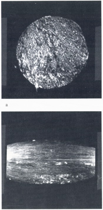
Fig. 2. (a) Cross-sectional image of a 50 mm [2 in] diameter cylinder, made without Cu2SO4, at −14°C. Brine appears as bright features, (b) Longitudinal section of the same cylinder. The shape distortion and extra brightness at the ends of the image are caused by non-linearity of the gradient magnetic field over the cylinder length. Note the relative absence of structure in the longitudinal section, which is consistent with a slow variation of the cross-sectional structure along the length of the cylinder.

Fig. 3. Cross-sectional images of a 50 mm [2in] diameter ice cyclinder containing dissolved Cu2SO4. (a) Cylinder at −11°C; (b) Cylinder at −4°C. Note the enlargement of the brine pockets/channels at the higher temperature.
Acknowledgements
We should like to thank Mr L. Beha of the GE Research and Development Center for his work in assembling and operating the ice-cooling chamber. One of us (E.M.S.) would like to acknowledge support from the U.S. Office of Naval Research under grant N0014–86K-0695.


