


1. Introduction
Turbulent mixing is a ubiquitous problem that arises in many configurations with the aim of mixing fluids through the cascade of three mechanisms, i.e. entrainment, dispersion and diffusion. Depending on the physical and chemical properties of fluids, mixing can be further categorized into ‘passive-scalar mixing’, ‘mixing coupled to dynamics’ and ‘mixing that alters the fluid’ (Dimotakis Reference Dimotakis2005), where the first two categories are the subject of this study. In the simplest case, mixing substances with matched physical properties (e.g. viscosity, density), henceforth constant-viscosity mixing (CVM), is decoupled from the flow dynamics, and thus, only the flow field affects the mixing dynamics, i.e. advection. One way that leads to coupled dynamics is the mixing of fluids with disparate viscosity, henceforth variable-viscosity mixing (VVM), since the variations in viscosity alter, including but not limited to, the local momentum field and Reynolds number. Therefore, the local topology of entrainment and dispersion are perturbed by the observed viscosity gradients while the ratio of momentum diffusivity and mass diffusivity, defined with Schmidt number ( $Sc=\nu / D$), is varied by the magnitude of local viscosity.
In the simulations the range of  $Sc$ has significance from the calculations standpoint such that, in the mixing of liquids ( $Sc\gg 1$), the smallest length scale of the flow field and scalar field eddies are separated by several orders of magnitude. A relation for the smallest length scale defined by Batchelor (Reference Batchelor1959) reads
 \begin{equation} \lambda_B \equiv C_B \lambda_K Sc^{{-}1/2} \equiv C_B \lambda_K \left(\frac{\nu}{D}\right)^{{-}1/2}, \end{equation}
where  $\lambda _B$ is the smallest scalar length scale, $\lambda _K$ is the smallest velocity scale, $C_B$ is a model constant (in the order of unity), $\nu$ is kinematic viscosity, $D$ is the molecular diffusion coefficient and $Sc$ is Schmidt number. It is evident in the correlation that the resulting Schmidt number is a spatiotemporal parameter in VVM and it can be of the order of $\sim 10^5$ in this study. So, in the viscous-convective subrange, the diffusion becomes limited and viscosity prevails (Sreenivasan Reference Sreenivasan2019). The level of segregation between diffusive and viscous scales poses challenges in capturing the mixing physics both experimentally and computationally. Specifically, in the coupled scenario, where viscosity varies by the mixing, the cruciality of accurate modelling is pronounced.
The variation in the viscosity brings fundamentally distinct mixing modes as it dictates the local Reynolds number. The bulk dynamics of the mixing chamber are described by the flow regime of the jet, coflow and completely mixed flows (Mikhail Reference Mikhail1960; Razinsky & Brighton Reference Razinsky and Brighton1971, Reference Razinsky and Brighton1972; Pathikonda et al. Reference Pathikonda, Usta, Ahmad, Khan, Gillis, Dhodapkar, Jain, Ranjan and Aidun2021). In a coaxial jet configuration the acronym describes the flow regime (T for turbulent, L for laminar) of the jet, coflow and fully mixed downstream, respectively. The regimes are determined a priori based on the flow rate, characteristic length and viscosity, i.e. Reynolds number. In this study we focus on TTT ( $m=1$) and TLL ( $m=10$, $20$,
$20$,  $40$) modes. Here, $m$ is defined as the viscosity ratio between the coflow and jet. In the TTT mode, the mixing layer remains turbulent and the typical cascade of the mechanism described earlier applies here. However, in the TLL mode, more complex transport and mixing phenomena are introduced by having a turbulent/non-turbulent interface (TNTI) near the jet entrance and transitioning to laminar flow in downstream locations. One also observes non-zero viscosity gradients that alter the momentum field until all the gradients are diminished by the complete mixing. These ramifications compel us to redefine the key mixing mechanisms.
In this perspective, we identify four distinct mechanisms in the TLL mode to break down all scales of unmixed parcels. These are listed as turbulent mixing, unsteady laminar mixing, steady laminar stretching (under linear velocity gradient in the radial direction) and molecular diffusion sorted in descending order of mixing time scales. Inherently, the first two mechanisms contain positive Q criterion, i.e. areas where the vorticity magnitude is greater than the magnitude of strain rate (Kolář Reference Kolář2007), that promotes engulfment and entrainment of unmixed or poorly mixed fluid parcels. Once the flow transitions to fully developed steady laminar flow, the mixing only occurs through the rather slow processes of shear and molecular diffusion. In particular, in a pipe the shearing varies linearly in the radial direction and it stretches the remaining scalar structures that lead to thin layers of stratified structures, called lamella. This mechanism works in favour of molecular diffusion in a way that it increases interface area while decreasing the characteristic length of diffusion.
If we recall the turbulent mixing mechanism, it requires further elucidation for the TLL mixing mode since the mixing layer has anisotropy in the flow state. When a turbulent jet is issued into a coflowing laminar jet, a highly convoluted TNTI forms at the outermost boundary of the turbulent jet. Starting with the studies of Brown & Roshko (Reference Brown and Roshko1974) and later many other studies (Dahm & Dimotakis Reference Dahm and Dimotakis1987; Ferré et al. Reference Ferré, Mumford, Savill and Giralt1990; Dimotakis Reference Dimotakis2000) concluded on the existence of large-scale organized structures, i.e. advective flux (‘engulfing’ process), that are responsible for the entrainment. However, a fundamental understanding of TNTI with irrotational outer flow carried out by Westerweel et al. (Reference Westerweel, Fukushima, Pedersen and Hunt2005, Reference Westerweel, Fukushima, Pedersen and Hunt2009) indicates a very limited contribution of large-scale motions, instead the entrainment is dominated by small-scale eddying, i.e. viscous stress (‘nibbling’ process), at the high shear interface. Their assertion was also found to be consistent with other studies (Mathew & Basu Reference Mathew and Basu2002; Kohan & Gaskin Reference Kohan and Gaskin2020). Furthermore, the ground-breaking experiments and multiscale analysis by Philip et al. (Reference Philip, Meneveau, de Silva and Marusic2014) showed that while large-eddy simulation (LES)-type modelling reasonably captures the ‘nibbling’ process, Reynolds-averaged Navier–Stokes (RANS)-type models govern the entrainment in the form of advective flux that is dependent on the accuracy of the RANS turbulence model in the highly anisotropic region.
The present study has additional complexities over the existing literature in that the outer flow is rotational (laminar) and the jets have disparate viscosities. The magnitude of the viscosity gradient peaks at the interface and it alters the viscous stress field. Hence, the evolution of the interfacial waves becomes a function of not only Kelvin–Helmholtz (K–H) instabilities but also viscosity gradient instabilities (Govindarajan & Sahu Reference Govindarajan and Sahu2014). If we explain this more systematically, shear-driven jet interface development, particularly with variable viscosity considered in this study, manifests multiple effects that are working against each other: (1) laminarization of the flow with lowering effective Reynolds number that stabilizes the flow, (2) shear-driven K–H-like instabilities due to a large velocity difference that destabilize the flow, and (3) instabilities arising from viscosity stratification that destabilizes the flow, brought to light in early work of Yih (Reference Yih1967) for an immiscible flow. Selvam et al. (Reference Selvam, Merk, Govindarajan and Meiburg2007) neatly expanded a linear stability analysis for core-annular flow showing that miscible flows at higher Schmidt numbers are even more unstable than immiscible counterparts. It turns out that unless one has proper Reynolds stress closures of RANS for such phenomena, the spatiotemporal solutions of the ‘nibbling’ process could be invoked by means of highly resolved LES to capture the underlying physics. The following part of the introduction aims to provide previous efforts to study the mixing of fluids with matching or disparate viscosity.
The CVM does not include viscosity gradients such that an acceptable prediction solely relies on the pertinence of turbulence modelling of Reynolds stress and turbulent scalar flux besides the stability of numerical solutions. A relevant work to the present study by Tkatchenko et al. (Reference Tkatchenko, Kornev, Jahnke, Steffen and Hassel2007) investigates the performance of LES and unsteady RANS approaches on modelling the flow in a coaxial jet mixer with equal viscosities. Depending on the flow rate ratio and jet diameter to outer diameter ratio, two different flow modes are identified; jet ( $j$ mode) and recirculating ( $r$ mode) (Barchilon & Curtet Reference Barchilon and Curtet1964). They concluded that the dynamic mixed model (LES) reproduced accurate results similar to particle image velocimetry (PIV) and planar laser-induced fluorescence (PLIF) measurements whereas the shear stress transport (SST) model (unsteady RANS) failed to capture unsteady dynamics but still provided a comparable agreement. Moreover, using the same facility, mixing dynamics including the probability distribution function of scalar fluctuations (Zhdanov et al. Reference Zhdanov, Kornev, Hassel and Chorny2006) and a deeper understanding of the scalar structures and dissipation rate (Kornev, Zhdanov & Hassel Reference Kornev, Zhdanov and Hassel2008) were scrutinized. These authors found that the $r$ mode promotes mixing and, thus, removes scalar gradients faster than the $j$ mode. But even so, the micromixing process was incomplete in the region they studied ( $x/D<9.1$). Regardless of the $j$ or $r$ mode, fine scalar structures confirmed similar distribution and statistical properties. They also concluded that larger scalar structures contributed the most to the scalar variance while the significance of the inertial subrange was negligible. These deductions made from PLIF data justifies the applicability of LES as it resolves the complete spectrum of large scales.
In general, studies in the field of VVM are rather limited. Much of the emphasis is given to the stability of miscible and immiscible flows. Although the dynamics is different, the viscosity gradients are found to be posing instabilities, based on the linear perturbation theory, in miscible flows as well (Govindarajan & Sahu Reference Govindarajan and Sahu2014). Here, a finite Schmidt number joins the parameters that affect the stability, alongside the Reynolds number and viscosity ratio. More recently, several pioneering studies focused on the effect of VVM with low Schmidt numbers, i.e. gas. Talbot, Danaila & Renou (Reference Talbot, Danaila and Renou2013) experimentally studied mixing in the near field of a round jet with  $m=5.5$ (viscosity ratio of the outer and inner flows) and found that VVM evolves to a self-similar solution faster compared with CVM. In the same premise, for $m=3.5$, Voivenel et al. (Reference Voivenel, Danaila, Varea, Renou and Cazalens2016) observed self-similar profiles of velocity starting from $x/d\geq 4.5$ while the Taylor microscale Reynolds number was not self-similar. Using the same experiments, Danaila, Voivenel & Varea (Reference Danaila, Voivenel and Varea2017) added that the second-order structure function of velocity also evidences a self-similar profile at $x/d=5$ and $6$. Furthermore, direct numerical simulation (DNS) studies of simplified geometries expand the fundamental understanding of VVM at low Schmidt numbers. Gréa, Griffond & Burlot (Reference Gréa, Griffond and Burlot2014) investigated decay of turbulence at viscosity ratios of $m=3$, $10$,
$10$,  $100$ and reported that at the low Reynolds number the decay occurs slowly whereas it is insignificant at the higher Reynolds number. At $m=100$, although the laminar regions were entangled with turbulent zones, the flow remained turbulent due to initial conditions. They concluded that VVM can be described with a constant but lower than average viscosity that reads $\nu _{eff}=\nu (1- \left \langle \nu '\nu '\right \rangle /\nu ^2)$. In a similar study for $m=1,\ 5,\ 15$ done by Gauding, Danaila & Varea (Reference Gauding, Danaila and Varea2018), enhanced velocity gradients were observed in the regions of low viscosity that lead to the proliferation of small-scale intermittency. The energy structure function reveals that although the magnitude of viscosity gradient-induced transport is smaller than turbulent transport, it is directed from small to larger scales. This finding aligns with the earlier observations that although the viscosity gradient is on the small-scale quantity, it can affect the large-scale behaviour. Taguelmimt, Danaila & Hadjadj (Reference Taguelmimt, Danaila and Hadjadj2016a,Reference Taguelmimt, Danaila and Hadjadjb) performed DNS of the temporal mixing layer for $m=1,\ 9$ and reported that VVM alters the morphology of the mixing layer and enhances turbulent kinetic energy (TKE) production, by a factor of 3, resulting in a 40 % thicker mixing layer at a given time.
The previous studies of VVM are limited to rather low viscosity ratio, low Schmidt number or isotropic turbulence conditions with no indication of TNTI. In the current study we exploit computational methods, while also using in-house experiments for validation purposes, to investigate the mixing dynamics in a confined coaxial turbulent jet with the viscosity ratios of  $m=1$, $10$,
$10$,  $20$ and $40$. The contribution of the current study is twofold. First, we develop a highly resolved LES model to investigate flow and mixture fraction fields of mixing two fluids with matching and disparate viscosity and validate it against in-house simultaneous PIV and PLIF measurements. In the same flow conditions, the prediction performance of standard RANS models is also evaluated. The comparison suggests that standard RANS models are not applicable without appropriate modelling of additional viscous terms while dynamic LES models show high-quality agreement. Second, we analyse the evolution of interfacial waves in two distinct mixing modes and discuss the development and decay of turbulence with an emphasis on the TNTI phenomenon. The observations shed light on the evolution of mixing and competing effects of laminarization and shear layer instabilities in both cases. Along the same lines, momentum budget analysis with particular emphasis on variable-viscosity terms is carried out. Moreover, they are invoked to reason the discrepant nature of the Smagorinsky model and both RANS models. The rest of the manuscript is organized as follows: § 2 provides governing equations including the additional terms due to viscosity variation and describes the details of computational and experimental methods; § 3 begins with the comparison of predictions and measurements followed by the analysis of mixing structures, momentum budget analysis and decay of turbulence; and § 4 provides concluding remarks.
2. Methodology
2.1. Theory of VVM
The mixing of two miscible fluids with equal or disparate viscosity can be formulated by Navier–Stokes (NS) equations for a flow field and advection–diffusion (AD) equations for a mixture fraction. In the VVM case, the formulation requires coupling between the AD equation and NS equations as the local viscosity is determined by the local mixture fraction. For fluids with constant and equal density, the continuity equation and NS equation read
 \begin{equation} \frac{\partial u_i}{\partial x_i} = 0,\ \frac{\partial u_i}{\partial t} + u_j \frac{\partial u_i}{\partial x_j} ={-}\frac{1}{\rho} \frac{\partial p}{\partial x_i} + \nu \frac{\partial^2 u_i}{\partial x_j^2} + 2\frac{\partial \nu}{\partial x_j} S_{ij} , \end{equation}
where  $u, t, p, \rho, \nu, S_{ij}$ stands for velocity, time, pressure, density, kinematic viscosity and strain-rate tensor, respectively. The viscosity gradient term that appears on the very right-hand side of (2.1) alters the stress distribution and dissipation dynamics. The viscosity dependency is assumed to be linear (Lopez et al. Reference Lopez, Rogers, Colby, Graham and Cabral2015) and is given by
 \begin{equation} \nu = \nu_l + (\nu_h - \nu_l)\xi(\boldsymbol{x},t), \end{equation}
where  $\nu _h, \nu _l$ stands for high and low viscosity, respectively. The linear proportion term, $\xi (\boldsymbol {x},t)$, represents the mixture fraction, described as a conserved passive scalar by
 \begin{equation} \frac{\partial \xi}{\partial t} + u_j \frac{\partial \xi}{\partial x_j} = D \frac{\partial^2 \xi}{\partial x_j^2}, \end{equation}
where the diffusion coefficient  $D$ is assumed to be constant. With the current viscosity levels, coflow contains very dilute chemicals to adjust the water density that ensures taking the diffusion coefficient as a constant. To unravel the intricacies associated with viscosity variation on kinetic energy budget, we derive the one-point representation as
 $$\begin{align} \frac{\partial \left\langle u_i'^2\right\rangle}{\partial t} + \left\langle u_j\right\rangle \frac{\partial \left\langle u_i'^2\right\rangle}{\partial x_j} &={-} 2 \left\langle u_i' u_j'\right\rangle \frac{\partial \left\langle u_i\right\rangle}{\partial x_j} + \underbrace{ 2 \left\langle u_i' \frac{\partial \nu}{\partial x_j} \right\rangle \left[ \frac{\partial \left\langle u_i\right\rangle}{\partial x_j} + \frac{\partial \left\langle u_j\right\rangle}{\partial x_i} \right] } _{\substack{ \mathcal{P}_{\boldsymbol{\nabla} \mu} }}\nonumber\\ &\quad - \frac{2}{\rho} \frac{\partial \left\langle u_i'p\right\rangle}{\partial x_i} - \left\langle u_j' \frac{\partial u_i'^2 }{\partial x_j}\right\rangle + \left\langle\nu \frac{\partial^2 u_i'^2 }{\partial x_j^2}\right\rangle + \underbrace{2\left\langle\nu u_i'\right\rangle \frac{\partial^2 \left\langle u_i\right\rangle}{\partial x_j^2}}_{\substack{\mathcal{D}_{\mu}}} \nonumber\\ &\quad - 2 \left\langle\nu \frac{\partial u_i'}{\partial x_j} \frac{\partial u_i'}{\partial x_j} \right\rangle + \underbrace{ \left\langle\frac{\partial \nu}{\partial x_j} \frac{\partial u_i'^2 }{\partial x_j}\right\rangle + 2 \left\langle\frac{\partial \nu}{\partial x_j} \frac{\partial u_i' u_j' }{\partial x_j}\right\rangle}_{\substack{ \epsilon_{\boldsymbol{\nabla} \mu}}} , \end{align}$$
where the additional terms, due to variable viscosity, are shown with an underbrace. Here  $\mathcal {P}_{\boldsymbol {\nabla } \mu }$ is production due to the viscosity gradients, $\mathcal {D}_\mu$ is molecular effects and $\epsilon _{\boldsymbol {\nabla } \mu }$ is the dissipation stem from viscosity gradients (Danaila et al. Reference Danaila, Voivenel and Varea2017). We further decompose these terms using the mean and fluctuating components of local viscosity, $\nu = \left \langle \nu \right \rangle + \nu '$, which yields
 \begin{gather} \underbrace{ 2 \left\langle u_i' \frac{\partial \nu}{\partial x_j} \right\rangle \left[ \frac{\partial \left\langle u_i\right\rangle}{\partial x_j} + \frac{\partial \left\langle u_j\right\rangle}{\partial x_i} \right] } _{\substack{ \mathcal{P}_{\boldsymbol{\nabla} \mu} }} = 2 \left\langle u_i' \frac{\partial \nu'}{\partial x_j} \right\rangle \left[ \frac{\partial \left\langle u_i\right\rangle}{\partial x_j} + \frac{\partial \left\langle u_j\right\rangle}{\partial x_i} \right], \end{gather}
 \begin{gather}\underbrace{2\left\langle\nu u_i'\right\rangle \frac{\partial^2 \left\langle u_i\right\rangle}{\partial x_j^2}}_{\substack{\mathcal{D}_{\mu}}} =2\left\langle\nu' u_i'\right\rangle \frac{\partial^2 \left\langle u_i\right\rangle}{\partial x_j^2}, \end{gather}
 \begin{gather}\underbrace{ \left\langle\frac{\partial \nu}{\partial x_j} \frac{\partial u_i'^2 }{\partial x_j}\right\rangle}_{\substack{ \epsilon_{\boldsymbol{\nabla} \mu,1}}} = \frac{\partial \left\langle\nu\right\rangle}{\partial x_j} \left\langle\frac{\partial u_i'^2 }{\partial x_j}\right\rangle + \left\langle\frac{\partial \nu'}{\partial x_j} \frac{\partial u_i'^2 }{\partial x_j}\right\rangle, \end{gather}
 \begin{gather}\underbrace{ 2 \left\langle\frac{\partial \nu}{\partial x_j} \frac{\partial u_i' u_j' }{\partial x_j}\right\rangle}_{\substack{ \epsilon_{\boldsymbol{\nabla} \mu,2}}} = 2 \frac{\partial \left\langle\nu\right\rangle}{\partial x_j} \left\langle\frac{\partial u_i' u_j' }{\partial x_j}\right\rangle + 2 \left\langle\frac{\partial \nu'}{\partial x_j} \frac{\partial u_i' u_j' }{\partial x_j}\right\rangle. \end{gather}
Here we observe multiple terms that arise in the form of covariance of velocity fluctuations with viscosity fluctuations or its gradients. The significance of these terms, when compared with their counterpart (i.e. the terms in the constant viscosity), varies depending on the mixing state and turbulence level. In the regions of incomplete mixing (see figure 12), the production and dissipation rate of the TKE is altered and it needs to be adequately included in the model. As for the turbulence level, when laminarization of the turbulent jet occurs due to increasing viscosity, like in m40, velocity fluctuations decay, and thus, the magnitude of additional terms erode.
2.2. Computations
2.2.1. Computational domain and parameters
In this section the details of the computational domain, simulation parameters, grid resolution and boundary conditions are provided. The specifications are configured to match with experimental design. Figure 1 shows the computational domain including pipe diameter ratios, domain lengths and mapping plane. The outer pipe-to-jet diameter ratio,  $D/d$, and jet pipe thickness-to-jet diameter ratio are set to be 5 and 0.08, respectively. The pipe length in the mixing zone is 10 outer diameters whereas it is 2 outer diameters in the upstream section. Including an upstream section in the computational domain is found to be crucial for an accurate inlet boundary condition and it is discussed later in this section.

Figure 1. Schematic of the computational domain.
In the simulations, while jet-to-coflow momentum ratio is constant and the density of both streams is equal, the viscosity ratio,  $m=\mu _c/\mu _j$, between coflow and jet ( $\mu _j=1$ cP) is varied. Table 1 lists the flow conditions of the jet, coflow and pipe downstream indicated with subscripts, $j$,
$j$,  $c$ and $p$, respectively. Here the pipe downstream refers to a distance where two fluids are fully mixed and, hence, the mixture viscosity reaches an equilibrium. So, the mixing mode simply indicates the flow regime, laminar (‘L’) and turbulent (‘T’), depending on the respective Reynolds numbers, $Re_j=\rho U_j d / \mu _j$, $Re_c=\rho U_c (D-d) / \mu _c$ and $Re_p=\rho U_p D / \mu _p$. Here, the equilibrium viscosity is defined as $\mu _p = (\mu _j Q_j + \mu _c Q_c)/(Q_j+Q_c)$, where $Q$ is volumetric flow rate. The flow regime is determined a priori based on the commonly cited critical Reynolds number of 2300. The simulation cases are henceforth referred to as m1, m10, m20 and m40 for the viscosity ratios of $m=1$, $m=10$, $m=20$ and $m=40$, respectively.
Table 1. Simulation parameters.

A butterfly grid mesh is generated using blockMesh utility provided by OpenFOAM. Figure 2 demonstrates the mesh distribution and topology at the inlet where the jet and coflow are separated by a pipe. In the axial direction the mesh is distributed uniformly. The butterfly topology minimizes the mesh skewness and non-orthogonality leading to mesh configuration independent predictions and fewer corrector steps in the solution. To obtain a mesh size independent calculation, three different grids are generated with parameters given in table 2. Here  $n_r,\ n_\theta,\ n_z,\ N$ stands for the number of divisions in the radial, azimuthal and axial directions and the number of total elements in the domain, respectively. To show the convergence of velocity and mixture fraction solutions, time-averaged LES predictions of G1, G2 and G3 are compared at the centreline and various axial locations. The G2 mesh provides less than 1 % discrepancy in the $\mathcal {L}_2$ norm of the velocity field and, hence, it is used for RANS and LES simulations when comparing to experimental data.

Figure 2. A snapshot of mesh G2 at the inlet. The jet (red) and coflow (blue) are separated by the pipe wall.
Table 2. Mesh parameters.
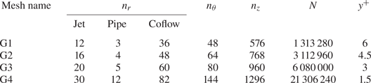
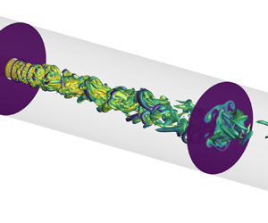
To establish a detailed understanding toward the physics of VVM, an increased grid resolution, G4, is also included in LES simulations. This level of mesh refinement highly resolves the mixing hydrodynamics resulting in negligibly small model-dependent SGS contributions. The mixing structures (see § 3.2), the significance of viscous terms in momentum transport (see § 3.3) and jet laminarization characteristics (see § 3.4) are investigated using this highly resolved LES data.
The inflow condition is found to be critical in determining the early mixing structures and evolution of the shear layer in LES simulations. Initially, the domain is set to start axially right where fluid mix (no upstream section) and the experimental mean flow profiles are applied with added temporal fluctuations that match with desired turbulence statistics. Although this synthetic turbulent inflow condition provides reasonable predictions of the mean flow, the covariance of fluctuating terms shows significant discrepancies. Then the inlet is extended two outer diameters ( $2D=10d$) upstream and the same velocity profiles are applied in anticipation of the developed turbulent structures. It is observed that the predictions are not satisfactorily matching. Finally, a mapping boundary condition defined as
 \begin{equation} \boldsymbol{u}(\boldsymbol{r}_{in},t) = \alpha_m \boldsymbol{u}(\boldsymbol{r}_{in}+8d\,\hat{\!\boldsymbol{i}},t) \end{equation}
is applied to the jet and coflow inlet where  $\hat {i}$ indicates axial flow direction. The solution for a property of interest is interpolated at $8d$ downstream and mapped to the inlet as shown in figure 1. The studies conducted by Kim & Adrian (Reference Kim and Adrian1999) indicate that $8d$ mapping distance encapsulates major coherent turbulent structures. To conserve the inflow rate, the mapped velocity is multiplied by a correction factor, $\alpha _m$, which reads
 \begin{equation} \alpha_m = \frac{Q_{in}}{\iint_\mathcal{S} \boldsymbol{u}(\boldsymbol{r}_{in}+8d\boldsymbol{i},t) \,{\rm d}\mathcal{S}}, \end{equation}
where  $Q_{in}$ is the inlet flow rate and $\mathcal {S}$ is the mapping plane. In the end, a reasonable agreement with experiments is obtained in the mixing chamber. A relevant study on the effect of inlet conditions on predicting the desired flow over a wall-mounted hump suggests the superiority of the plane mapping over a fixed velocity profile and synthetic turbulent inlet (Montorfano, Piscaglia & Ferrari Reference Montorfano, Piscaglia and Ferrari2013). Besides the inflow condition, a no-slip surface condition is imposed on the walls and a pressure outflow boundary condition is applied at the outlet. The same boundary conditions are used for RANS simulations.
Furthermore, the validity of the method is tested by comparing the flow profiles in the upstream jet pipe with DNS solutions of turbulent pipe flow provided by El Khoury et al. (Reference El Khoury, Schlatter, Noorani, Fischer, Brethouwer and Johansson2013). The data reported for  $Re_b=11\,700$, bulk Reynolds number, is used for comparison that is the closest to our problem ( $Re_j=11\,400$). The profiles of mean velocity and the root mean square (r.m.s.) of fluctuations with inner scaling are presented for three LES simulations with varying grid size and DNS in figure 3. Here $y^+$ is defined as $(1-r)^+$ and the velocities are normalized with mean friction velocity, $u_\tau$. The LES are conducted using the dynamic Smagorinsky model as described in the following section. Although there is a discrepancy in $u_r^+$, overall the mapping provides a satisfactory inflow condition and the G2 mesh is found to be acceptable that is consistent with the mesh level selection reported above. This validation study applies to all viscosity ratios as the jet viscosity is the same across.

Figure 3. Radial profiles of mean velocity (a) and the r.m.s. of axial (b), radial (c) and azimuthal (d) velocity fluctuations shown at the upstream jet pipe (between the inlet and mapping plane). Plot (e) depicts the comparison of laminar coflow velocity profile in the same upstream location against analytically obtained velocity profiles using (2.8).
In the disparate viscosity cases, coflow is always laminar and, hence, the velocity profile is analytically obtained as
 \begin{equation} U_x ={-}\frac{{\rm d}p}{{\rm d}x} \frac{1}{4{\rm \pi}} \left[R_i^2 - r^2 + (R_o^2 - R_i^2) \frac{\ln{r/R_i}}{\ln{R_o/R_i}}\right], \end{equation}
where  $R_i$ is the inner radius and $R_2$ is the outer radius. In the analytical solution, no-slip boundary conditions ( $U_x(r|r=R_i) = 0$ and $U_x(r|r=R_o) = 0$) are applied. Figure 3(e) shows this analytically obtained profile and time-averaged LES results using the dynamic Smagorinsky model obtained with the G2 mesh. The matching comparison suggests that LES with the mapping boundary condition accurately reproduces the analytical profile. Also, this result assures the use of LES with dynamic Smagorinsky in laminar flow zones that is observed partially as the jet laminarizes in downstream locations.
2.2.2. Large-eddy simulations
The LES equations are derived by applying a spatial filter to NS equations that separate eddies into resolved and unresolved scales based on the selected filter size. The filtered equations for the flow field and mixture fraction reads
 \begin{gather} \frac{\partial \bar{u}_i}{\partial t} + \bar{u}_j \frac{\partial \bar{u}_i}{\partial x_j} ={-}\frac{1}{\rho} \frac{\partial \bar{p}}{\partial x_i} + \bar{\nu} \frac{\partial^2 \bar{u}_i}{\partial x_j^2} + 2\frac{\partial \bar{\nu}}{\partial x_j} \bar{S}_{ij} - \frac{\partial \tau_{ij}^{LES}}{\partial x_j} + \varGamma_1^{LES} + \varGamma_2^{LES}, \end{gather}
 \begin{gather} \frac{\partial \bar{\xi}}{\partial t} + \bar{u}_i \frac{\partial \bar{\xi}}{\partial x_i} = D \frac{\partial^2 \bar{\xi}}{\partial x_i^2} - \frac{\partial q_i^{LES}}{\partial x_i}, \end{gather}
where  $\bar {u}$ is filtered velocity, $\rho$ is density, $\bar {p}$ is filtered pressure, $\bar {\nu }$ is kinematic viscosity, $\bar {S}_{ij}$ is the filtered strain-rate tensor, $\bar {\xi }$ is the filtered mixture fraction and $D$ is the molecular diffusion coefficient. In the filtered equations the contribution of unresolved scales, subgrid scales (SGS), appears in the following terms where $\tau _{ij}^{LES}$ is the stress tensor, $q_i^{LES}$ is the scalar flux and $\varGamma _1^{LES}, \varGamma _2^{LES}$ are contraction of viscosity and strain-rate tensor. They are defined as
 \begin{gather} \tau_{ij}^{LES} = \overline{u_iu_j} - \bar{u}_i\bar{u}_j,\quad q_i^{LES} = \overline{u_i\xi} - \bar{u}_i\bar{\xi},\end{gather}
 \begin{gather}\varGamma_1^{LES} = \overline{\nu \frac{\partial^2 u_i}{\partial x_j^2}} - \bar{\nu} \frac{\partial^2 \bar{u}_i}{\partial x_j^2},\quad \varGamma_2^{LES} = \overline{\frac{\partial \nu}{\partial x_j} S_{ij}} - \frac{\partial \bar{\nu}}{\partial x_j} \bar{S}_{ij}. \end{gather}
The unclosed SGS stress tensor,  $\tau _{ij}^{LES}$, is formulated in eddy viscosity form that reads $-2\nu _{sgs}\overline {S_{ij}}$. The SGS kinematic viscosity, $\nu _{sgs}$, is locally calculated using three different models with implicit filtering where filter width, $\varDelta$, is defined to be the cube root of the grid volume; Smagorinsky (Smagorinsky Reference Smagorinsky1963), dynamic Smagorinsky (Germano et al. Reference Germano, Piomelli, Moin and Cabot1991) and dynamic $k$ equation (Kim & Menon Reference Kim and Menon1995). In the Smagorinsky model the eddy viscosity is modelled as a function of dimensionless empirical coefficient, $c_s$, length scale, $\varDelta$, and a velocity scale, $\varDelta |\boldsymbol{\mathsf{S}}|$, where $|\boldsymbol{\mathsf{S}}|=\sqrt {2\overline {S_{ij}}\overline {S_{ij}}}$. The dynamic variant of this model proposed by Germano (referred to as dynamic Smagorinsky) applies an explicit filter (top hat), $\alpha \varDelta$, where $\varDelta$ is the SGS filter size and $\alpha >1$ ( $\alpha = 2$ in the present study). Then it seeks a $c_s$ value as a function of space and time determined from the resolved scales. This eliminates the limitations introduced by the constant empirical coefficient approximation. Particularly, having a computational domain of mixed laminar and turbulent regions, dynamic calculation of the model coefficient provides an irrefutable advantage. However, the dynamic calculations are also prone to instabilities due to disparate $c_s$ coefficients at different length scales, large spatial gradients of $c_s$ and division by zero. A more robust calculation that removes the zero-division problem proposed by Lilly (Reference Lilly1992) is implemented that considers volume averaging. Two different models, to close the SGS stress tensor, explained so far are described as algebraic models. The third model used in the present study is a one-equation model, dynamic $k$ equation, that solves a transport equation for SGS TKE to determine eddy viscosity. Kim & Menon (Reference Kim and Menon1995) proposed the dynamic modelling method to the $k$-equation SGS model to adjust model parameters in space and time. One of the significant benefits of a one-equation model over algebraic models is that it relaxes the local equilibrium of TKE production and dissipation assumption so it can account for non-local and history effects.
The SGS turbulent scalar flux,  $q_j^{LES}$, is modelled using the gradient diffusion method that leads to
 \begin{equation} q_j^{LES} ={-} \frac{\nu_{sgs}}{Sc_t} \frac{\partial \bar{\xi}}{\partial x_i}, \end{equation}
where  $\nu _{sgs}$ is SGS kinematic viscosity and $Sc_t$ is the turbulent Schmidt number set to be 0.7.
In the present study the contraction of viscosity and strain-rate tensor terms,  $\varGamma _1^{LES},\ \varGamma _2^{LES}$, are neglected since there are no available SGS closure models. This assumption is justified by the fact that LES solutions obtained by G4 grid size resolve more than 98 % of the energy-containing larger scales such that the contribution of SGS terms remains relatively small. This is quantified by measuring the ratio of SGS turbulence to total turbulence, with a relation given by
 \begin{equation} \phi_k = \frac{k_{sgs}}{k_{sgs}+\bar{k}} . \end{equation}
However, in future studies the validity of this assumption should be tested using model-free direct numerical simulations.
When solving (2.10), 2.15, a multi-dimensional limiter for explicit solution (MULES) algorithm (Deshpande, Anumolu & Trujillo Reference Deshpande, Anumolu and Trujillo2012) is utilized to maintain the boundedness of the mixture fraction field. From the solved field, the kinematic viscosity is corrected, based on (2.2), to be used in the momentum equation. This process satisfies the coupling between momentum and mixture fraction equations. The temporal stability of the LES simulations is ensured with an adaptive time step that limits the flow and interface Courant numbers by 0.35. The equations are discretized using second-order CrankNicolson with a blending coefficient of 0.9 for time integration, a pure second-order van Leer interpolation (Van Leer Reference Van Leer1974) for scalar divergence operations (convective terms) and second-order linear interpolation for Laplacian operations (diffusive terms). The simulations are conducted in OpenFOAM-v6 (an open-source, cell-centred finite volume solver) using ‘twoLiquidMixingFoam’ solver. This specific solver is designed for mixing two miscible incompressible fluids with disparate viscosity.
The temporal sampling frequency and duration of LES simulations are decided based on the eddy-turnover time,  $t_e$, and flow through time, $t_f$. With the flow parameters and domain given in this study, $t_e$ and $t_f$ are calculated as 0.26 s and 2.6 s, respectively. The simulations, using four Skylake (SKX) nodes (192 CPU cores) of TACC's Stampede2 HPC system, run for 23 $t_f$ (230 $t_e$) and during this period $1200$ instantaneous samples (weak temporal correlation between consecutive samples) are collected. Subsequently, the first- and second-order statistics are obtained based on the ensemble average of the instantaneous solutions, and convergent mean and fluctuating quantities are confirmed. The computational demand of each simulation with G2 and G4 meshes is determined to be ${\approx }18\,000$ and ${\approx }550\,000$ CPU hours.
A direct comparison of a scalar field, i.e. mixture fraction, predictions between LES and PLIF field measurements requires one to take the planar laser sheet thickness into account. In the experimental set-up the planar sheet thickness is 1 mm so that the resultant PLIF measurement is a spatial average across this length. Although the effect is negligible in the mean field, it is discernible in the scalar variance field. To account for this, instantaneous LES predictions are extracted and averaged over the same thickness. Then  $1200$ adjusted snapshots are averaged to calculate the mean and variance of the mixture fraction.
2.2.3. Reynolds-averaged Navier–Stokes
Steady RANS equations are obtained by decomposing a property into mean and fluctuating components ( $\phi = \left \langle \phi \right \rangle + \phi '$) and averaging for a certain period of time that leads to a time-independent mean $\left \langle \phi \right \rangle$ and zero-mean fluctuations, $\langle \phi '\rangle =0$. The RANS equation for variable viscosity and Reynolds-averaged AD equation reads
 \begin{gather} \left\langle u_j\right\rangle\frac{\partial\left\langle u_i\right\rangle}{\partial x_j} ={-}\frac{1}{\rho} \frac{\partial \left\langle p\right\rangle}{\partial x_i} + \left\langle\nu\right\rangle \frac{\partial^2 \left\langle u_i\right\rangle}{\partial x_j^2} + 2\frac{\partial \left\langle\nu\right\rangle}{\partial x_j}\left\langle S_{ij}\right\rangle + \frac{\partial \tau_{ij}^{RANS}}{\partial x_j} + \varGamma_1^{RANS} + \varGamma_2^{RANS}, \end{gather}
 \begin{gather} \left\langle u_i\right\rangle \frac{\partial \left\langle\xi\right\rangle}{\partial x_i} = D \frac{\partial^2 \left\langle\xi\right\rangle}{\partial x_i^2} - \frac{\partial q_i^{RANS}}{\partial x_i}, \end{gather}
where quantities denoted with  $\left \langle \bullet \right \rangle$ corresponds to time-averaged properties, $\left \langle u \right \rangle$ is mean velocity, $\rho$ is density, $\left \langle p \right \rangle$ is mean pressure, $\left \langle \nu \right \rangle$ is mean kinematic viscosity, $\left \langle S _{ij}\right \rangle$ is the mean strain-rate tensor, $\left \langle \xi \right \rangle$ is the mean mixture fraction, $D$ is the molecular diffusion coefficient, $\tau _{ij}^{RANS}$ is the Reynolds stress tensor and $q_i^{RANS}=\left \langle u _i' \xi '\right \rangle$ is the turbulent scalar flux. The additional closure terms, $\varGamma _1^{RANS},\ \varGamma _2^{RANS}$, that arise from the decomposition of viscosity fluctuations represent the mean contraction of viscosity and strain-rate tensor. They are given by
 \begin{equation} \varGamma_1^{RANS} = \left\langle\nu'\frac{\partial^2 u_i'}{\partial x_j^2}\right\rangle,\quad \varGamma_2^{RANS} = \left\langle2\frac{\partial \nu'}{\partial x_j} S_{ij}'\right\rangle, \end{equation}
where quantities denoted with  $\bullet '$ corresponds to the fluctuation of properties about mean values, $\left \langle \bullet \right \rangle$. The local viscosity is calculated based on the linear scaling given in (2.2).
The Reynolds stress term, shown with  $\tau _{ij}^{RANS}=-\left \langle u _i' u_j'\right \rangle$ in (2.14), is closed using the linear eddy viscosity model that postulates a linear relationship between the deviatoric part of Reynolds stress and mean strain-rate tensor, which reads
 \begin{equation} -\left\langle u_i' u_j'\right\rangle=2 \nu_t \left\langle S_{ij}\right\rangle - \frac{2}{3}k\delta_{ij}, \end{equation}
where  $\nu _t$ is a proportionality constant. In the current study this proportionality constant, the kinematic eddy viscosity, is calculated using two different two-equation RANS models; $k-\epsilon$ (Launder & Spalding Reference Launder and Spalding1974) and $k-\omega$ SST (Menter, Kuntz & Langtry Reference Menter, Kuntz and Langtry2003).
In the  $k-\epsilon$ model the expression for kinematic eddy viscosity takes the form $\nu _t=C_{\mu } k^2 / \epsilon$, where $\epsilon$ is the total rate of dissipation. Two separate transport equations are solved for $k$ and $\epsilon$ with the model coefficients of $C_{\mu }=0.09$, $C_1=1.44$, $C_2=1.92$, $\sigma _k=1.0$ and $\sigma _{\epsilon }=1.3$ as described in Launder & Spalding (Reference Launder and Spalding1974, table 2.1).
In the  $k-\omega$ SST model the expression for kinematic eddy viscosity takes the form $\nu _t = a_1 k / \max {a_1 \omega, b_1 F_{23} S}$, where $F_{1}$ is the blending function that ensures a proper selection of $k-\omega$ and $k-\epsilon$ zones based on wall distance. Two separate transport equations are solved for $k$ and $\omega$ with the model coefficients of $\alpha _{k1}=0.85$, $\alpha _{k2}=1.0$, $\alpha _{\omega 1}=0.5$, $\alpha _{\omega 2}=0.856$, $\beta _1=0.075$, $\beta _2=0.0828$, $\beta ^*=0.09$, $\gamma _1=5/9$, $\gamma _2=0.44$, $a_1=0.31$, $b_1=1.0$ and $c_1=10.0$ as described in Menter et al. (Reference Menter, Kuntz and Langtry2003).
To close the turbulent scalar flux term,  $q_i^{RANS}=\left \langle u _i' \xi '\right \rangle$, the gradient diffusion method is employed and it is given by
 \begin{equation} q_i^{RANS} ={-} \frac{\nu_t}{Sc_t} \frac{\partial \left\langle\xi\right\rangle}{\partial x_i}, \end{equation}
where  $\nu _t$ is turbulent kinematic viscosity and $Sc_t$ is the turbulent Schmidt number set to be 0.7. This hypothesis requires co-alignment between turbulent scalar flux and mean scalar gradient that is evaluated using highly resolved LES data (see § 3.3).
In the RANS simulations the contraction of viscosity and strain-rate tensor terms,  $\varGamma _1^{RANS},\ \varGamma _2^{RANS}$, are also neglected. Based on the time-dependent flow field and mixture fraction predictions provided by highly resolved LES, described in the following subsection, we observe that these terms are significant to remain unclosed (see § 3.3), especially in the early mixing regions. However, in the current study the intention is to evaluate the performance of available standard RANS models on the mixing of fluids with disparate viscosity. Since there is no adequate model to close terms shown in (2.16a,b), to the best of the authors’ knowledge, these terms are neglected in the solution.
The RANS simulations solve three-dimensional steady-state partial differential equations for the velocity and mixture fraction shown in (2.14) and (2.15), in addition to solving the Poisson equation for pressure to satisfy the continuity. For convective and diffusive terms, the same discretization schemes are used as for the LES. For the pressure equation, the relaxation factor is 0.3 while, for the remaining equations, the value is 0.7. The absolute residual tolerance for the pressure equation is  $10^{-8}$ while, for all of the other variables, it is $10^{-7}$. The simulations run on one Skylake (SKX) node (48 CPU cores) of TACC's Stampede2 HPC system where a convergent solution is reached at around 6000 iterations. Each simulation with the G2 mesh demands ${\approx }2000$ CPU hours.
2.3. Experiments
The experiments were performed in the viscous mixing jet facility at the Georgia Institute of Technology. This is a pressure-driven, modular facility capable of sustaining aqueous flows with viscosity disparities of the order of 1000 Pa s. The facility was configured to match the co-annular test geometry used in this study.
A schematic of the facility is shown in figure 4. As shown, test fluids are prepared in 900 l mixing tanks, then transferred into 800 l driving tanks. Both inner and outer fluids are water. In the preparation the outer flow viscosity is increased by mixing the water-soluble viscosity modifier (sodium carboxymethylcellulose) where the mixture remains Newtonian at the concentration and shear rates considered in this study. The experiments are conducted in a temperature-controlled lab space with a  $2\,^\circ {\rm C}$ characteristic drift. The actual temperature fluctuations inside the tank were found to be an insignificant fraction of $2\,^\circ {\rm C}$ that assures to decouple dynamic viscosity from the temperature effect. The fluids are pumped with a steady back pressure of pressure-regulated nitrogen and throttled by high flow rate control valves (Fisher 2-inch 24000SVF-54-3661) controlled by the readings of inline ultrasonic flow meters (Omega FDT-40). The flows are conditioned in a settling chamber where the outer flow is directed through a series of honeycombs and meshes in a circular cross-section with 16 times the area as the test section. The inner flow travels through a 10 mm section of 75 diameters before entry into the test section to ensure a fully developed turbulent pipe flow. Simultaneous PIV and PLIF are performed in the 1.5 m optically accessible test section to observe the concurrent velocity and concentration fields. The acquisition system, shown in figure 4, mounts two cameras (29 MP TSI Powerview) on an assembly that can translate to observe adjacent areas of the flow field. The flow field is illuminated by 120 mJ laser pulses (Litron Nano-PIV 532 nm) that pass through a series of lenses to form a 1 mm sheet through the centre of the pipe. Operating at 1 Hz, both of these cameras observe a $50\,{\rm mm} \times 80\,{\rm mm}$ domain corresponding to a $1D \times 1.6D$ acquisition region, where they record 250 realizations of the turbulent flow field at each streamwise location. The camera resolution enables roughly $5 \lambda _{K}$ PIV resolution and $10 \lambda _{B}$ PLIF resolution in a plane over the domain, enabling high-resolution velocity and concentration measurements over the full extent of the pipe. Using this acquisition system, the experiments observe the first $6.4D$ of the flow field.

Figure 4. Schematic of the experimental facility.
Planar laser-induced fluorescence was employed with Rhodamine 6G ( $1.85\times 10^{-5}\, {\rm kg}\,{\rm m}^{-3}$) seeded into the outer stream. This enabled PLIF calibration to be performed during testing by running only the outer flow and observing a pure Rhodamine field at every test domain. The PLIF camera was fitted with a notch filter to remove the 532 nm PIV signal (6 nm FWHM). The PLIF fields were post processed in MATLAB with self-developed codes by current authors and it is described in Pathikonda et al. (Reference Pathikonda, Usta, Ahmad, Khan, Gillis, Dhodapkar, Jain, Ranjan and Aidun2021). Particle image velocimetry was implemented using hollow glass microspheres (Potters beads characteristic size $25\,\mathrm {\mu }{\rm m}$) mixed into both streams. These microspheres were calculated to have a Stokes response time of $35\,\mathrm {\mu }{\rm s}$ and were therefore trusted to follow the smallest scales of the velocity field. The glass microspheres were illuminated by the double-pulsed laser with 250 ms between pulses. The PIV fields were post processed in LaVision Davis 8.4 with $24\times 24$ pixel resolution and 50 % overlap, resulting in greater than 97 % of vectors satisfying outlier criteria. To characterize the uncertainty of PIV and PLIF measurements, central limit theorem is applied. With a 95 % confidence interval, the uncertainty of the population means is obtained ${\approx }2\,\%$ whereas this number is ${\approx }14\,\%$ for the uncertainty of the variance. Further details on PIV and PLIF post processing are given in Pathikonda et al. (Reference Pathikonda, Usta, Ahmad, Khan, Gillis, Dhodapkar, Jain, Ranjan and Aidun2021) and Ahmad (Reference Ahmad2021).
3. Results and discussions
3.1. Comparison and analysis of velocity and mixture fraction
In this subsection the performance of predictions acquired by three LES and two RANS models, using the G2 mesh, are compared against experimental measurements reported by current authors (Pathikonda et al. Reference Pathikonda, Usta, Ahmad, Khan, Gillis, Dhodapkar, Jain, Ranjan and Aidun2021) for the lowest (m1) and highest (m40) viscosity ratios. In figures 5–8 radial profiles of quantities of interest are presented for m1 in the top row and m40 in the bottom row. The profiles are plotted at three distinct streamwise locations that are  $x/D = 0.5$, $2$ and $5$, where $D$ is the outer diameter. Although the quantities of interest obtained with each method are shown with different notations (LES, $\bar {\bullet }$; RANS, $\left \langle \bullet \right \rangle$; and Exp, $\bullet$), they are simply represented with no overline or brackets.

Figure 5. Evolution of radial profiles of mean velocity rendered at three different streamwise locations for m1 (a–c) and m40 (d–f). The profiles are normalized by the bulk velocity,  $U_p$.

Figure 6. Evolution of radial profiles of axial velocity fluctuations r.m.s. rendered at three different streamwise location for m1 (a–c) and m40 (d–f).

Figure 7. Evolution of radial profiles of the mean mixture fraction rendered at three different streamwise locations for m1 (a–c) and m40 (d–f). The profiles are normalized by the centreline mixture fraction,  $\xi _0$.

Figure 8. Evolution of radial profiles of mean mixture fraction fluctuations rendered at three different streamwise locations for m1 (a–c) and m40 (d–f).
Figure 5 shows the mean axial velocity normalized by the bulk velocity,  $U_p$, given in table 1. The jet expansion predicted by the Smagorinsky model is underestimated in the early locations while it is overpredicted in downstream locations. This indicates that the constant model coefficient accurately governs the evolving mixing physics neither in m1 nor m40. The dynamic LES models adjust to capture the local mixing conditions, thereby offering a great agreement with the experimental data throughout the mixing chamber. On the contrary, even though RANS predictions indicate a certain level of agreement in the first two locations, it deviates notably later in both cases. Considering m1 has no variable-viscosity physics, the discrepancy with experiments stems from the inability of the RANS closure model in predicting the energy production due to the K–H-type instabilities. Furthermore, to shed light on the applicability of well-known energy cascade scaling in the inertial subrange, the energy spectrum is plotted and discussed in the following subsection (see figure 23). In m40, RANS predictions deviate even more in the last locations. This is envisaged since the turbulence model becomes ill-defined in the unsteady laminar region and it behaves severely dissipative as if the turbulence momentum diffusion is dominant. More evidence on the existence of unsteady laminar flow is discussed in figure 23.
The profiles in near jet entry, shown in figure 5(a,d), illustrate the noteworthy shear between the jet and coflow interface that manifest as well-known K–H waves. While K–H instabilities are key in inducing initial perturbation of the shear layer interface, later it transitions to a more complex three-dimensional system. On top of it, viscosity variations induce additional instabilities. Particularly in m40 the entrainment between the inner and outer flow, stemming from K–H and viscosity gradient instabilities, dictates the local viscosity and its gradients. Consequently, the increased local viscosity in the shear layer increases momentum diffusion while decreasing the local Reynolds number. When m1 and m40 velocity profiles at  $x/D=2$ are compared, higher local velocities, hence elevated momentum diffusion, are observed in the shear layer between $0.2< r/D<0.3$ in m40. This observation also means that the shear velocity, driving the K–H instabilities, is less in the higher viscosity. Ultimately, the velocity profiles transition towards fully developed turbulent flow in m1 and laminar flow in m40.
The root-mean-squared values of streamwise velocity fluctuations obtained with LES and experiments are presented in figure 6. In the first two axial locations the Smagorinsky model overpredicts the fluctuations and this is consistent with the findings on the higher jet expansion rates predicted by this model discussed above. As seen in figure 6(a–c), the dissipative nature of the Smagorinsky model, arising from spurious eddy viscosity stem from the mean shear, result in decaying turbulence activity at the near wall that is an unphysical solution according to the wall-bounded turbulence theory. Although there are wall-damping methods available to alleviate these deficiencies, the standard method is purposely tested since we intend to predict the shear layer evolution.
In m40 (TLL), the pipe flow eventually transitions to steady laminar flow as determined a priori by the equilibrium flow rate and viscosity. However, the non-zero r.m.s. of fluctuations in the interrogated axial locations indicates a transitional flow regime in the form of unsteady laminar flow that lasts for several diameters. An unsteady laminar flow assertion is also verified by decaying turbulence activity near the wall in figure 6(f). On the contrary, m1 shows an increase in the magnitude of near-wall fluctuations and the overall agreement in the shear layer and near-wall region between dynamic LES models and PIV proves the validity of these models.
Figure 7 presents the mean mixture fraction normalized by the mean centreline value,  $\xi _0$. The drawbacks of the Smagorinsky model mentioned earlier are evident in the mixture fraction evolution. The overpredicted velocity fluctuations (see figure 6) induce turbulent scalar flux resulting in an overestimation of jet expansion. However, the dynamic LES models used in this study provide an excellent comparison against PLIF. The accuracy of mixture fraction predictions is particularly important in this study since they indicate accurate modelling of the two-way coupled VVM physics.
The quality of RANS predictions relies heavily on the validity of the closure models selected for the Reynolds stress and concentration fields. Seeing as the principles underlying these closures have not been validated in a disparate viscosity context, these simulations represent the best of current practices for CVM. Along the same line of discussion in figure 5, RANS overpredicts the jet spreading in general. However, the severity of the discrepancy is pronounced in the last location. Reynolds-averaged Navier–Stokes suggests almost a complete homogenization of fluids that is quite contradictory to experiments and LES. One noteworthy aspect of the RANS predictions is that the jet width is quite similar between m1 and m40. It appears that the model is incapable of capturing differing shear layer evolutions discussed in the following subsection (see figure 9).

Figure 9. Interfacial dynamics of a turbulent jet issued into a coflow with equal ( $m=1$) and variable ( $m=10$, $20$,
$20$,  $40$) viscosity ratio. The isosurfaces are rendered at equilibrium mixture fraction, $\xi _{eq} = 0.2$.
Particularly in m40, having a scalar transport through a TNTI and jet laminarization adds more complexity. In the mixing zones, the stark difference between TTT and TLL and jet laminarization in TLL are pronounced. The dynamic LES models resolve all the scales in this transitioning unsteady region since the contribution of unresolved eddies conspicuously decays to negligible levels by  $x/D\geq 2$. Apparently, the likely cause of the discrepant predictions by the Smagorinsky model discussed earlier, is the inadequacy of using a constant model coefficient in the transitioning region. In addition to omitting variable-viscosity closure terms, the RANS computation also misses physics in the transition to a laminar regime since the entire domain is simulated with the same model.
It is anticipated that the real difference would be observed in the r.m.s. of mixture fraction fluctuations that have key importance in many processes including fast chemical reactions. Figure 8 plots the variance of mixture fractions that are resolved in LES. Here, there are no data points pertaining to RANS because no transport equation or algebraic calculations are employed in this study. Through a similar argument as before, in general, the Smagorinsky model deviates and, particularly at  $x/D=0.5$, both the width and magnitude of the fluctuating region are discrepant with experimental data. On the other hand, dynamic LES models pronounce the advantage of locally adjusted model coefficients by the agreement with experimental data, given that it has 14 % measurement uncertainty, in both early and downstream locations.
The magnitude of fluctuations in the downstream locations is a good indication to assess the level of unmixedness of the jet, such that it should be zero in the fully mixed region. In general, m40 attains higher magnitudes of fluctuations due to large pockets of unmixed ‘blobs’ described as folded-segregated structures (see figure 11). Specifically, the decay of fluctuations downstream in m40 happens slowly when compared with m1. This behaviour suggests that the flow is already transitioned to unsteady laminar (as evidenced in the discussion of figure 6( f)) at  $x/D=5$ so that the lack of turbulent eddies manifests itself as prolonged unmixed regions.
Overall, in this section it is shown that dynamic LES models using the medium-level mesh (G2) provide satisfactory results when compared with PIV and PLIF measurements whereas standard RANS models fail noticeably. To understand mixing physics at disparate viscosity conditions and investigate the effect of unclosed terms arising from variable viscosity in RANS equations, the remainder of the results and discussions utilize highly resolved LES data obtained by G4 grid resolution that minimizes the SGS model dependency. Especially in the variable-viscosity cases, this mesh provides a DNS-like solution since elevated viscosity reduces the effective Reynolds number.
3.2. Development of jet interface in TTT and TLL mixing modes
Figure 9 shows the snapshot of the interfacial dynamics of TTT (m1) and TLL (m10, m20, m40) cases for qualitative analysis. As fluids are miscible, the level of isosurfaces is set to 0.2, which is the equilibrium mixture fraction based on the inlet condition. In all cases, although the interface expands to similar diameters at the given distance, a discernible difference in interfacial dynamics is observed between TTT and TLL cases. In m1 the shear layer instabilities grow rapidly and break the axis symmetry almost immediately after jet injection. Then the flow becomes three dimensional, leveraging the azimuthal mixing mechanism that limits the formation of ‘mushroom’-like larger structures. This phenomenon elucidates the formation of small-length scale structures that generate this intricate interface. It is apparent that shear-driven TKE production is initiated by K–H-type instabilities that promote early mixing. This is also evident in energy spectra that in early mixing K–H instabilities inject a range of TKE that causes deviation from  $-5/3$ in the inertial range. Therefore, we can conclude that the TTT mixing mode leads to rapid homogenization of fluids at the shear layer and limited entrainment through larger structures.
In TLL cases one should also consider the Yih-type instabilities due to viscosity stratification in addition to K–H instabilities for a complete discussion. In the scope of the current study, it is not directly possible to decouple these two instabilities. However, having different viscosity ratios in TLL and TTT cases with matching inlet momentum enables us to investigate the overall effect of viscosity variations on interface development. Overall, the interfacial waves engulf large pockets of outer fluid into the centreline in early locations but the mixing mechanism dispersing these structures after engulfment is limited by laminarization caused by elevated viscosity. The mechanisms generating interfacial waves in the azimuthal direction decay. Without mechanisms to further generate the interfacial area, the previously formed waves persist in a folded-segregation pattern. The unsteady laminar flow shears these waves into semi-toroidal sheet-like structures. When comparing cases from m10 to m40 with increasing viscosity ratio, we observe that the entrainment of jet to coflow is suppressed and the interface is less disturbed in the azimuthal direction that results in an even larger unmixed fluid parcel. It is interpreted that increasing viscosity laminarizes the jet faster leading to less vortical activity to induce mixing.
To support these observations, figure 10 renders isosurfaces of normalized Q criterion for TLL cases. Isosurfaces are also coloured with mixture fractions so that we can conveniently identify zonal vortical activity between the jet and coflow. The difference in axisymmetry break is so distinct in early locations,  $0 < x/D < 1$. In m1 coherent vortical structures indicate that the shear layer is three dimensional throughout whereas in the other two cases we can identify initial coherent vortex rings ( $0 < x/D < 0.5$; pointed with dashed arrows) that remain almost intact in a circular shape. This shows the dominant effect of flow laminarization due to increasing viscosity when compared with instabilities triggered by viscosity stratification. This is also evident in rapid vortical structure decay in m40, whereas we observe ‘volume-filling’ vortical activity in m10. Also, the size of the vortices (see solid arrows) is increasing with the increasing viscosity ratio, which indicates the coarsening effect of lowering the effective Reynolds number. When the vortical activity is analysed in early locations, $0 < x/D < 2$, it is clear that at lower viscosity ratios immediate axisymmetry break and a relatively higher effective Reynolds number lead to higher rates of vortical expansion in the radial direction. These qualitative observations reveal that increasing the viscosity ratio (so overall viscosity) stabilizes the flow more so than viscosity stratification instabilities.

Figure 10. Isosurfaces of normalized Q criterion (Q $D^2 / U_b^2 = 60$) shown for m10 (a), m20 (b) and m40 (c). Isosurfaces are coloured with the mixture fraction where $\xi =1$ for the jet and $\xi = 0$ for the coflow. The grey shade in the background of each panel depicts the computational domain.
To elucidate the difference between the homogenized mixing layer and folded-segregated patterns, the evolution of the mixture fraction is demonstrated at longitudinal and cross-sectional planes in figure 11. The stark difference between TTT and TLL is attributed to different mixing modes. In the viscosity matched case, m1, both the jet and coflow are turbulent and they transition to a fully developed turbulent pipe flow downstream. However, in the higher viscosity ratios, while the jet flow is turbulent, the coflow and downstream pipe remain in the laminar regime due to the increased viscosity. This condition introduces a TNTI phenomena in the early locations of the developing mixing layer. The spatiotemporal evolution of the TNTI is dictated not only by nature mixing but also by the presence of a viscosity gradient in the first place. As two miscible fluids entrain at the interface, the magnitude of the viscosity gradients decreases and ultimately disappears when the mixing reaches equilibrium. Hence, in the regions where viscosity fluctuations and TNTI are significant, the model needs to encapsulate a closure for the effects of both viscosity gradients as well as momentum transport at the TNTI. Inherently, LES offers several advantages over RANS-type models since most energy-containing fluctuations are resolved and the SGS turbulence level is adjusted dynamically to account for TNTI.

Figure 11. Evolution of the instantaneous mixture fraction shown across the flow with centreplanes and eight different cross-sectional planes for  $m=1$, $10$,
$10$,  $20$,
$20$,  $40$ from (a–d). The contours are overlaid with half-mixing, $\xi _h=0.5$ (black) and equilibrium mixing, $\xi _{eq}=0.2$ (white) isolines. The cross-sectional planes for each viscosity ratio are depicted at $x/D = 0.5$, $1$,
$1$,  $2$,
$2$,  $3$,
$3$,  $4$,
$4$,  $5$,
$5$,  $6$ and $8$ from left to right.
The spatial distribution of the mixture fraction at subsequent cross-sectional planes indicates the increased level of non-axisymmetry and intricacy of the interface in TLL. In TTT, overall, the circular-like shape of the jet remains intact for longer distances and the probability of observing the pure outer fluid at the centreline is very low. However, in TLL, the jet starts to be highly skewed at  $x/D=1$ and it subsequently transitions to the formation of folded-segregated structures. Soon after, the laminar stretching and prolonged existence of the larger pockets of fluids are observed. Especially in m40, pockets of unmixed fluid greater than half-mixing ( $\xi >0.5$) are observed at $x/D=6$. At this pipe location, evidently, the turbulent scalar flux is already decayed to insignificant levels that only shear-driven mixing and relatively slower molecular diffusion mechanisms remain to stir fluids.
The effect of viscosity ratio among TLL cases manifests itself as noticeable differences in both early mixing and further downstream locations. At  $x/D<2$, m10 exhibit more penetrative behaviour meaning that small pockets of jet fluid are detached (see dashed circles) by the induced shear instabilities and are convected into the outer fluid. However, with the increasing viscosity ratio, this detachment phenomenon occurs at later axial locations. This is well explained by the difference in level and coherent structure of vortical activities along the shear layer, as discussed in figure 10. Even the positive correlation between the size of detached jet fluids and vorticity supports this argument. This also provides further evidence about the dominance of shear instabilities over viscosity gradient instabilities that is further discussed in § 3.4.
In the current coaxial confined turbulent mixing setting, the direction of the mean pressure gradient flips several times along the pipe centreline. One observes a favourable pressure gradient (FPG) in the flow direction from the jet outlet to the merging of shear layers. Then, until transitioning to a pipe flow an adverse pressure gradient (APG), where the mean pressure gradient is in the opposite direction of the mean velocity gradient, decelerates the flow. Ultimately in the developed pipe region, FPG is registered. The effect of well-known APG on the mixture fraction structures is distinguishable in m40. As shown in figure 11, the snapshot of mixture fraction for m40 in the longitudinal plane indicates that the shape of the unmixed blobs is more oblate than stretched in the flow direction from  $x/D = 2$ to $5$. Axially decelerating blobs tend to expand in the radial direction. The observations can be described as the development of interfacial waves as well as the formation of mushroom-like structures, resulting in promoted entrainment between the inner and outer flow. This effect is less obvious with the decreasing viscosity ratios.
To unravel the mixing dynamics further, the normalized probability density function (p.d.f.) of the mixture fraction is presented along the centreline ( $r=0$) and centre of the shear layer ( $r=0.5d$) in figures 12 and 13, respectively. The p.d.f.s are centred by the mean and normalized where the approach flows are traced with $\xi _{jet}=1$ and $\xi _{coflow}=0$. Thus, $\xi ^*<0$ indicates outer flow whereas $\xi ^*>0$ indicates inner flow. In m1 the distribution of mixture fraction follows always a Gaussian trend regardless of radial or axial location in the mixing chamber. This behaviour can be intuitively explained by the TTT mixing mode where flow is always turbulent across the domain such that scalar structures are homogenized to equilibrium by the induced flow. However, TLL cases show a different scalar distribution behaviour.

Figure 12. Probability density function (p.d.f.) of the normalized mixture fraction,  $\xi ^* = (\xi - \left \langle \xi \right \rangle )/\xi '_{rms}$, at $x/D=2$ (a), $x/D=4$ (b), $x/D=6$ (c) and $x/D=8$ (d) for m1, m10, m20 and m40. Data are collected along the centreline, $r/d=0$. The normal distribution is shown with dashed grey lines.

Figure 13. Probability density function (p.d.f.) of the normalized mixture fraction,  $\xi ^* = (\xi - \left < \xi \right >)/\xi '_{rms}$, at $x/D=2$ (a), $x/D=4$ (b), $x/D=6$ (c) and $x/D=8$ (d) for m1, m10, m20 and m40. Data are collected along the centre of the shear layer, $r/d=0.5$. The normal distribution is shown with dashed grey lines. In (a) and (b), insets show out-of-range values. For symbol legends, see figure 12.
Along the centreline ( $r/d=0$), m10 and m20 exhibit a negative skew-normal distribution, where the distribution mode is on the inner fluid side, at $x/D=2$, $4$ and $6$. At $x/D=8$ all of the distribution curves collapse to normal distribution regardless of viscosity ratio or mixing mode. However, m40 behaves differently than other TLL cases in $x/D\leq 6$. At $x/D=2$, similar to other TLL cases, negative skew distribution is noted whereas, at $x/D=4$ and $6$, it reveals a bimodal distribution with the new mode peak at the outer fluid side, $\xi ^*<0$. This shows that engulfed and entrained outer fluid reaching to the centreline does not necessarily break down, which suggests that an elevated viscosity ratio quickly decays turbulence even at $x/D=4$. Then laminarization phenomenon prevails so that the dispersion and dissipation mechanism remains limited resulting in persistent scalar fluctuations for longer pipe lengths. It is deduced that in m10 and m20, jet laminarization is delayed so that no pure outer fluid is observed along the centreline. Energy spectra shown in figure 23 corroborates delayed laminarization with decreasing viscosity.
Along the centre of the shear layer ( $r/d=0.5$), m40 is negatively skewed with a persistent bimodal distribution in $x/D\leq 6$, similar to centreline analysis but with a greater magnitude of the peak. Unlike centreline behaviour, m20 is also bimodal at $x/D=2$ and $4$. This type of bimodal distribution is not clearly observed in m10 even though a non-zero distribution density is registered on the outer fluid side at $x/D=2$. Eventually, all curves collapse to normal distribution similar to the centreline location. Therefore, this study reveals that TLL cases exhibit anisotropic scalar distribution either with or without bimodal behaviour up to $x/D=6$. Unless modelled properly, standard RANS models are doomed to fail in predicting scalar distribution accurately.
3.3. Momentum budget analysis of viscous terms
Viscosity variations alter the momentum field that ultimately affects the mixing dynamics. Using highly resolved LES data, we quantify this effect by examining the budgets of the mean momentum equation that includes two additional terms pertaining to the decomposition of viscosity fluctuations. Having a DNS-like grid resolution (G4 mesh) ensures minimal (less than one order of magnitude) contribution from SGS terms. Starting with the highly resolved spatiotemporal flow and mixture fraction field obtained by LES, we decompose a property into LES-resolved mean and LES-resolved fluctuating components  $(\bar {\phi } = \left \langle \bar {\phi }\right \rangle + \phi '')$ and perform a temporal averaging over all available time steps (1200 time steps spanning 23 $t_f$ or 230 $t_e$) that satisfies temporal convergence. With this decomposition, the time-averaged momentum equation reads
 $$\begin{align} \underbrace{\left\langle\bar{u}_j\right\rangle\frac{\partial\left\langle\bar{u}_i\right\rangle}{\partial x_j}}_{\substack{\mathcal{C}}} &= \underbrace{-\frac{1}{\rho} \frac{\partial \left\langle\bar{p}\right\rangle}{\partial x_i}}_{\substack{\mathcal{P}}} + \underbrace{\left\langle\bar{\nu}\right\rangle \frac{\partial^2 \left\langle\bar{u}_i\right\rangle}{\partial x_j^2}}_{\substack{\mathcal{D}_{\bar{\nu}}}} + \underbrace{2\frac{\partial \left\langle\bar{\nu}\right\rangle}{\partial x_j}\left\langle\bar{S}_{ij}\right\rangle}_{\substack{\mathcal{D}_{\boldsymbol{\nabla} \bar{\nu}}}}\nonumber\\ &\quad + \underbrace{\left\langle\nu''\frac{\partial^2 u_i''}{\partial x_j^2}\right\rangle}_{\substack{\mathcal{D}_{\nu''}}} + \underbrace{\left\langle2\frac{\partial \nu''}{\partial x_j} S_{ij}''\right\rangle}_{\substack{\mathcal{D}_{\boldsymbol{\nabla} \nu''}}} - \underbrace{\frac{\partial \left\langle u_i'' u_j''\right\rangle}{{\partial x_j}}}_{\substack{\mathcal{S}}}, \end{align}$$
where quantities denoted with  $\left \langle \bar {\bullet }\right \rangle$ correspond to LES-resolved, time-averaged properties; $\left \langle \bar {u}\right \rangle$ is mean velocity, $\rho$ is density, $\left \langle \bar {p}\right \rangle$ is mean pressure, $\left \langle \bar {\nu }\right \rangle$ is mean kinematic viscosity, $\left \langle \bar {S}_{ij}\right \rangle$ is the mean strain-rate tensor and $\left \langle u _i'' u_j''\right \rangle$ is the resolved stress tensor.
In this subsection we analyse the magnitude and orientation of viscous terms,  $\mathcal {D}_{\bar {\nu }}$, $\mathcal {D}_{\nu ''}$, $\mathcal {D}_{\boldsymbol {\nabla } \bar {\nu }}$ and $\mathcal {D}_{\boldsymbol {\nabla } \nu ''}$. Figures 14, 15, 17 and 18 show radial profiles of radial and axial components at six different axial locations. Solid lines refer to mean terms ( $\mathcal {D}_{\bar {\nu }}$, $\mathcal {D}_{\boldsymbol {\nabla } \bar {\nu }}$) whereas dashed lines represent their fluctuating counterparts ( $\mathcal {D}_{\nu ''}$, $\mathcal {D}_{\boldsymbol {\nabla } \nu ''}$). Note that the centre of the shear layer, $r_s$, is at $r_s=r/D\approx 0.1$, which is important to follow especially when analysing early mixing locations.

Figure 14. Radial profiles of the axial component of  $\mathcal {D}_{\bar {\nu }}$ (solid line) and $\mathcal {D}_{\nu ''}$ (dashed line) terms in (3.1). Profiles are shown at $x/D=0.5$ (a), $x/D=1$ (b), $x/D=2$ (c), $x/D=3$ (d), $x/D=4$ (e) and $x/D=5$ (f) for m10, m20 and m40.


Figure 14 shows the axial component of  $\mathcal {D}_{\bar {\nu }}$ and $\mathcal {D}_{\nu ''}$. At early locations the mean term shows bimodal behaviour with a clear inflection about $r_s$ and later it transitions to a centre-peak profile. This occurs because the turbulent jet is transitioning to a fully developed Poiseuille flow that experiences axial velocity gradients. The fluctuating term peaks at about $r_s$ with a zero centreline value at initial locations and then transitions to a centre-peak behaviour as well. A zero value is intuitive as mixing is not reached to the centreline at early locations. Although the magnitude of fluctuating terms at the peak is less but comparable to their mean counterpart, it shows a more uniform profile along the radial direction, particularly further downstream. Overall, the magnitudes of each term strongly scale by the mean viscosity but such normalization is omitted as it does not collapse exactly. Further normalization is required in future studies.
Interestingly, in  $x/D\leq 1$ mean and fluctuating terms have opposing momentum directions at the outer side of $r_s$. The particular behaviour is actually the key factor that drives K–H-type shear instabilities such that there exists a sharp radial gradient of axial velocity. The flow accelerates on the outer side of the shear layer, $r>r_s$, and it decelerates on the inner side, $r< r_s$, which causes the opposing momentum directions. The strong scaling of peak values with local mean viscosity corroborates this argument. Since the fluctuating term does not exhibit such behaviour, the gradient diffusion based method with isotropic diffusion can not capture this behaviour so solving a separate equation with a non-local model could hope to reproduce this behaviour.
Figure 15 shows the radial component of  $\mathcal {D}_{\bar {\nu }}$ and $\mathcal {D}_{\nu ''}$. On contrary to the axial component, the radial component of fluctuating terms shows comparable magnitudes independent of the viscosity ratio. It is intuitive that the radial component velocity gradients are less significant when compared with axial components whereas the local viscosity is different in each case approximately by a factor of two. So it is unexpected to register the viscosity-independent magnitude. This suggests that at low viscosity ratios velocity fluctuations are greater while viscosity fluctuations are smaller, which leads to comparable magnitude regardless of viscosity ratio. This evidence supports the leading stabilization effect of higher viscosity ratios against viscosity gradient destabilization.
One of the major issues with standard RANS is that they overpredict the radial expansion of the jet (see figures 5 and 7). Consistently observed negative values of the radial component further suggest that viscosity fluctuations cause a momentum transport from the outer fluid to inner fluid in this context so that the unclosed term in RANS is found to be a significant cause of overpredicted jet expansion. In general, unlike the axial component, fluctuating terms take larger values than the mean counterpart that suggests neglecting the  $\mathcal {D}_{\nu ''}$ term in RANS modelling compromise the accuracy. Note that, theoretically, these fluctuating components vanish when fluids are fully mixed; at $x/D=5$ we already observe magnitudes that are smaller than averaging noise meaning that no valid correlation can be inferred.
Besides the magnitudes of each term, another valuable analysis is measuring the angle between fluctuating and mean terms. This analysis has the potential to suggest whether gradient diffusion hypothesis type models can be used to close these terms. The angle  $\theta _{\bar {\nu }}$ is given by
 \begin{equation} \theta_{\bar{\nu}} = \arccos\left( \frac{\mathcal{D}_{\bar{\nu}} \mathcal{D}_{\nu''}} {\sqrt{\mathcal{D}_{\bar{\nu}} \mathcal{D}_{\bar{\nu}}} \sqrt{\mathcal{D}_{\nu''} \mathcal{D}_{\nu''}} } \right). \end{equation}
 Figure 16 shows colour contours of the angle  $\theta _{\bar {\nu }}$ in early axial locations. When $r/d>r_s$, a ’true’ counter gradient is observed that suggests a non-local phenomenon independent of the viscosity ratio. Aside from this, the overall misalignment is not too high, with angles in the range $\pm 20^{\circ }$ being common. Hence, the counter gradient observed on the outer side of the shear layer required solving additional equations for accurate predictions, although a reasonable alignment is noted in other locations. This visualization also demonstrates the axial location of attachment of viscous fluctuations to the outer pipe that occurs at shorter distances in lower viscosity ratios. Especially, in m10 and m20, we can confirm the presence of the counter gradient due to wall-bounded anisotropic turbulence.

Figure 16. Contours of the angle between  $\mathcal {D}_{\bar {\nu }}$ and $\mathcal {D}_{\nu ''}$, $\theta _{\bar {\nu }}$, in degrees for m10, m20 and m40. Dashed lines indicate isocontours of $\xi = 0.8$, $0.6$, $0.4$, $0.2$ in the order from jet ( $\xi =1$) to coflow ( $\xi =0$).
The effect of viscosity fluctuation gradient terms cast a greater contribution to the momentum field, as shown in figure 17. In general, the axial component of  $\mathcal {D}_{\boldsymbol {\nabla } \bar {\nu }}$ takes a positive value distribution centred around $r_s$ that later spread to high radial locations in a quasi-symmetric manner (an exactly symmetric distribution is unattainable in wall-bounded flows). The fluctuating counterpart, $\mathcal {D}_{\boldsymbol {\nabla } \nu ''}$, shows similar behaviour to the mean term in early mixing locations whereas further downstream it transitions to centre-peak distribution that is an interesting finding such that its value is more than one order of magnitude greater particularly when $r/D< r_s$. Having such a different behaviour, especially toward the centreline is intuitive as viscosity fluctuations are taking their greatest value in the centreline whereas the mean viscosity gradient does not exist in early locations and it converges equilibrium in a few diameters downstream. If this term remains unclosed in RANS, turbulent jet momentum is expected to be transported more in the radial direction with lacking axial transport. This argument corroborates with overprediction of jet expansion in RANS predictions (see figures 5 and 7). Along the same lines of discussion regarding the axial component of $\mathcal {D}_{\nu ''}$, overall the magnitude is a strong function of the viscosity ratio.

Figure 17. Radial profiles of the axial component of  $\mathcal {D}_{\boldsymbol {\nabla } \bar {\nu }}$ (solid line) and $\mathcal {D}_{\boldsymbol {\nabla } \nu ''}$ (dashed line) terms in (3.1). Same description as figure 14. Profiles are shown at (a) $x/D=0.5$, (b) $x/D=1$, (c) $x/D=2$, (d) $x/D=3$, (e) $x/D=4$, (f) $x/D=5$.
As the profiles in figure 18 show, the radial component of  $\mathcal {D}_{\boldsymbol {\nabla } \nu ''}$ is independent of viscosity ratio whereas $\mathcal {D}_{\boldsymbol {\nabla } \bar {\nu }}$ appears to be a weak function of viscosity ratio. Similar to the radial component of $\mathcal {D}_{\nu ''}$, the interplay between viscosity gradient and velocity strain results in comparable magnitudes. In the early locations, in the turbulent jet side of the shear layer, $r/D<0.1$, the magnitude of the fluctuating term takes significantly larger values when compared with mean values. The peak location is skewed toward the jet side that ultimately implies that higher strain rooted in the wall-bounded inner jet interacts with the viscosity gradient resulting in this skewed behaviour. Note that further downstream, data remain inaccessible due to the high signal to averaging noise as described earlier.

Figure 18. Radial profiles of the radial component of  $\mathcal {D}_{\boldsymbol {\nabla } \bar {\nu }}$ (solid line) and $\mathcal {D}_{\boldsymbol {\nabla } \nu ''}$ (dashed line) terms in (3.1). Same description as figure 14. Profiles are shown at (a) $x/D=0.5$, (b) $x/D=1$, (c) $x/D=2$, (d) $x/D=3$, (e) $x/D=4$, (f) $x/D=5$.
A similar analysis shown in figure 16 is extended here by calculating the angle between  $\mathcal {D}_{\boldsymbol {\nabla } \bar {\nu }}$ and $\mathcal {D}_{\boldsymbol {\nabla } \nu ''}$, which is given by
 \begin{equation} \theta_{\boldsymbol{\nabla} \bar{\nu}} = \arccos\left( \frac{\mathcal{D}_{\boldsymbol{\nabla} \bar{\nu}} \mathcal{D}_{\boldsymbol{\nabla} \nu''}} {\sqrt{\mathcal{D}_{\boldsymbol{\nabla} \bar{\nu}} \mathcal{D}_{\boldsymbol{\nabla} \bar{\nu}}} \sqrt{\mathcal{D}_{\boldsymbol{\nabla} \nu''} \mathcal{D}_{\boldsymbol{\nabla} \nu''}} } \right). \end{equation}
 Figure 19 shows colour contours of  $\theta _{\boldsymbol {\nabla } \bar {\nu }}$. The largest angle is observed near the outer wall that is expected due to turbulent anisotropy, as discussed earlier. Besides, the angle takes $\pm 20^{\circ }$ arising from local effects that is not a ’true’ counter momentum, unlike $\theta _{\bar {\nu }}$. These calculations reveal that $\mathcal {D}_{\boldsymbol {\nabla } \nu ''}$ is mostly aligned with the mean counterpart such that one can hope to close these terms using some form of an isotropic coefficient approach.

Figure 19. Contours of the angle between  $\mathcal {D}_{\boldsymbol {\nabla } \bar {\nu }}$ and $\mathcal {D}_{\boldsymbol {\nabla } \nu ''}$, $\theta _{\boldsymbol {\nabla } \bar {\nu }}$, in degrees for m10, m20 and m40. Dashed lines indicate isocontours of $\xi = 0.8$, $0.6$, $0.4$, $0.2$ in the order from jet ( $\xi =1$) to coflow ( $\xi =0$).
Overall, the analysis of viscous terms in the momentum equation reveals several key understandings. The magnitude of fluctuating terms in the axial direction strongly scales with local viscosity whereas the radial terms remain comparable regardless of local viscosity. The magnitudes of viscosity gradient fluctuations,  $\mathcal {D}_{\boldsymbol {\nabla } \nu ''}$, registered to be significantly greater when compared with mean counterparts. In $\mathcal {D}_{\nu ''}$ the magnitude is small but still comparable to its mean counterparts. With all of these quantitative evidences, we can deduce that leaving these terms unclosed in RANS simulations is expected to result in major inaccuracies. From a modelling perspective, a brief analysis of momentum directions reveals that $\mathcal {D}_{\nu ''}$ exhibits a counter momentum direction in certain regions that could require solving additional equations for the accurate reproduction of results.
Before we conclude this subsection, another synergistic analysis is presented briefly to complement the potential effects of anisotropic scalar distribution on turbulent scalar flux. In doing so, the validity of the gradient diffusion hypothesis is tested by simply calculating the angle between turbulent scalar flux and scalar gradient,  $\theta _{\boldsymbol {\nabla } \bar {\xi }}$, which reads
 \begin{equation} \theta_{\boldsymbol{\nabla} \bar{\xi}} = \arccos\left( \dfrac {-\left\langle u_i'' \xi''\right\rangle \dfrac{\partial \left\langle\bar{\xi}\right\rangle}{\partial x_i}} {\sqrt{\left\langle u_i'' \xi''\right\rangle \left\langle u_i'' \xi''\right\rangle} \sqrt{\dfrac{\partial \left\langle\bar{\xi}\right\rangle}{\partial x_i} \dfrac{\partial \left\langle\bar{\xi}\right\rangle}{\partial x_i} }} \right). \end{equation}
 Figure 20 plots this angle that reveals the discrepant nature of the gradient diffusion method. At its lowest,  $60^{\circ }$ discrepancy is registered that even increases with the increasing viscosity ratio. Here the mixture fraction gradient is almost perpendicular to the flow direction whereas the turbulent scalar flux, provided by highly resolved LES, is mainly in the flow direction with a small component in the radial direction (individual components are not shown in the figure). Eventually, the discrepancy reaches up to $75^{\circ }$. The discrepancy is even increased with the increasing viscosity ratio that corroborates with the earlier discussion on jet scalar penetration through TNTI (see figure 11). Using the gradient diffusion hypothesis in the Reynolds-averaged AD equation simply imposes a spurious flux in the positive radial direction. It is worth mentioning that using the gradient diffusion hypothesis in LES SGS modelling is not expected to be erroneous since the turbulent motions are mostly isotropic in the inertial subrange of scales. This analysis provides great insight into the discrepant nature of standard RANS models (see figure 7). From a modelling perspective, solving an additional transport equation for the turbulent scalar flux term could be invoked to capture the physics of this mixing that exhibit such a non-local discrepancy.

Figure 20. Axial profiles of the angle between  $-\left \langle u _i'' \xi ''\right \rangle$ and $\boldsymbol {\nabla } \bar {\xi }$, $\theta _{\boldsymbol {\nabla } \bar {\xi }}$ in degrees for m10, m20 and m40. The profiles are shown at $r_s$ (centre of the shear layer). See figure 14 for profile legends.
3.4. Evolution of TKE and decay of turbulence with increasing viscosity
The evolution of the shear layer is found to be quite distinct in TTT and TLL and it has certain implications for the TKE evolution. The TLL cases have additional complexities due to the variable viscosity and TNTI. As a way to discuss the interplay between TKE and mixing zones, figure 21 shows colour contours of normalized TKE overlaid by isolines of the mixture fraction at two levels. In this study, the half-mixing  $\xi _h=0.5$ differs from the equilibrium mixing $\xi _{eq}=0.2$ so that these are overlaid to complement the discussion. Evidently, in the earlier locations ( $0.5< x/D<2$), m1 exhibits turbulence activity in the inner and outer side of half-mixing whereas in m10, m20 and m40 it is encapsulated in the inner region indicating an asymmetric shear layer development. In other words, in TLL the radial location of the TKE peak ( $r_{k_p}$) is always smaller than the half-mixing radius ( $r_{\xi _{h}}$), $r_{k_p} < r_{\xi _{h}}$. This phenomenon coincides with the earlier observations about the shear layer asymmetry in the case of TNTI by the present authors (Pathikonda et al. Reference Pathikonda, Usta, Ahmad, Khan, Gillis, Dhodapkar, Jain, Ranjan and Aidun2021).

Figure 21. Contours of resolved TKE overlaid with half-mixing,  $\xi _h=0.5$ (black) and equilibrium mixing, $\xi _{eq}=0.2$ (white) isolines. Contours are rendered for m1, m10, m20 and m40. The TKE, $k=0.5 u_i''^2$, is normalized by the bulk velocity energy, $U_b^2$. The equilibrium mixture fraction is calculated based on the flow rates of the coflow and jet.
A similar argument on asymmetric development can be observed in the differing radial growth of these two isolines with respect to viscosity ratios. Specifically in the near jet entry,  $x/D<1$, of m40 the separation between isolines is indiscernible, which indicates that very limited to no entrainment happens in this region. This observation is supported by the fact that the formation of folded-segregated structures start at $x/D>1.5$ (see figure 9). When comparing different TLL cases, the radial separation distance between isolines increases with decreasing viscosity ratio. The early entrainment across TNTI remains limited, which is also clearly shown by the mixture fraction coloured isosurfaces of the Q criterion in figure 10. While having matching initial momentum and shear profiles, such a different development in early mixing has a clear implication. Although increasing the viscosity ratio means a higher viscosity gradient at the shear layer, the critical ingredient of viscosity stratification instabilities (Selvam et al. Reference Selvam, Merk, Govindarajan and Meiburg2007), it does not necessarily always translate into better mixing. Hence, we can infer that the stabilization effect of higher viscosity (lower shear Reynolds number) at the shear layer prevails. However, a direct comparison of m1 (TTT) and m10 (TLL) proves that the viscosity gradient induces additional instabilities that manifest itself as the incoming jet disperses down to half-life ( $\xi _h=0.5$) within a significantly shorter distance in m10. Now, observing an increase in half-mixing length with an increasing viscosity ratio complements the previous point in prevailing viscosity-related stabilization. To sum up, viscosity gradients cause additional instabilities to some extent but the stabilization effect of elevated viscosity overall predominates.
Speaking of turbulent intensity, it is worth mentioning that, in m1 the coflow is also turbulent but the magnitude is negligibly small when compared with shear layer turbulence so that it is not noticeable with the selected contour levels.
The asymmetric development of the shear layer is further quantified at several axial locations in figure 22 by plotting TKE profiles against the radial distance normalized by the radial location where the jet mixture fraction is reduced to equilibrium value ( $\xi _{eq}=0.2$). In the early mixing ( $x/D\leq 1$), TKE is mostly contained in $r/r_{\xi _{eq}} \leq 1$ with a peak whose radial location is dictated by the near-wall TKE peak of the jet at $x/D<0$ (see figure 3). The fluctuation intensity diffuses beyond $r/r_{\xi _{eq}} \geq 1$ at an increasing rate with decreasing viscosity ratio. At $x/D\geq 2$ overall, the fluctuation intensity penetrates into the outer fluid that betokens to different levels of entrainment. The radial location of peak intensity converges $r/r_{\xi _{eq}} \approx 1$ with relatively symmetric behaviour at low and moderate viscosity ratios. However, at increasing viscosity ratios, the presence of fluctuation intensity is skewed toward the jet which exposes the asymmetric development of the shear layer.

Figure 22. Radial profiles of the resolved TKE normalized by  $U_b^2$. Profiles are shown at $x/D=0.5$ (a), $x/D=1$ (b), $x/D=2$ (c), $x/D=3$ (d), $x/D=4$ (e) and $x/D=5$ (f) for m1, m10, m20 and m40. The radial axis is normalized by the radius of the equilibrium distance, where the jet mixture fraction is reduced to the equilibrium value, from the centreline, $r_{\xi _{eq}}$.
Another interesting observation is on the magnitude of fluctuation intensities and their evolution in the axial direction. In m1 (TTT), the peak value of the TKE monotonically decreases in the flow direction, which is anticipated as shear-induced turbulent production gradually diminishes. However, in TLL cases the peak value of the TKE increases initially from  $x/D=0.5$ to $x/D=1$. This finding further supports the fact that, at matching jet and coflow momentum conditions, variable viscosity causes additional flow instabilities leading to higher turbulent fluctuations. This is also observed by Selvam et al. (Reference Selvam, Merk, Govindarajan and Meiburg2007) that, at high Schmidt numbers ( $Sc\geq 500$), the viscosity gradient in the radial direction and the base flow shear become the main producer of perturbation energy, but not the Reynolds stresses. As a natural extension to this analysis, we can also plainly uncover that increasing the viscosity ratio attenuates the viscosity gradient instabilities by means of increased local viscosity. With this analysis, we unravel the critical interplay between the laminarization of flow with lowering effective Reynolds number that stabilizes the flow and destabilization of flow with viscosity gradient instabilities. Note that overall the magnitudes in all cases are comparable regardless of viscosity ratio, which is counter-intuitive to some extent as increasing the viscosity ratio is expected to lower the effective Reynolds number. This suggests that viscosity gradients induce instabilities even further downstream until the mixture fraction gradient disappears with homogenized mixing. To complement this point, figure 8(f) plots clear evidence that mixture fraction variance, so viscosity variance, is even greater than m1 at all axial locations. For a meaningful investigation of these flow fluctuations under various effective Reynolds numbers resulting from variable viscosity, it is necessary to explore the spectral density of fluctuations.
To distinguish the eddies that follow the typical turbulence energy cascade scaling from the unsteady laminar shedding, the energy spectrum of temporal velocity fluctuations in the streamwise direction is presented in figure 23. The data are obtained via probes placed in various locations in the computational domain that collect the value of flow properties at each time step. The insets show compensated spectra to highlight different scaling for TTT and TLL in the inertial range. The plots are depicted at four different streamwise locations with data obtained from highly resolved (G4 mesh) LES. The selected filter size resolves the inertial range. In the current flow configuration the kinetic energy is produced in the shear layer driven by K–H-type instabilities in all cases and viscosity gradient induced instabilities for TLL cases. In m1, TKE produced in the shear layer is transported and transitioned to a fully developed turbulent flow. Albeit the transition is not complete in the current domain, the energy cascade scaling in the inertial range converges to  $-5/3$. Especially at $x/D=8$, a clear scale separation is achieved with more than one order of magnitude in $St$. On the other hand, in TLL cases, separation of scales is not registered at $-5/3$ instead the scaling converges to $-14/3$ regardless of viscosity ratio in the inertial subrange. A reasonable scale separation is observed at $-14/3$ as well. Although we show highly resolved LES results, we observe similar scaling with other grid resolutions. Furthermore, this scaling also reveals that lacking turbulent scalar flux at high frequencies (limited homogenization). Thus, the folded-segregated scalar structures as a result of entrainment sustain longer distances with dispersing (see figure 11).

Figure 23. Representation of the normalized energy spectra as a function of Strouhal number,  $St=fD/U_b$ for m1, m10, m20 and m40, at $x/D=2$ (a), $x/D=4$ (b), $x/D=6$ (c) and $x/D=8$ (d). The insets show compensated spectra with $(\ ) St^{5/3}$ (a,b) and $(\ ) St^{14/3}$ (c,d). The data are collected on the centreline $r=0$.
On the axial evolution of scaling, three different viscosity ratios in TLL reveal key insights. At the highest viscosity ratio, a converged  $-14/3$ scaling is achieved at $x/D=4$ whereas this transition is delayed with decreasing viscosity ratios. This is expected since at the lower viscosity ratios the jet laminarization occurs at longer axial distances as the effective Reynolds number is inversely related to local viscosity. Ultimately, the manifestation of $-14/3$ in TLL, irrespective of viscosity ratio and grid resolution, suggests that until the flow transitions to a fully developed laminar flow, there exists an intermediate region of unsteady flow that does not adhere to classical turbulent cascade scaling. This finding asserts the contribution of viscosity gradient instabilities to the $-14/3$ scaling registered here.
To gain a deeper understanding of the laminarization phenomenon including intermittency and scaling, a detailed TKE budget analysis with adequate normalization has to be performed that is outside the scope of this work. Also including TLL cases with constant viscosity could reveal laminarization mechanics without viscosity gradient instabilities. However, to say the least, RANS models fail as they overpredict the turbulent kinematic viscosity by definition in the absence of a typical turbulent energy cascade. Similarly, the turbulent scalar flux is also overpredicted as it can be deduced from the gradient diffusion hypothesis.
4. Conclusion
Highly resolved three-dimensional LES and RANS simulations are carried out for a co-axial co-annular turbulent jet with and without fluids having disparate viscosity. The cases are identified as TTT and TLL where the acronyms refer to a priori condition of flow, i.e. T for turbulent and L for laminar. Particular attention is given to assessing the performance of LES and standard RANS models that are compared against in-house simultaneous experimental measurements of velocity and mixture fraction fields using PIV and PLIF methods, respectively. It is found that the Smagorinsky model (LES) and RANS approaches severely fail to capture mixing physics distinctively in the disparate viscosity case (m40) whereas the dynamic LES subgrid-scale models provide quite satisfactory agreement. Subsequently, using highly resolved LES data (a DNS-like solution for variable viscosities), the underlying causes of RANS discrepancies and physics of variable viscosity are studied by investigating the evolving interfacial dynamics of the shear layer including TNTI phenomena, budget analysis of the momentum equation, mixing characteristics and laminarization of the turbulent jet with increasing viscosity.
The evolution of the interfacial waves follows different pathways such that, in m1, it breaks the axis symmetry that rapidly homogenizes the inner outer flow, even at early locations. However in m40, although the waves grow in amplitude leading to large-scale engulfment, these engulfed fluids do not undergo intense mixing processes to break down these large structures and disperse the fluids within the evolving shear layer. This behaviour results in the formation of ‘mushroom’-like structures that later transition to folded-segregated patterns that remain intact until they are fully stretched and homogenized by the wall-bounded shear and molecular diffusion, respectively. In m10 the shear layer becomes relatively more unstable that results in better early mixing, although all TLL cases exhibit some level of folded-segregated structures. Moreover, in TLL cases the p.d.f. of the mixture fraction exhibits either a skew-normal or bimodal distribution in early locations. At  $x/D=8$ all cases present Gaussian distribution while m1 is always Gaussian regardless of axial or radial location. This anisotropic scalar distribution proves that standard RANS models are doomed to fail in predicting scalar distribution.
Given the modelling difficulties and RANS failures associated with additional variable-viscosity terms, the magnitude and orientation of variable-viscosity terms that appear in RANS equations are quantified using highly resolved LES data. It is found that the magnitude of fluctuating terms in the axial direction strongly scales with local viscosity whereas the radial terms remain comparable regardless of local viscosity. The magnitudes of viscosity gradient fluctuations are significantly greater when compared with their mean counterparts. On the other hand, the term with viscosity fluctuations is small but still comparable to its mean counterparts. Modelling these terms using mean counterparts is not easily accessible since the fluctuating term shows a counter direction in the outer fluid side of the jet. A synergistic analysis to quantify the angular discrepancy between turbulent scalar flux and mean scalar gradient emphasizes that the gradient diffusion hypothesis is doomed to fail, which explains RANS overprediction in jet expansion.
In TLL cases asymmetric growth of the shear layer is observed where the turbulent activity remains bounded inside the equilibrium mixing interface. In TLL cases the peak value of TKE increases whereas it is monotonically decreasing in TTT. However, the highest viscosity ratio does not necessarily produce a higher level of flow instabilities due to decreasing effective viscosity. So it supports the fact that viscosity gradients cause additional instabilities to some extent, but the stabilization effect of elevated viscosity prevails. To elucidate more on this behaviour, the energy spectra of the temporal velocity fluctuations are computed. In the inertial range, a  $-14/3$ cascade scaling is attained in all variable-viscosity cases while it is approximately $-5/3$ in the constant-viscosity case. It is believed that this scaling is relevant to viscosity gradient instabilities, which could be the focus of investigation in future studies. All of these findings enabled us to attribute the velocity fluctuations to unsteady laminar shedding. Hence, the lack of typical energy cascade in m40 delineates another drawback of conventional RANS models in these hybrid flow conditions.
While in the present study we have explored the performance of LES and standard RANS on predicting the mixing with disparate viscosity and unraveled key physical insights for VVM, further investigations should be carried out to assess the energy transport mechanism during laminarization and adequate approached to model variable-viscosity terms in RANS equations. Such an analysis can naturally be followed by the investigation of self-similar solutions independent of the viscosity ratio.
Acknowledgements
We would like to thank the reviewers for taking the time to provide valuable comments and suggestions. It helped us in improving the quality of the manuscript significantly.
Funding
This work used Stampede2 at Texas Advanced Computing Center through allocation CTS100012 from the Extreme Science and Engineering Discovery Environment (XSEDE), which was supported by National Science Foundation grant number 1548562. This work was supported by The Dow Chemical Company under the University Project Initiative (grant number GR10006400).
Declaration of interests
The authors report no conflict of interest.


 Open access