


Introduction
Ice-shelf motion is complicated by geographical confinement, ice-thickness variability, and the non- Newtonian ice-flow law. Pioneering analytic studies of ice-shelf flow were accomplished by reducing the above three complications through various simplifying assumptions (Reference WeertmanWeertman 1957, Reference BuddBudd 1966, Reference ThomasThomas 1973, Reference SandersonSanderson 1979). These complexities, however, are quite influential in governing ice-shelf motion. Hence, the analytic solutions are insufficient for interpreting existing field data. By using numerical models, investigators may overcome these difficulties and, in addition, perform detailed thought experiments that nature cannot provide. For example, numerical experiments might reveal how an ice shelf responds to differing grounding-line positions and icerise distributions. Such experimentation could be important in assessing the possible impact of anthropogenically induced climate changes on the Earth's ice masses.
8efore these benefits of numerical modeling can materialize, investigators must first gain confidence that the numerical methods actually work. In this paper, we report on our preliminary numerical simulations of the flow of the Ross Ice Shelf. Our present goal is to demonstrate that the modeling techniques produce simulated flow patterns that are in agreement with the field observations reported by Thomas and MacAyeal (in press) and by Thomas and others (in press). In our exposition of the model technique and performance, we stress the physical concepts rather than the technical detail. We believe that the basic physical concept underlying our modeling technique, namely, the process by which mechanical energy is converted to heat energy during ice-shelf motion, can be appreciated by all glaciologists including those with little modeling experience. We also suggest that this energy-budget approach can stimulate novel ways to examine and interpret the field data.
The modeling technique we used, the finite element method, was first developed and applied to ice-shelf flow by J Langdon (personal communication 1976) and by W F Schmidt (personal communication 1978). Reference Hooke, Raymond, Hotchkiss and GustafsonHooke and others (1979) used similar techniques to simulate the flow in small grounded ice caps. The application of our independently developed model to the entire Ross Ice Shelf amplifies the basicutility of the numerical methods demonstrated i n these previous studies.
Model theory
One of the common criticisms of the finite element method applied to ice is that it is difficult to understand. Unlike finite - difference analysis, the finite element method does not work directly with the momentum balance equations. Instead, it works with an integral equation that is derived from the method of weighted residuals (see for example the basic text by Reference Pinder and GrayPinder and Gray 1977). To promote a physical understanding of this integral equation, we show how it is derived from D'Alembert's principle of virtual work. We then interpret this equation as a simple statement of conservation of energy for iceshelf flow.
For the purpose of illustration, wefirst apply D'Alembert's principle to the simple example of N point particles of mass m. Newton's law is written:
where ![]() and
and ![]() are the velocity and external force vectors for the ith particle. D'Alembert's principle states:
are the velocity and external force vectors for the ith particle. D'Alembert's principle states:
where ![]() is the virtual, or imaginary, displacement of particle i. Equation (2) states that the sum total.of the work done against the residual forces,
is the virtual, or imaginary, displacement of particle i. Equation (2) states that the sum total.of the work done against the residual forces, ![]() , dt by the virtual displacements of all of the particles must be zero. This is the origin of the name “virtual work”. Since the virtual displacements are completely arbitrary, Equation (2) can be satisfied only if the residual forces are identically zero. Thus, the system of N vector equations expressed in Equation (1) is equivalent to the single integral condition expressed by Equation (2).
, dt by the virtual displacements of all of the particles must be zero. This is the origin of the name “virtual work”. Since the virtual displacements are completely arbitrary, Equation (2) can be satisfied only if the residual forces are identically zero. Thus, the system of N vector equations expressed in Equation (1) is equivalent to the single integral condition expressed by Equation (2).
The finite element method also operates with the principle of virtual work in order to determine the flow of an ice shelf. Momentum balance in the ice shelf continuum is written,
where ![]() is the stress tensor, ρ the density of ice, g is 9.8 ms−2, and
is the stress tensor, ρ the density of ice, g is 9.8 ms−2, and ![]() is the vertical unit vector. Interpreting the stress as the momentum flux, this equation states that the source of momentum, the body force
is the vertical unit vector. Interpreting the stress as the momentum flux, this equation states that the source of momentum, the body force ![]() must be balanced by the divergence of the momentum flux. To form an expression stating D'Alembert's principle, we vector multiply Equation (3) by a virtual velocity field
must be balanced by the divergence of the momentum flux. To form an expression stating D'Alembert's principle, we vector multiply Equation (3) by a virtual velocity field ![]() and integrate over the entire ice-shelf volume. This gives
and integrate over the entire ice-shelf volume. This gives
where δw is the vertical component of ![]() x and y are horizontal coordinates, z is the vertical coordinate (zero at sea-level), and V is the volume of the ice shelf. The virtual velocity field replaces the virtual displacement field used in the previous example because ice flow is best described in terms of strain-rates and velocities rather than strains and displacements. The dimensions of Equation (4)are work per unit time, hence, the equation may more correctly be interpreted as conservation of virtual power expenditure.
x and y are horizontal coordinates, z is the vertical coordinate (zero at sea-level), and V is the volume of the ice shelf. The virtual velocity field replaces the virtual displacement field used in the previous example because ice flow is best described in terms of strain-rates and velocities rather than strains and displacements. The dimensions of Equation (4)are work per unit time, hence, the equation may more correctly be interpreted as conservation of virtual power expenditure.
Equation (4) is simplified by assuming (i)that all real and virtual strain-rates are independent of z, (ii)that shear strain-rates in the vertical plane are zero, (iii)incompressibility, (iv)that the vert icalvariation of the flow-law parameter is incorporated by using its vertical average, and (v)that the small-angle approximation is used in all terms involving ice-shelf bottom slopes. Particular attention must be given to the treatment of the vertical variation of ice density. If, for instance, the ice were treated as vertically homogeneous using the vertically averaged density, the strain-rates, as predicted by Reference WeertmanWeertman's (1957) expression for unidirectional spreading, are magnified by as much as threef old. We avoid this problem by treating the ice shelf as if it consisted of two layers: a solid ice layer on the bottom containing the total ice mass at a density of ρi=917 kg m−3, and a 16 m thick air layer on top representing the volume of air bubbles trapped in the firn of the real ice shelf. All the creep takes place in the solid lce, so the air-layer thickness remains constant. We estimate that this simple treatment of the density-depth distribution leads to an underestimate of spreading rates by less than 20% included in future models. The above assumptions, normally applied to ice-shelf studies (Reference WeertmanWeertman 1957, Reference BuddBudd 1966, Reference ThomasThomas 1973, Reference Sanderson and DoakeSanderson and Doake 1979), allow the integration over z in Equation (4) to be done a nalytizally. This makes the unknown flow field two-dimensional and therefore more economically treated by computers with limited memory. Following Schmidt (unpublished) and Reference Hooke, Raymond, Hotchkiss and GustafsonHooke and others (1979), Glen's flow law is written in the following way:
where
and where v(ε.) is the effective viscosity, ![]() is the deviatoric stress tensor,
is the deviatoric stress tensor, ![]() is the strain-rate
tensor,
is the strain-rate
tensor, ![]() B is the vertical average of the ice-stiffness parameter, and n = 3. Applying this flow law, the five assumptions, and the divergence theorem to Equation (4), we obtain Equation (7)
B is the vertical average of the ice-stiffness parameter, and n = 3. Applying this flow law, the five assumptions, and the divergence theorem to Equation (4), we obtain Equation (7)

where ![]() is the virtual strain-rate tensor, ρW = 1 027 kg m−3 is the density of sea-water in t^e goss Sea,δu and δv are the x and y components of
is the virtual strain-rate tensor, ρW = 1 027 kg m−3 is the density of sea-water in t^e goss Sea,δu and δv are the x and y components of ![]() ,
, ![]() and
and ![]() are the normals to the ice front and the shearing sides,
are the normals to the ice front and the shearing sides, ![]() is the side shear stress, A is the horizontal ice-shelf area, H is 16 m less than the observed ice thickness, and S1 and S2 are the vertical areas of the ice front and ice shelfgrounded ice or ice shelf-mountain wall contacts, respectively.
is the side shear stress, A is the horizontal ice-shelf area, H is 16 m less than the observed ice thickness, and S1 and S2 are the vertical areas of the ice front and ice shelfgrounded ice or ice shelf-mountain wall contacts, respectively.
The virtual flow field is completely arbitrary; hence, Equation (7)) must hold when the actual flow field replaces the virtual flow field. In this circumstance, Equation (7)) expresses conservation of energy. The term on the left-hand side represents the conversion of kinetic energy to heat energy by viscous dissipation. The terms on the right-hand side represent, in order, (i)the work done against gravity as the ice redistributes its mass vertically during horizontal flow divergence, (ii)the work done against sea pressure on the basal surface of the ice shelf (this term includes the work done by horizontal motion of the sloping ice-shelf bottom surface as well as the work done when there is upward motion of the bottom), (iii)the work done against sea pressure by the forward movement of the ice front, and (iv)the work done against shear stresses at the sides of the ice shelf.
To understand how the energy conversion terms in Equation (7) interrelate to produce the observed iceshelf motion, we consider the simple example of isotropic spreading of a 100 m thick cylindrical iceberg. Figure 1 displays the geometry of the iceberg and a table of the non-zero energy conversion terms of Equation (7) computed from Weertman's (1957) exact analytic solution
(the model reproduced this result). As the iceberg thins, the basal surface rises and work is done on the iceberg by water pressure. This energy is expended through (i)work done against gravity as the center of mass of the thinning iceberg rises, (ii)work done against sea pressure by outward expansion of the vertical sides, and (iii)viscous dissipation. The basic energy conversion in this iceberg example and in all other ice-shelf flow is between gravitational potential energy of the ice-water system and heat energy by the viscous dissipation term.

Fig.1. Energy budget associated with the uniform spreading of a cylindrical iceberg.
Model input
To perform a finite element simulation of iceshelf flow, the following information is needed as model input: (i)a “mesh”, or a sub-divided representation of the domain, (ii)ice thickness at each node or point forming a vertex of the triangular elements which comprise the mesh, (iii)the sea-water pressure that acts on the ice front, (iv)either the velocity or stress at boundaries where the ice shelf joins grounded ice or mountain wall (in our present simulations we specified zero velocity at all of the iceshelf sides except where glaciers and ice streams flow into the ice shelf), and (v) the flow-law parameter within each triangular element. Figure 2 displays some of the model input information used in our simulation of the Ross Ice Shelf. This information was compiled from various data sources: ice thickness (Reference Bentley, Clough, Jezek and ShabtaieBentley and others 1979), air content at Little America V (Reference CraryCrary 1961) and the Ross Ice Shelf Project drill hole (Langway personal communication), ice-stream and mountain outlet-glacier ice transports (not velocities) (Reference SwithinbankSwithinbank 1964 and personal communication, and estimated from adjacent ice-shelf measurements). In regions where field observations were absent, model input was estimated.

Fig.2. Map of the finite element mesh used to simul a te the flow of Ross Ice Shelf. Grid spacing is 22 km. Ice inflow specified at landward ice-shelf margins is given in units of km3 a−1.
Model Results
Our goals, at this early stage of model development, are to evaluate model performance and to identiidenti fy the model aspects which must be improved for agreement with observation. Accordingly, we ran the model three times using differing ice-stiffness parameter values, and ice-rise configurations as listed in Table I. In run 1, the ice-stiffness parameter B was set at 1.8 × 10⁸ H m−2 s1/3 over the entire ice shelf. In runs 2 and 3 the value of B was specified to vary from its highest value near the ice front to its lowest value at the southern ice-shelf extremity as estimated from probable ice-shelf temperatures reported by Thomas and MacAyeal (in press). In run 3, we introduced a hypothetical ice rise called M12 in the approximate location where other investigators have found evidence for intermittent ice-shelf grounding (Thomas amd others in press, Jezek personal communication).
Table I. MODEL INPUT AND OUTPUT FOR THE THREE MODEL RUNS
In all runs, we obtained qualitatively satisfactory representation of the flow patterns and strainrates observed. Figures 3 through 7 display these results, and the observations are given in Thomas and MacAyeal (in press) and in Thomas and others (in press). The most notable disagreement with observation was that the model velocities and strain-rates were too high near the ice front, and too low upstream from Crary Ice Rise. Most of this disagreement is due to a lack of convergence by the model. The comparatively primitive convergence routine used to satisfy Equation (6) did not achieve adequate convergence in the amount of available computer time. The high spreading rates near the ice front were undergoing significant reduction at each iteration, but our final run gives near-ice-front strain-rates approximately double equivalent “weertman” spreading rates for an unconfined ice shelf. From our experience in modeling iceberg creep we are confident that, with sufficient time, the model would converge to give spreading rates equal to, or less than, equivalent “Weertman” spreading rates. We are currently developing convergence techniques which will provide major improvements to the model efficiency.
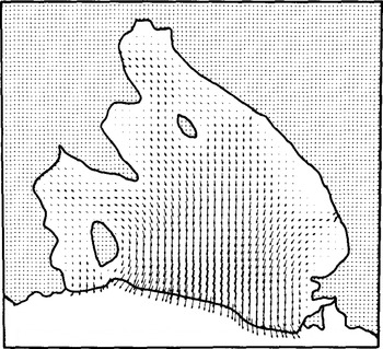
Fig.3. Flow vectors from run 2. Magnitudes are given in Figure 4.

Fig.4. Ice-velocity contours from run 2 in units of m a−1.

Fig.5. Vertical strain-rate contours from run 2 in units of 10−10 s−1 (negative for ice-shelf thinning).
Aside from the obvious error introduced by these technical problems, model sensitivity to several other effects can be addressed. Run 2 had qualitatively better results than run 1, because the variable B tended to stiffen (soften) the ice where the simulated flow was too high (low). We anticipate that the cross ice-shelf variations of B that ultimately yield the best fit between model and data can be inverted to give us valuable information regarding the temperature depth profile and basal-melting rates. Another discrepancy between model and observation is that the model does not maintain the high speeds and consolidation of the ice-stream injecta. Possibly this is because the ice streams themselves cannot be adequately resolved by the 22 km grid scale; the model retained correct volume flux by representing the ice streams as wider and slower moving than in reality. Afiner grid will overcome this problem. Finally, crevassing, rifting, and development of preferred ice fabric are important physics that are not incorporated by the model at this time.
Run 3 is distinct from runs 1 and 2 because we placed a hypothetical ice rise down-stream of the Crary Ice Rise at a location known as M12. The results are shown in Figures 6 and 7. The effect is (i) to reduce the ice velocity up-stream of M12, and (ii) to alter the vertical strain-rate field. Apparent in the simulated vertical strain-rate fields around Crary Ice Rise and M12 is a distinctive icer i se signature. Horizonal flow convergence occurs up-stream of the ice rise, and horizontal flow divergence occurs down-stream of the ice rise. This signature can be attributed to the compressive stresses associated with the back pressure exerted on upstream ice by the ice rise, and by the state of tension in the lee of the ice rise as ice is dragged away by faster-moving ice on either side. In run 3, the down-stream portion of the signature of Crary Ice Rise is almost cancelled by the up-stream portion of the signature of M12. This is also seen in the field data (Thomas and others in press): down-stream of Crary Ice Rise, there is no evidence of strong horizontal ice divergence, yet near the hypothetical M12 ice rise, there is the distinctive flow convergence suggestive of the up-stream portion of an icer i se signature. Debris-laden ice may be responsible for internal echoes in the radio echo-sounding prof iles near M12 (Jezek personal communication). However, there are no records of an ice rise in this area; if it exists, it does not appear to be associated with any surface crevassing or a rise in surface elevation. Perhaps the ice in this region is sliding over shoaling sea bed to form ice rumples, with little reduction in ice velocity, but encountering sufficient resistance to affect nearby strain-rates.

Fig.6 Ice-velocity contours from run 3 with hypothetical ice rise in units of m a−1.

Fig.7 Vertical strain-rate contours from run 3 with hypothetical ice rise in units of 10−10s−1 (negative for ice-shelf thinning).
We believe that the ice-rise signature and the modification of this signature by coordination of icerise locations is avital dynamic process. If, for instance, there are no ice rumples near M12, horizontal divergence down-stream and strong horizontal convergence up-stream of Crary Ice Rise will tend to cause the grounding-line perimeter of the ice rise to migrate up-stream along a sea-bed ridge by the process of up-stream grounding and down-stream ungrounding. The position of the Crary Ice Rise perimeter would thus retrograde with respect to the bulk ice movement. The existence of ice rumples downstream of Crary Ice Rise could prevent the retrograde motion by reducing ice divergence in the lee of the ice rise. We suggest that the apparently long-term historical presence of Crary Ice Rise (deduced from its dome elevation (Reference MacAyeal and ThomasMacAyeal and Thomas 1980)) is attributable to transient ice-rumple formation and decay near M12. These transient ice rumples may undergo retrograde displacement along the sea-bed ridges over which they form, so that an ice rise is never able to form. Despite their transience, repeated ice-rumple formation throughout the recent past may have prevented the retrograde displacement of the down-stream edge of Crary Ice Rise. The up-stream edge of Crary Ice Rise may be undergoing retrograde translation anyway, as suggested by Thomas and Reference Bentley, Clough, Jezek and ShabtaieBentley (1978). We recommend that the interaction between transient ice rises on the Ross Ice Shelf be studied further as a possibly important dynamic process.
Conclusion
Ice-shelf spreading is driven by the tendency of the less dense ice to override the more dense seawater, thereby allowing the ice/sea-water system to achieve minimum potential energy. Our finite element model reproduces this process by performing a detailed numerical account of the ice-shelf energy budget. The present model simulations have yielded encouraging results, and suggest that continued model improvement will result in a reliable scientific tool useful for reproducing field observations and for examining past and future ice-shelf scenarios. Moreover, the model can be used to investigate ice-shelf processes, such as transient ice-rise interaction, that cannot be fully illuminated by costly and lengthy field programs alone.
To improve the model's performance and provide close agreement with observations, we intend to: (i)obtain rapid convergence of viscosity to satisfy Glen's flow law, (ii)account for sub-grid scale stress variability such as rifting and thermal/fabric induced shear banding, (iii)improve the compatibi lity between ice - rise location, ice-stream inflow, and other influential features with the ice-thickness pattern used as model input (excessive variability in the simulated strain-rate patterns may result largely from grid interpolation errors while compiling the locations of ice rises and the observed ice-thickness patterns around them), (iv)explore the use of stressspecified instead of velocity-specified boundary conditions at the sides of and beneath grounded areas of ice shelf and alongside mountain walls, (v)find parameters for sub-grid scale ice-shelf grounding and ice-rumple formation, and (vi)improve our treatment of ice-shelf temperature variations in regions of high strain-rate.
Acknowledgements
We thank W F Schmidt, W Gray, F A Dahlen, R Bindschadler, K Bryan, J Sarmiento, I Held, M Jackson, T Pepin, J Zwally, and P Tunison for useful discussions and help in the preparation of this paper. D R MacAyeal was supported in part by ARL/NOAA grant NA80 RA00156, by the Geophysical Fluid Dynamics Program of Princeton University, and by Applied Research Co.


