


INTRODUCTION
Ice dynamics can play a significant role in glacier change and can confound the attribution of observed glacier changes to climate, particularly in regions characterized by high concentrations of surge-type or tidewater glaciers (e.g. Arendt and others, Reference Arendt2008; Larsen and others, Reference Larsen2015). Understanding ice dynamics, including its unstable manifestations, has therefore both inherent and applied appeal. Surge-type glaciers undergo episodic flow variations, in which the fast phase is usually associated with disruption of the subglacial drainage system (see Cuffey and Paterson, Reference Cuffey and Paterson2010; references therein) and may require a thermal transition at the bed (e.g. Robin, Reference Robin1955; Clarke, Reference Clarke1976; Murray and others, Reference Murray, Strozzi, Luckman, Jiskoot and Christakos2003). For glaciers that surge in the style of the well-studied Variegated Glacier (e.g. Kamb and others, Reference Kamb1985; Murray and others, Reference Murray, Strozzi, Luckman, Jiskoot and Christakos2003), the fast phase may begin in winter and persist for one or two summers, implying that the surge precludes the development of an efficient summer drainage system (e.g. Nienow and others, Reference Nienow, Sharp and Willis1998). While a vigorous surge may suspend the ordinary seasonal cycle, meteorological conditions can influence the progression of a surge or even lead to its termination (e.g. Eisen and others, Reference Eisen, Harrison and Raymond2001; Harrison and others, Reference Harrison2008).
The seasonal cycle of basal hydrology and dynamics that characterizes many alpine glaciers (e.g. Mair and others, Reference Mair, Nienow, Sharp, Wohlleben and Willis2002) bears some resemblance to the hydrologically driven surge cycle (e.g. Fowler, Reference Fowler1987; Kamb, Reference Kamb1987), albeit operational on much shorter timescales. In both cases, inhibition of the basal drainage system combined with an abundance of water leads to glacier acceleration, until an efficient drainage system can evacuate the stored water. While the classical interpretation of temperate glacier surges defines a clear separation between quiescence and surging (Kamb, Reference Kamb1987), recent work has suggested the possibility of a more progressive transition (Frappé and Clarke, Reference Frappé and Clarke2007; Sund and others, Reference Sund, Eiken, Hagen and Kääb2009) even for temperate glaciers (Jay-Allemand and others, Reference Jay-Allemand, Gillet-Chaulet, Gagliardini and Nodet2011). The identification of several ‘slowly surging’ glaciers (e.g. Frappé and Clarke, Reference Frappé and Clarke2007; De Paoli and Flowers, Reference De Paoli and Flowers2009), which have a history of surging in the classical sense but exhibit elevated flow speeds over years to decades, raises the question as to how these surge cycles interact with seasonal cycles and to what extent they influence one another.
Here we focus on short-term velocity variations of a slowly surging glacier, with the aim of understanding the intersection of long-term dynamic evolution and short-term meteorological response. We use static and kinematic GPS measurements made over two summers at three locations, along with annual stake velocities and modelled melt rates, to examine sub-seasonal velocity variations in the vicinity of the surge. We then use an idealized model of dashpots and frictional elements to explore longitudinal coupling in the region of interest.
Study area
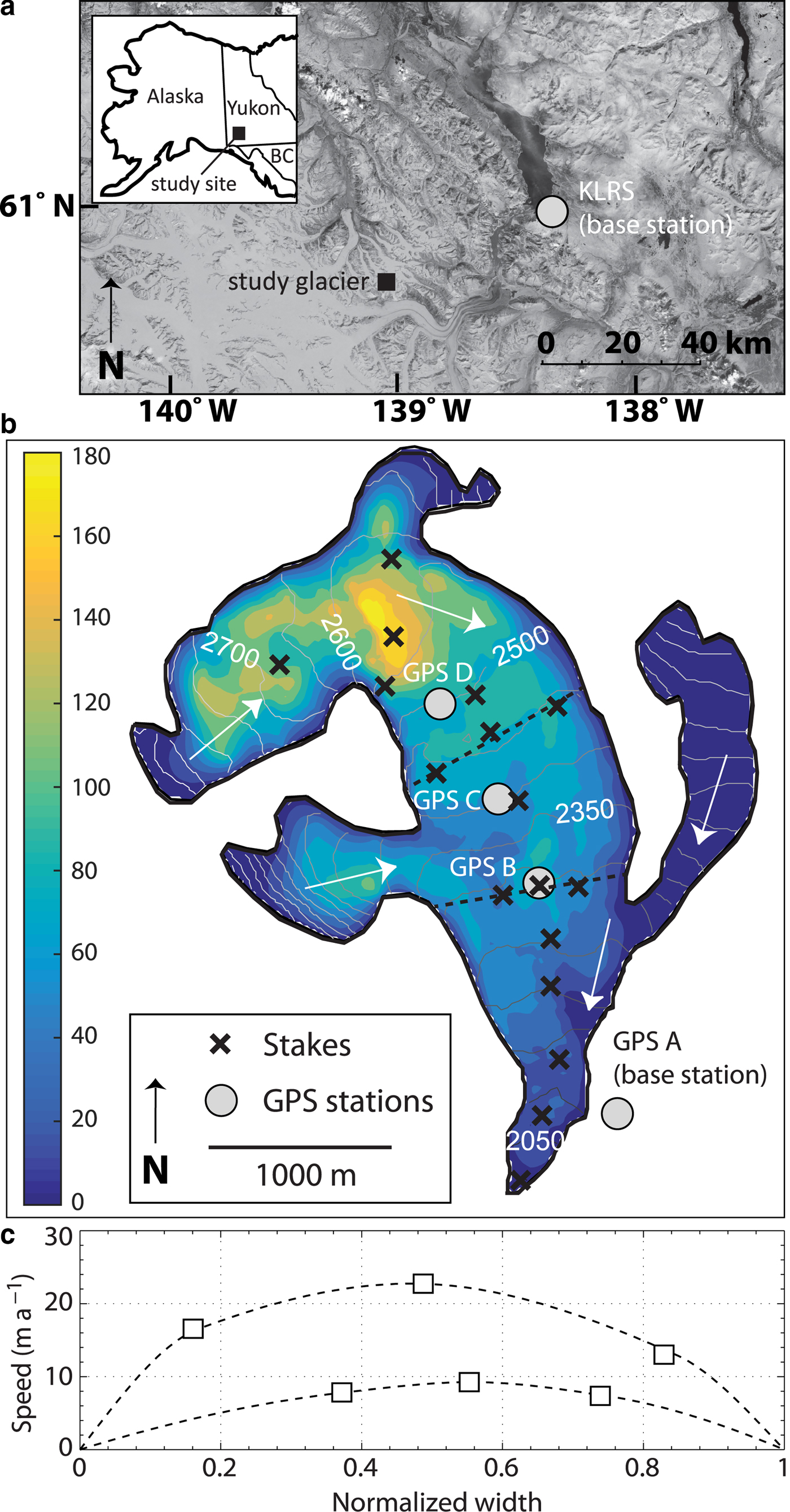
The study site is situated on the continental (lee) side of the St. Elias Mountains of southwest Yukon, Canada (Fig. 1). This region is characterized by extensive ice cover (e.g. Berthier and others, Reference Berthier, Schiefer, Clarke, Menounos and Rémy2010), by an abundance of surge-type glaciers (e.g. Clarke and Holdsworth, Reference Clarke and Holdsworth2002) and as having among the highest rates of glacier mass-loss worldwide (e.g. Gardner and others, Reference Gardner2013). The particular glacier of interest here was originally targeted as part of a study to understand regional variability of glacier response to climate (e.g. MacDougall and Flowers, Reference MacDougall and Flowers2011). It is 5.3 km2 in area, ranges in elevation from 1970 to 2960 m a.s.l. and has mean and maximum ice thicknesses of 64 m and 200 m, respectively (Wilson, Reference Wilson2012). Ice-penetrating radar and direct measurements of englacial temperature have revealed a polythermal structure, with a temperate accumulation area and cold ice concentrated near the terminus (Wilson and others, Reference Wilson, Flowers and Mingo2013). The central region of the glacier, on which this study focuses, is characterized by temperate ice near the bed and cold ice near the surface. The thickness of the cold shell increases down-glacier until cold conditions penetrate the entire ice column, such that the glacier is likely cold bedded in some areas near the terminus (Wilson and others, Reference Wilson, Flowers and Mingo2014).

Fig. 1. Study area. (a) Location of study glacier in the St. Elias Mountains of southwest Yukon, Canada (inset). Regional GPS base station KLRS is also shown. Image provided through NASA's Scientific Data Purchase Project and produced under NASA contract by Earth Satellite Corporation. (b) Study glacier detail. Surface topography is contoured in grey at intervals of 50 m a.s.l. with locations of stakes (crosses) and GPS stations (circles) marked. Ice thickness (m) is shown in colour with the scalebar to the left. Note that the eastern tributary was not surveyed and has since detached from the glacier. Dashed lines show transects from which transverse velocity profiles were constructed (c). Note position of local base station (GPS A) adjacent to the glacier margin. Ice flow directions are indicated by arrows within the glacier margin. (c) Measured annual surface flowspeeds (squares) averaged over 2006–2012 for stakes along transects oriented perpendicular to the primary direction of glacier flow (dashed lines in b). The higher speeds were measured along the upper transect, between GPS receivers C and D; the lower speeds were measured along a transect running through the GPS B site. Dashed lines in (c) show interpolated/extrapolated transverse profiles of mean annual flowspeed.
The study glacier has a history of surging (Johnson and Kasper, Reference Johnson and Kasper1992), with known surges in 1951 and 1986/87. Recent data and modelling suggest that a ‘slow surge’ as described by Frappé and Clarke (Reference Frappé and Clarke2007) is presently underway (De Paoli and Flowers, Reference De Paoli and Flowers2009; Flowers and others, Reference Flowers, Roux, Pimentel and Schoof2011). The region exhibiting elevated flow speeds is limited, but lies below the current ELA at ~2550 m a.s.l. The surge-front occurs at an approximate elevation of 2300 m a.s.l. (just above GPS B in Fig. 1) and is marked by a transition from anomalously high sliding speeds above, to nearly stagnant ice below (Flowers and others, Reference Flowers, Roux, Pimentel and Schoof2011).
DATA AND METHODS
GPS data
Three Trimble® R7 receivers with Zephyr™ geodetic antennas were deployed for various intervals during the summers of 2007 and 2008 (see Table 1). Antennas were mounted on threaded steel poles drilled several metres into the ice. Receivers were mounted in waterproof enclosures attached to the poles, while batteries were stored in dry bags that moved down with the ablating glacier surface. Two 30 W solar panels were mounted on separate structures at each station so as to minimize the wind disturbance to the GPS antenna mounts.
Table 1. Temporal coverage of GPS data used in this study. DOY, Day of Year. On-ice receivers (GPS B, C, D) were deployed for 31–35 d from late July to late August 2007 and 58–60 d from mid-July to mid-September 2008. GPS D is omitted in 2007 due to a power failure causing most data to be lost. Where the record lengths otherwise differ from the deployment dates, data were omitted due to poor quality. GPS A and KLRS are temporary local and regional base stations, respectively (see Fig. 1)

Preliminary GPS work in 2006 identified anomalously high flow speeds in the central ablation area, later interpreted as the slow surge. In 2007 and 2008 the receivers better sampled this region, with GPS D positioned toward the upper end of the surging region, GPS C within the surging region and GPS B just below the surge front (Figs 1, 2). All three receivers were deployed on structures that remained in the ice from 2007 to 2008. A power failure led to loss of all but 8 d of data from GPS D in 2007. Data from this receiver are therefore excluded from the 2007 analysis.

Fig. 2. Centreline velocity structure of study glacier. (a) Locations of GPS receivers B, C, D with modelled flowband speeds (colour) and glacier surface and bed topography (left axis). Flowband model is tuned to match measured annual surface velocities at stake locations (not shown) (see Flowers and others, Reference Flowers, Roux, Pimentel and Schoof2011). Annual (black line) and summer (grey line) surface flowspeeds simulated with tuned model (right axis). Dotted line shows simulated surface speeds without the enhanced sliding required to match stake data. (b) Difference between stake velocities measured over 1–3 weeks in summer (July–early August) and those measured annually, 2006–2012. Note that GPS receivers C and D are situated in a zone of enhanced sliding and pronounced seasonal acceleration, with the maximum difference between summer and annual speeds occurring at C.
Receivers were programmed to log with a sampling interval of 15 s in 2007 and 2 s in 2008. A temporary local base station within 2 km of the receivers (GPS A; Fig. 1) logged data at 15 s intervals in 2007. A temporary regional base station, logging at 2 s intervals, was established by the University of British Columbia in 2008 at a distance of 45 km from the study site (‘KLRS’; Fig. 1). We process the GPS data to daily static positions using the MIT-GAMIT/GLOBK software package (Herring and others, Reference Herring, King and McClusky2006). In addition to our own local and regional base stations, we make use of International GNSS (global navigation satellite systems) Service (IGS) reference stations BEA2, AB44, AB48 and WHIT in 2006, and AB43, AB44 and WHIT in 2007/08. The baselines between the local IGS stations and the study area range from ~200 km for BEA2 and WHIT to ~575 km for AB48; IGS station data were not available with sufficient uniformity to justify weighting stations by their baselines.
The processed daily static positions were compared with sub-daily solutions processed with a moving-baseline approach (RTKLIB: Takasu (Reference Takasu2009)), which yields precise relative positions between moving receivers. Details of the moving-baseline method can be found in the RTKLIB Manual (v2.4.2 http://www.rtklib.com/prog/manual_2.4.2.pdf). Comparison of relative receiver positions derived from the daily static solutions in 2008 with the moving-baseline results showed very good agreement and give us confidence that the daily static solutions adequately describe the glacier motion (e.g. King, Reference King2004). Due to the combination of satellite geometry, receiver positions in a steep-walled valley and the long baseline from the KLRS site in 2008, kinematic solutions at sub-daily timescales were deemed unreliable, thus we restrict our analysis to daily solutions.
In addition to position uncertainties associated with the processing, there are significant errors associated with progressive tilting of the mounting structure for GPS C in both 2007 and 2008. Due to a combination of initial installation depth and local meltrates, the pole on which GPS C was mounted was the highest of the three at the end of both melt seasons. Using pole height measurements and photographs taken when the station was dismantled, we estimate the vertical and horizontal contributions of this tilt to the total displacement of the station. In 2007 GPS C tilted a total of 8° over a maximum of 31 d, producing horizontal and vertical antenna displacements of 0.39 and 0.03 m, respectively. These displacements contribute to the total measured horizontal and vertical displacements of 3.06 and 0.40 m, respectively, but do not reflect glacier motion. In 2008 the tilt reached 21° over a maximum of 58 d, contributing 0.87 and 0.16 m to the total measured horizontal and vertical displacements of 5.10 and 1.13 m, respectively. The apparent motion due to tilt was detected in both the static daily and moving-baseline processing methods. In both years, the direction of tilt is close to the direction of motion.
We construct what we henceforth refer to as ‘corrected’ position records for GPS C by making assumptions about the temporal distribution of station tilt. We perform repeated calculations assuming tilt rate is (1) constant in time, (2) increasing linearly with time and (3) proportional to cumulative melt, calculated as described below. We present the results of correction 3, as the most physically motivated, and use the range of results of all three corrections to empirically estimate uncertainty on the GPS C records. Daily velocities are computed by applying a two-point centred difference to the cumulative horizontal displacement curve constructed from the corrected daily GPS solutions. Uncertainties estimated during the processing, including those associated with the tilt correction for GPS C, are propagated using standard error analysis (e.g. Taylor, Reference Taylor1997) in calculations of displacement and velocity.
Stake velocities
Repeated real-time kinematic (RTK) and post-processed kinematic (PPK) GPS surveys of 16–18 stakes from 2006 to 2012 provide point values of glacier surface displacement from which velocity can be calculated. Stake velocities provide a spatial and temporal context for the daily GPS results. The stake network spans elevations from the glacier terminus to the central accumulation zone (Fig. 1), and is also used in the melt modelling described below. Stake surveys are carried out with Trimble® GPS equipment identical to that described above, with GPS A serving as the base station. Annual velocities are measured between July of each year (2006–2012), while short-term ‘summer’ velocities are measured during 1–3 week periods in July or early August. Although we refer to these as ‘summer’ stake velocities, they represent brief periods during the summer season, rather than velocities representative of the entire melt season. These velocities probably under-estimate the highest seasonal flow rates, as the ‘spring event’ is thought to occur earlier in the season at this site (Personal communication from C. G. Schoof).
GPS heights and dynamic thickening rates
Vertical motion of the GPS stations is the sum of the vertical strain rate, bed-parallel motion and the rate of ice/bed separation (e.g. Anderson and others, Reference Anderson2004; Bartholomaus and others, Reference Bartholomaus, Anderson and Anderson2011). We use a 30 m DEM of the glacier bed obtained from extensive radar sounding (Wilson and others, Reference Wilson, Flowers and Mingo2013) to determine bed slopes in the two coordinate directions of ice motion (Easting, Northing) in the vicinity of each GPS station. Local bed slopes are computed separately for 2007 and 2008 to account for station displacement relative to the bed between years. The map-view orientation of GPS motion is used to appropriately assign height changes due to motion in the two coordinate directions, where bed slopes may differ. Surface height changes due to bed-parallel motion are then subtracted from the GPS height record.
Uncertainty in bed slopes contributes to uncertainty in the estimated bed-parallel component of vertical motion. Bed-slope uncertainty arises from numerous sources, including radar-system and GPS hardware, data processing, survey timing and ice-thickness interpolation scheme (see Wilson, Reference Wilson2012, for details). Empirically, we find that interpolated ice depths and borehole lengths differ by an average of ~6% (Wilson and others, Reference Wilson, Flowers and Mingo2013). Considering that bed slopes are computed based on differences in adjacent surface slopes and ice depths, we assign a value of 15% to represent the uncertainty in the estimated bed-parallel component of motion. This uncertainty is propagated along with the uncertainty on the processed GPS heights to obtain an uncertainty on the relative height corrected for bed-parallel motion. Uncertainties in GPS height relative to height changes, combined with uncertainties in the estimated vertical strain rates, are sufficiently large that meaningful estimates of bed separation cannot be obtained from our data.
To estimate the mean rates of dynamic thickening in the region between GPS B and D, we calculate volume fluxes in and out of the region and simply divide the change in volume by the enclosed surface area. This calculation is performed separately for subregions B–C, C–D and B–D, and requires estimates of depth-averaged velocity across the width of the glacier at the three flux gates, which intersect each of the GPS stations. We estimate the flux contributions of deformation and sliding separately. Using the flowband modelling results of Flowers and others (Reference Flowers, Roux, Pimentel and Schoof2011), we estimate a constant rate of ice deformation at each station and assume motion in excess of this value can be attributed to sliding. Though deformation rates have been documented elsewhere to vary on short timescales, summer flow variability is expected to be dominated by sliding (e.g. Ryser and others, Reference Ryser2014). We estimate the spatial variation of the deformation rate using the shallow-ice approximation and an assumption of constant surface slope. Under these assumptions, the surface speed due to deformation at any point y along the flux gate scales as (h y/h GPS) n+1 where h y and h GPS are the ice thicknesses at the point of interest and at the relevant GPS station, respectively, and n = 3 is Glen's exponent. Vertically integrating the theoretical deformation rate profile then allows us to estimate the temporally constant but spatially variable contribution of the deformation rate to the flux across any of the flux gates.
We use the GPS records themselves, with the local contribution of the deformation rate subtracted, to represent the temporal structure of sliding variation across the flux gates. The spatial variation of this sliding contribution requires that we scale the GPS sliding records to obtain appropriate sliding magnitudes across the gates. To do this, we make use of mean annual surface speeds measured at stakes that form transects roughly orthogonal to the glacier centreline (see dashed lines in Fig. 1b). We fit curves to the measured speeds, assuming speeds vanish at the glacier margin, to construct characteristic shapes for the surface-speed profiles across the transects (Fig. 1c). We then scale the two fitted profiles (one for GPS B, the other for GPS C and D) using the mean annual surface speeds measured at the GPS stations, accounting for the fact that the stations are not necessarily positioned at the fastest point along the profile. The curve used for GPS B is derived from measurements transverse to this station, while the one used for GPS C and D is derived from measurements across a transect between these two stations (dashed lines, Fig. 1b). The result is a dimensional transverse profile of mean annual surface speed at each of the three flux gates. By subtracting the dimensional transverse profiles of surface speed due to deformation, we are left with dimensional transverse profiles of surface speed due to sliding. These are normalized by dividing by the mean annual sliding speed at the GPS locations to obtain a transverse profile of relative sliding magnitude that can be used to extrapolate the time-dependent sliding speed from the GPS locations across the flux gates. Each of the three flux gates is discretized into 200 equally spaced intervals across the glacier surface. The sliding speeds and the depth-averaged speeds due to the deformation rate, obtained as described above, are summed and then multiplied by the local ice thickness and the width of the discretization interval to obtain the volumetric flux at each (daily) time step.
Our approach to estimating dynamic thickening allows for both spatially and temporally variable ratios of surface- to depth-averaged flowspeed, though it does not account for temporal variations in deformation rate. It is predicated on the validity of assuming transverse profiles of mean annual surface speed, derived from sparse stake measurements, adequately represent the transverse structure of surface speed across the flux gates. We have done several tests to examine the sensitivity of results to different approaches, including (1) using the transect at GPS B, rather than the higher transect, to represent the surface flowspeed structure at GPS C, (2) interpolating/extrapolating summer flowspeeds, rather than mean annual flowspeeds, to represent the surface flowspeed structure across the transects and (3) relaxing the constraint of zero speed at the glacier margin in the above extrapolations. We have also experimented with alternative ways of extrapolating the GPS records across the flux gates, including a simple method that assumes spatially uniform ratios of surface- to depth-averaged flowspeed. In all cases, we find that time-averaged dynamic thickening rates differ by <12% relative to our reference model.
Surface melt
We simulate hourly melt rates across a 30 m glacier surface DEM using the temperature-index model of Hock (Reference Hock1999), which modifies the degree-day factors with a term that depends on potential direct solar radiation. The model is forced by air temperatures measured with a shielded HMP45C212 TRH probe installed at a nominal height of 2 m above the glacier surface at an automatic weather station (AWS) near GPS B. We extrapolate temperature with a locally measured lapse rate of −6.4 K km−1 (unpublished data, Simon Fraser University). Cumulative ablation at the stake locations is used to calibrate the model parameters individually for each year (see MacDougall and Flowers, Reference MacDougall and Flowers2011; Wheler and others, Reference Wheler2014, for details). Though model parameters can vary substantially from year-to-year, this tuning procedure yields more accurate estimates of melt than one that adopts a single set of parameters calibrated across all years. Modelled melt has a similar temporal structure at all locations, because it is based on a single measured temperature record. Melt amounts differ by location due to the applied temperature lapse rate and the dependence of the degree-day factor on potential direct solar radiation and surface type (snow versus ice). Surface type is an output of the model, based in part on snow depths and densities measured in May, July and September of each year, and a measured time series of snowfall during the melt season (see Wheler and others, Reference Wheler2014, for details).
Mechanical model
To explore glacier dynamics in the region of interest, between GPS B and GPS D in Figures 1, 2, we construct a simple model using translational dampers (dashpots) and friction elements in the Matlab Simscape™ environment (Fig. 3). Such mechanical models, usually comprising interconnected springs and dashpots, are a common means of representing the fundamental behaviour of viscoelastic materials. They have been used in glaciology to model sea ice (e.g. Hopkins and others, Reference Hopkins, Hibler and Flato1991) and to understand the stick/slip behaviour of ice streams (e.g. Bindschadler and others, Reference Bindschadler, Vornberger, King and Padman2003; Sergienko and others, Reference Sergienko, MacAyeal and Bindschadler2009; Winberry and others, Reference Winberry, Anandakrishnan, Alley, Bindschadler and King2009; Goldberg and others, Reference Goldberg, Schoof and Sergienko2014).

Fig. 3. Matlab Simscape™ model with 7 blocks, each of which represents a ~0.6 km-long section of the glacier. All blocks are configured as Type I or Type II (lower right), with Type I comprising a single dashpot per block and Type II a combination of three dashpots with a single translational friction element. The model is driven by a prescribed speed imposed at one of three nodes corresponding to the positions of GPS B, C or D, and the responses measured at the other two station locations. Configuration shown has the forcing applied at GPS C and response measured at B and D. In the interest of reproducibility, all model components have been included and are labelled as in the Matlab Simscape™ environment. ‘Simulink–PS’ and ‘PS–Simulink’ converters convert unitless Simulink signals to physical signals (PS) and vice versa. ‘Ideal translational velocity source’ applies the forcing in the ‘Signal builder’ as a velocity at the point of attachment (here GPS C). Signals ‘uB’, ‘uC’ and ‘uD’ represent the time series of measured speed at each GPS station. ‘Ideal translational motion sensors’ detect the system response at the points of attachment (here GPS B and D) and provide output to the ‘Scopes’ through the ‘PS–Simulink converters’. The ‘Solver Configuration’ block contains numerical parameters and settings such as time step and convergence criterion.
Our model comprises 7 blocks connected in series, with each block representing a ~0.6 km-long section of the glacier. The series of blocks is situated between two ‘mechanical translational references’ (Fig. 3), which represent the glacier headwall and terminus, and impose zero-displacement boundary conditions at either end of the model domain. We consider two different block configurations: a single dashpot per block, which crudely represents the effective viscosity of the glacier (Type I), or a combination of dashpots with a translational friction element (Type II) intended to more explicitly represent ice deformation and sliding (Fig. 3; lower right). The translational friction element must be connected in parallel (not series) with at least one dashpot to permit deformation in the absence of sliding, while the dashpots on either side of the friction element are required to permit forcing from either side of the block. The coupling of translational friction with viscous elements in this way acknowledges that sliding must ultimately be accommodated by deformation (e.g. lateral shearing, longitudinal stretching or compression). We omit springs from the model, as the daily resolution of our GPS data is unlikely to reveal elastic behaviour.
Translational friction elements in Matlab Simscape™ assume Stribeck–Coulomb–viscous behaviour, with the sum of the Stribeck and Coulomb friction equal to the static friction. In our application, we set the Stribeck and viscous friction to zero, the Coulomb friction to a reference value of 109 Pa and the dashpot damping coefficient to
 ${10^{16}}\;{\rm N}\;{\rm s}{\kern 1pt} {{\rm m}^{ - 1}}$
. We estimate the reference value of the damping coefficient based on the characteristic viscosity of ice, and the Coulomb friction based on an assumed basal shear stress of 1 bar and sliding speeds inferred for our study area (De Paoli and Flowers, Reference De Paoli and Flowers2009). The precise values of the parameters are not of primary importance, as shown later.
${10^{16}}\;{\rm N}\;{\rm s}{\kern 1pt} {{\rm m}^{ - 1}}$
. We estimate the reference value of the damping coefficient based on the characteristic viscosity of ice, and the Coulomb friction based on an assumed basal shear stress of 1 bar and sliding speeds inferred for our study area (De Paoli and Flowers, Reference De Paoli and Flowers2009). The precise values of the parameters are not of primary importance, as shown later.
We drive the model with observed speeds at a given GPS location, and monitor the responses at the other two. These speeds are first corrected by subtracting an estimate of the local background speed (dotted line in Fig. 2), in an attempt to isolate motion due to seasonal variability, whether it be locally-forced or the result of longitudinal coupling. The numerical solver is configured to use the inbuilt ode23t. Model parameters are tuned by minimizing the RMSE between simulated and observed speed records at the GPS locations. Dashpot damping coefficients are varied over several orders of magnitude in increments of
 $1.0 \times {10^{16}}\;{\rm N}{\kern 1pt} {\rm s}\;{{\rm m}^{ - 1}}$
for the Type I model, while the Coulomb friction for the Type II model is varied over many orders of magnitude in order-of-magnitude increments. Dashpot damping coefficients are held fixed at the reference value for the Type II model, as we seek to isolate the explanatory power of variable bed friction in this case.
$1.0 \times {10^{16}}\;{\rm N}{\kern 1pt} {\rm s}\;{{\rm m}^{ - 1}}$
for the Type I model, while the Coulomb friction for the Type II model is varied over many orders of magnitude in order-of-magnitude increments. Dashpot damping coefficients are held fixed at the reference value for the Type II model, as we seek to isolate the explanatory power of variable bed friction in this case.
RESULTS AND DISCUSSION
Horizontal motion
Horizontal speeds calculated from daily GPS positions for 2007 and 2008 are shown in Figure 4. Uncertainties plotted for GPS C reflect the range of corrected records. Note that in 2008, the corrected speeds at GPS C are comparable with those at D for the first third of the record and then become much more variable. Toward the end of the record, speeds at GPS C decline well below speeds at D. The high variability of speeds at C after 2008 Day of Year (DOY) 215 is supported by all three tilt corrections (see grey shading in Fig. 4b), but we cannot rule out lower maximum and less variable speeds. If tilting occurred over only part of the record, or varied temporally in a manner not captured by one of the corrections, the true record of speed at GPS C would be different. We keep this caveat in mind in interpreting subsequent results.

Fig. 4. Horizontal speeds derived from daily displacements of GPS stations for (a) 2007 and (b) 2008, along with hourly and daily meltrates at AWS location (near GPS B) calculated with a temperature-index model (c, d). Shaded bands indicate propagated uncertainties. The uncorrected speed record for GPS C is shown as a dashed line (a) and (b) for comparison with the record corrected for tilting of the mounting structure. Horizontal lines in (a) and (b) show mean annual velocities at GPS B (green), GPS C (black), GPS D (blue). The melt model predicts that the glacier surface at GPS B was snow-free by 7 July 2007 (2007 DOY 188) and 19 June 2008 (2008 DOY 171), while GPS C is predicted to have been snow free by 18 July 2007 (2007 DOY 200) and 3 July 2008 (2008 DOY 185). The surface at GPS D remained snow-covered during the period of observation.
We calculate correlation coefficients, and cross-correlate time series, using standardized variables (mean subtracted, result normalized by standard deviation) to assess the basic relationship between daily melt and horizontal speed, and between the individual daily speed records (Table 2). We perform the cross correlations for lags ∈ [− 8, 8] days to preserve a minimum of 75% overlap between the time series being compared. Presentation of results is restricted to positive lags for the melt/speed cross correlations, as there is no plausible causative relationship between speed and melt (as modelled here) on the timescales in question. Our coarse GPS solutions prevent us from performing a more informative cross-correlation analysis to assess sub-daily leads and lags.
Table 2. Correlation coefficients between records of daily melt and daily speeds at GPS B, C and D (left column) and between speeds at the different stations (right column). Numbers in parentheses represent maximum values of cross correlations, along with lags at which these maxima occur. Where cross correlations peak at zero lag, values are identical to the correlation coefficients given

Speeds at GPS C correlate best with melt, with r = 0.35 in 2007 and r = 0.53 in 2008. Correlations between melt and speed are lower at GPS B and D, with r = 0.04 for GPS B in 2007, r = 0.47 for GPS B in 2008 and r = 0.28 for GPS D in 2008. Maximum cross correlation between melt and speeds at GPS B occurs at a lag of 3 d in 2007 (increasing r from 0.04 to 0.35), while cross correlation between melt and speeds at GPS D peaks at a lag of 2 d in 2008 (increasing r from 0.28 to 0.57). For GPS C, correlation with melt peaks at zero lag in 2007 and at a lag of 1 d in 2008. The positive lags above indicate melt leading speed.
The correlation coefficient between daily speeds at B and C is r BC = 0.34 in 2007 and r BC = 0.44 in 2008. In 2008 we also obtain r BD = 0.66 and r CD = 0.49, with r CD increasing to a maximum of 0.50 for a lag between D and C of 2 d. These statistics show that in both years, speeds at GPS B and D correlate with speeds at GPS C nearly as well as, or better than, they correlate with melt. This changes when lags are considered. The 2008 correlation of GPS D speeds with melt, at a lag of 2 d, exceeds the maximum correlation between speeds at GPS D and C. Though 2 d represents a significant lag for a melt response, we cannot rule out that GPS D may be responding to local melt. The 2007 correlation of GPS B speeds with melt, at a lag of 3 d, is comparable with the correlation between speeds at GPS B and C. If GPS B is responding to local melt, it is doing so with a lag greater than those of the upstream stations, including GPS D, which was situated in an area of continuous snow cover.
The above correlations characterize the relationships between records of flowspeed at a single lag, but careful examination of Figure 4b suggests there may be temporal variability in these relationships. Elevated speeds occur at all three stations in 2008 following two major melt episodes: one prior to 2008 DOY 200 and one from 2008 DOY 210–220. We observe that C leads B, and B leads D, in response to these melt events. Though our record does not capture the onset of the first event at GPS C in 2008, the declining speeds at C are suggestive of a peak response prior to 2008 DOY 196. Such a relationship is more difficult to pick out in 2007, though it appears that GPS C responds to the two periods of elevated melt (prior to 2007 DOY 219 and from 2007 DOY 224–234), while GPS B does not (with the possible exception of a prominent peak on 2007 DOY 233).
To identify temporal shifts in the relationships between stations, we compute running correlations of the speed records using a time window of 5 d (Fig. 5). Most periods of high correlation using the 5 d window are also apparent with arbitrary windows of 7 and 9 d. In 2007, two periods where r BC > 0.5 (and peaks above 0.8) occur between ~2007 DOY 220–226 and ~2007 DOY 234–236 (Fig. 5a). These intervals of high correlation are preceded by intervals of low or inverse correlation, themselves associated with elevated melt (red lines, Fig. 5a). We interpret the decorrelation as reflecting a more dynamic melt response of GPS C, relative to B. Though we cannot rule out a role for station tilt in this decorrelation, the alternating periods of correlation and decorrelation argue against tilt as the primary driver. We further note that the occurrence of the peak July flow anomaly in the vicinity of GPS C (Fig. 2b) is a robust feature derived from independent velocity-stake measurements over six melt seasons. The stake measurements indicate a peak in the July melt sensitivity near GPS C, consistent with the interpretation above.

Fig. 5. Running correlation coefficients r computed for records of horizontal speed at GPS B, C and D (left axes) shown with modelled hourly and daily meltrates at AWS location (red lines, right axes). Shading indicates r > 0.5. (a) GPS B and GPS C, 2007. (b) GPS B and GPS C, 2008. (c) GPS C and GPS D, 2008. (d) GPS B and GPS D, 2008.
Abrupt changes in station correlation occur in 2008 (Figs 5b–d). All records exhibit variable periods of high correlation during intervals of low melt, as in 2007 (e.g. just prior to 2008 DOY 211 and just after 2008 DOY 220 and 2008 DOY 234). GPS C again decorrelates with its neighbours, here after the peak of the largest melt event (2008 DOY 216 in Fig. 5b, 2008 DOY 215 in Fig. 5c). The dip in r BD around 2008 DOY 217 (Fig. 5d) is due to the prolonged response of GPS D to the 2008 DOY 210–220 melt event (see Fig. 4b for detail). The conspicuous plunge in correlation of all stations beginning on or after 2008 DOY 201, when melt is at a minimum, appears to conflict with the explanations given above. Upon inspection of Figure 4b however, this decorrelation can be explained as part of the lingering response to the first major melt event prior to 2008 DOY 200, which our GPS data only partially capture. Correlations between 2008 DOY 226–232 present an interesting picture, with r CD > 0.5 and r BC and r BD < 0.5. This is a period of relatively low melt at GPS B (red lines in Fig. 5), and even less melt at C and D (not shown). Most of the correlations in Figure 5 decline toward the end of the record as surface melt diminishes. We speculate that the ongoing velocity variability (Fig. 4) may derive from variable basal water pressures that occur in the absence of surface melt and that have been documented at this site (Schoof and others, Reference Schoof, Rada, Wilson, Flowers and Haseloff2014). Variable basal water pressures arising from episodic storage and release of englacial/subglacial water (e.g. Kingslake, Reference Kingslake2015) could explain velocity variability that is not clearly paced by surface melt, and therefore displays increased spatial heterogeneity.
Vertical motion
A consistent spatial pattern emerges in relative GPS heights: GPS B shows a nearly steady and monotonic increase in height in both years (Figs 6a, 7a), while GPS C exhibits an increase followed by a decrease in each year (Figs 6b, 7b). The height of GPS D increases almost monotonically in 2008, with most of the increase occurring in the first half of the record (Fig. 7c). Mean dynamic thickening rates computed for the region are generally positive in both years (Figs 6c, 7d), though episodic thinning may occur between GPS C and D (Fig. 7d).

Fig. 6. Relative height changes and estimated mean thickening rate for region B–C in 2007. (a) Relative height corrected for bed parallel motion (white line) derived from 2007 daily positions of GPS B. Shaded bands indicate uncertainties propagated from the original position solutions and the estimated uncertainty associated with removing the contribution of bed-parallel motion. Horizontal speed from Figure 4a (solid black line) and the raw relative height record including bed-parallel motion (dashed line) are shown for reference. Uncertainties are omitted to avoid clutter. (b) As in (a) but for GPS C. Raw relative height (dashed line) is truncated in the figure but reaches a minimum of −0.37 m. (c) Mean dynamic thickening rate calculated for region B–C. See text for details. Uncertainties shown do not include those due to alternative tilt corrections for GPS C.

Fig. 7. Relative height changes and estimated mean thickening rates in 2008. (a) Relative height corrected for bed parallel motion (white line) derived from 2008 daily positions of GPS B. Shaded bands indicate uncertainties propagated from the original position solutions and the estimated uncertainty associated with removing the contribution of bed-parallel motion. Horizontal speed from Figure 4b (solid black line) and the raw relative height record including bed-parallel motion (dashed line) are shown for reference. Uncertainties are omitted to avoid clutter. (b) As in (a) but for GPS C. Raw relative height (dashed line) is truncated in the figure but reaches a minimum of −0.95 m. (c) As in (a) and (b) but for GPS D. Raw relative height (dashed line) reaches a minimum of −0.59 m. (d) Mean dynamic thickening rate calculated for regions B–C, B–D and C–D. See text for details. Uncertainties shown do not include those due to alternative tilt corrections for GPS C.
Below we argue that the relative height records of GPS B, C and D reflect different combinations of the vertical strain rate, due to the generally compressive flow regime, and local ice/bed separation. The maximum relative height achieved by GPS C occurs in the neighbourhood of DOY 229 in 2007, and DOY 215 in 2008 (Figs 6b, 7b), in the middle of the last significant and sustained period of melt in the respective years (see Figs 4c, d). We further observe that during the rising limb of relative height for GPS C in 2007, prominent multiday peaks in horizontal speed occur coincident with accelerated rates of height increase (see peaks just after 2007 DOY 215, 220, 225 in Fig. 6b). This relationship between horizontal speed and vertical uplift is one of the hallmarks of ice/bed separation due to local cavitation, as described by Iken (Reference Iken1981) and Iken and others (Reference Iken, Röthlisberger, Flotron and Haeberli1983).
It is difficult to identify a similar relationship in 2008, where the magnitude of the relative height increase is smaller. Note that 2008 had less winter accumulation than 2007 (0.35 m w.e. versus 0.57 m w.e. glacier wide (Wheler and others, Reference Wheler2014)), while modelled cumulative ablation up to DOY 208 (beginning of 2007 GPS record) is similar for both years. Less accumulation would allow earlier access of surface meltwater to the bed in 2008, thus we might expect subglacial drainage system development to be more advanced (e.g. Nienow and others, Reference Nienow, Sharp and Willis1998; Anderson and others, Reference Anderson2004) for a given DOY in 2008 relative to 2007. Locally driven cavitation events may therefore be more difficult to observe in the portion of the 2008 melt season covered by our record.
Where extensional (positive) vertical strain rates occur, as suggested by regional dynamic thickening (Figs 6c, 7d), any decrease in relative height represents a decline in bed separation of equal or greater magnitude. By this logic, we can put a lower bound on the maximum ice/bed separation at GPS C based on the difference in relative height between the peak and the end-of-season value, where relative height appears to plateau: ~6 cm in 2007 and ~35 cm in 2008 with large uncertainties. We conclude that there is a component of ice/bed separation in the relative height records of GPS C, and thus a significant contribution of basal hydrology to the local dynamics.
In contrast, the relative height record of GPS B shows little to no evidence of local ice/bed separation in its steady and nearly monotonic increase through both the 2007 and 2008 records, well beyond the period of significant melt. The relatively smaller horizontal speed variations of GPS B make it difficult to detect any relationship between horizontal speed and relative height. However, a relationship between horizontal speed and relative height like that described for C can be identified in a brief record from GPS B in 2006 that covers an earlier part of the melt season. We surmise that the 2007 and 2008 relative height records of GPS B dominantly reflect local compression due to upstream flow conditions, at least during this phase of the melt season. Since all three receivers are located in the ablation area and are thus generally subject to longitudinal compressive strain rates, we should expect measured increases in relative height independent of any surge dynamics. A first-order estimate of the horizontal velocity profile in the absence of surging behaviour is given by the dotted line in Figure 2a. The difference in ice flux computed using the dotted versus solid velocity curves (not shown) suggests that the surge is the dominant driver of the vertical strain rate inferred at GPS B.
GPS D presents a more puzzling record of relative height (Fig. 7c), with an increase of ~30 cm over the first half of the 2008 record and a negligible change thereafter. Given that the contribution of bed-parallel motion has been removed, the remaining signal is the sum of the contribution from the vertical strain rate and bed separation. The contribution from one or both of these processes must change half way through the record in order to produce the change in slope in Figure 7c. If net dynamic thickening (positive strain rate) as indicated for Region C–D (Fig. 7d) is occurring at the location of GPS D, the relative height record of D (Fig. 7c) could be partially explained by increasing bed separation over the first half of the record and decreasing bed separation over the second half. An alternative explanation that does not require local ice/bed separation is that reduced ice influx from upstream sometime after 2008 DOY 220 shuts down dynamic thickening at GPS D. Due to the absence of GPS stations above D, we have no constraint on incoming ice flux (c.f. Fig. 7d).
The mean dynamic thickening rates in the region between GPS D and GPS B are positive in both years (Figs 6c, 7d), and twice as high in the lower region (between GPS B and C) compared with the upper (between GPS C and D). Thickening rates between GPS B and C averaged over the 2007 and 2008 records are 1.7 and 1.6 m a−1, respectively. These values are comparable with the annual net balance of ~−1.5 m a−1 measured in the vicinity of GPS B. For a glacier subject to a prolonged negative mass balance, local ablation rates should not be fully compensated by dynamic thickening. For a surging glacier, dynamic thickening should far exceed local ablation rates, such that a mass front propagates down-glacier. The study glacier exhibits intermediate characteristics, where the surge allows dynamic thickening rates higher than those expected for the mass-balance regime, but lower than those required to propagate a mass front.
Model results
To test the hypothesis that the surging region of the glacier drives some of the short-term dynamic variability above and below it, we force the model (Fig. 3) with observed speeds at one GPS station location and monitor the response at the other two (Fig. 8). The extent to which the modelled response matches the observed is suggestive of the relative role played by longitudinal coupling versus local forcing. Models driven by GPS B are not shown in Figure 8, as they fail to produce responses comparable with those measured at GPS C and D under any conditions. Note that all responses mimic the forcings in structure and phase. This is a consequence of the model being driven by an applied speed, and limits its explanatory power. The ‘mechanical translational references’ (Fig. 3) or hard stops at either end of the model, representing the headwall and terminus of the glacier, enforce a zero speed condition at these locations. The blocks that comprise the model therefore serve to partition the speeds between the node where the forcing is applied and the boundaries at either end.

Fig. 8. Matlab Simscape™ model results forced by 2008 flowspeeds at GPC (a, c, e) or GPS D (b, d, f) for Type I and II models (see Fig. 3). Untuned Type I model (left column) uses uniform damping coefficients for each model block, while tuned Type I model (middle column) allows damping coefficient to vary between blocks. Tuned Type II model (right column) uses uniform damping coefficients for all dashpots, but allows basal friction to vary.
The untuned Type I model results (Figs 8a, b) demonstrate that a simple model with spatially uniform glacier properties, represented by the dashpot damping coefficients, yields poor agreement between measured and modelled speeds. In the presence of uniform damping coefficients, the model response is fixed by glacier geometry as represented in the distribution of model blocks. Changing the value of the damping coefficient therefore has no effect on the results, unless spatial heterogeneity is introduced.
Better agreement between observed speeds and those simulated with the Type I model is achieved with spatially variable dashpot damping coefficients (Figs 8c, d), though the variation required to minimize RMSE between simulated and observed records differs when forcing the model at GPS C (Fig. 8c) versus at GPS D (Fig. 8d). The fit in Figure 8c is achieved by lowering the damping coefficient above GPS D (Blocks 1–3) to
 $0.7 \times {10^{16}}\;{\rm N}{\kern 1pt} {\rm s}\;{{\rm m}^{ - 1}}$
and increasing it below GPS B (Blocks 6–7) to
$0.7 \times {10^{16}}\;{\rm N}{\kern 1pt} {\rm s}\;{{\rm m}^{ - 1}}$
and increasing it below GPS B (Blocks 6–7) to
 $5 \times {10^{16}}\;{\rm N}\;{\rm s}{\kern 1pt} {{\rm m}^{ - 1}}$
from the reference value of
$5 \times {10^{16}}\;{\rm N}\;{\rm s}{\kern 1pt} {{\rm m}^{ - 1}}$
from the reference value of
 $1 \times {10^{16}}\;{\rm N}\;{\rm s}{\kern 1pt} {{\rm m}^{ - 1}}$
. Such a spatial pattern characterized by much higher viscosity below GPS B and slightly lower viscosity above GPS D, relative to the viscosity in region B–D, could be interpreted as consistent with the known thermal structure of the glacier: the accumulation area is temperate throughout the ice column, the ablation area below GPS B is predominantly cold and the zone between GPS B and D has a patchy structure dominated by warm ice near the bed (Wilson and others, Reference Wilson, Flowers and Mingo2013). It is worth bearing in mind that damping coefficients in the Type I model lump all resistance to motion, whether by deformation or sliding, into a single parameter.
$1 \times {10^{16}}\;{\rm N}\;{\rm s}{\kern 1pt} {{\rm m}^{ - 1}}$
. Such a spatial pattern characterized by much higher viscosity below GPS B and slightly lower viscosity above GPS D, relative to the viscosity in region B–D, could be interpreted as consistent with the known thermal structure of the glacier: the accumulation area is temperate throughout the ice column, the ablation area below GPS B is predominantly cold and the zone between GPS B and D has a patchy structure dominated by warm ice near the bed (Wilson and others, Reference Wilson, Flowers and Mingo2013). It is worth bearing in mind that damping coefficients in the Type I model lump all resistance to motion, whether by deformation or sliding, into a single parameter.
Results almost indistinguishable from those in Figure 8c can instead be obtained with dashpot damping coefficients of
 $1 \times {10^{16}}\;{\rm N}{\kern 1pt} {\rm s}\;{{\rm m}^{ - 1}}$
above GPS D (Blocks 1–3),
$1 \times {10^{16}}\;{\rm N}{\kern 1pt} {\rm s}\;{{\rm m}^{ - 1}}$
above GPS D (Blocks 1–3),
 $2 \times {10^{16}}\;{\rm N}{\kern 1pt} {\rm s}\;{{\rm m}^{ - 1}}$
between D and C (Block 4),
$2 \times {10^{16}}\;{\rm N}{\kern 1pt} {\rm s}\;{{\rm m}^{ - 1}}$
between D and C (Block 4),
 $1 \times {10^{16}}\;{\rm N}{\kern 1pt} {\rm s}\;{{\rm m}^{ - 1}}$
between C and B (Block 5) and
$1 \times {10^{16}}\;{\rm N}{\kern 1pt} {\rm s}\;{{\rm m}^{ - 1}}$
between C and B (Block 5) and
 $5 \times {10^{16}}\;{\rm N}\;{\rm s}{\kern 1pt} {{\rm m}^{ - 1}}$
below B. In this case, the coupling between C and D is increased to better transmit the forcing, rather than the coupling above D decreased to reduce the damping. In both cases, stiff ice is required below GPS B to attenuate the response.
$5 \times {10^{16}}\;{\rm N}\;{\rm s}{\kern 1pt} {{\rm m}^{ - 1}}$
below B. In this case, the coupling between C and D is increased to better transmit the forcing, rather than the coupling above D decreased to reduce the damping. In both cases, stiff ice is required below GPS B to attenuate the response.
When forcing the Type I model at GPS D, success is limited by the response at C. The tuned model results in Figure 8d are achieved with dashpot damping coefficients of
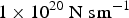 $1 \times {10^{20}}\;{\rm N}\;{\rm s}{\kern 1pt} {{\rm m}^{ - 1}}$
between D and C (Block 4),
$1 \times {10^{20}}\;{\rm N}\;{\rm s}{\kern 1pt} {{\rm m}^{ - 1}}$
between D and C (Block 4),
 $1 \times {10^{16}}\;{\rm N}{\kern 1pt} {\rm s}\;{{\rm m}^{ - 1}}$
between C and B (Block 5) and
$1 \times {10^{16}}\;{\rm N}{\kern 1pt} {\rm s}\;{{\rm m}^{ - 1}}$
between C and B (Block 5) and
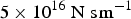 $5 \times {10^{16}}\;{\rm N}\;{\rm s}{\kern 1pt} {{\rm m}^{ - 1}}$
below B (Blocks 6–7). Tight coupling between D and C, represented by the orders-of-magnitude higher damping coefficient and hence viscosity of Block 4, is required to achieve the reported RMSE between simulated and observed speeds at C. The results do not depend on the damping coefficients of Blocks 1–3 when the forcing is applied at D.
$5 \times {10^{16}}\;{\rm N}\;{\rm s}{\kern 1pt} {{\rm m}^{ - 1}}$
below B (Blocks 6–7). Tight coupling between D and C, represented by the orders-of-magnitude higher damping coefficient and hence viscosity of Block 4, is required to achieve the reported RMSE between simulated and observed speeds at C. The results do not depend on the damping coefficients of Blocks 1–3 when the forcing is applied at D.
The more physically motivated Type II model (Figs 8e, f) does not perform objectively better than the tuned Type 1 model (Figs 8c, d), though we have arguably limited the model/data fit in choosing to vary only the value of the friction coefficient (rather than the dashpot damping coefficients as well) in the Type II model. When forcing the model at GPS D, the tuned Type I and Type II results are comparable at GPS B (RMSEs of 2.5 and 2.2 m a−1, respectively) and better than when forcing the model at GPS C (RMSEs of 3.4 and 3.5 m a−1, respectively). By contrast, the fit is particularly poor at GPS C when forcing the model at D (RMSE of 13.1 m a−1, Fig. 8f). Even this relatively poor fit requires frictionless conditions between GPD C and D, but is insensitive to the friction between GPS C and B over orders of magnitude. The requirement of a frictionless bed between GPS C and D in this case is consistent with the very tight coupling between these stations required in the tuned Type I model (Fig. 8d). When forcing the Type II model at GPS C instead, the best results are obtained by increasing basal friction below C and decreasing basal friction above. The results in Figure 8e employ friction values of 106 Pa above GPS D (Blocks 1–3), 105 Pa between D and C (Block 4), and 1011 Pa below C (Blocks 5–7). Such a pattern suggests the need to minimize sliding around and below B, and affirms the requirement for reduced basal friction between C and D. The range over which friction values must be varied to achieve this fit should not be over interpreted: the spectrum of behaviour between a frictionless bed and a no-sliding condition is set by the configuration of the dashpots in the model.
The similarity of results between tuned Type I and II models when forced by observed speeds at GPS C (Figs 8c, e), indicates that speeds at D and B can be equally well explained by spatial variations in bed friction only (Type II model) or spatial variations in the effective viscosity of the glacier (Type I). At face value, this outcome suggests that a very simple model of dashpots connected in series (Type I) performs as well as a more physically motivated model that attempts to separate deformation from sliding (Type II). However, the tuned Type II model suggests a pattern of bed friction roughly consistent with the current surge as well as the known glacier thermal structure. Though forcing the model at GPS D results in better model/data agreement at B than forcing the model at GPS C, D as a driver of variations at C is less compelling. Even when RMSE values are comparable between models forced at C and D, it is more difficult to justify the required parameters in the latter case. The model results, in combination with the results in Table 2, favour GPS C as the more likely driver.
SUMMARY AND OUTLOOK
We observe seasonal flow enhancement of a slowly surging glacier, with a maximum summer flow anomaly upstream of the surge front (GPS C). Horizontal and vertical motion analyzed from GPS records collected over two melt seasons suggest the region involved in the surge is most responsive to surface melt, and drives at least some of the short-term flow variability above (GPS D) and below (GPS B). Simple mechanical models of dashpots and frictional elements corroborate this possibility.
Horizontal speeds at GPS C correlate best with the melt record, while speeds at B and D correlate as well or better with speeds at C than they do with melt (Table 2, Fig. 5). Visual inspection and cross-correlation analysis of the speed records further suggest that GPS C leads B and D in the response to melt events (Figs 4a, b), which themselves give rise to decorrelation of GPS C from its neighbours. Velocities derived from independent stake measurements (Fig. 2b) show a peak in the July flow anomaly at C. GPS height records provide some evidence for ice/bed separation persisting deep into the melt season at C, but not occurring at B, supporting the notion of hydrologically forced sliding variability at C. Though the limited time period covered by our GPS data does not preclude a seasonal response of the glacier below the surge front (GPS B), the stake velocities (Fig. 2b) argue for the greatest seasonal sensitivity being in the vicinity of GPS C.
The sliding (and/or bed deformation) rates associated with the surge imply that elevated basal water pressures are widespread and sustained. We suspect this situation enhances the glacier's sensitivity to ordinary seasonal processes. High sliding rates would also inhibit the development of an efficient summer drainage system above the surge front, allowing prolonged seasonal sensitivity to meltwater input. A strain grid of 16 GPS stations deployed in the surging region of the glacier has now been established (see Flowers and others (Reference Flowers, Copland and Schoof2014) for a preview), with most receivers logging year-round. A complementary borehole drilling program to measure basal water pressures is also underway (Schoof and others, Reference Schoof, Rada, Wilson, Flowers and Haseloff2014). The spatial density of velocity data afforded by this GPS array, along with direct borehole observations of the basal drainage system, should provide answers to some of the questions posed here. Whether the surge is required to explain the observed seasonal sensitivity of the glacier remains an open question that could best be answered with data collected during other phases of the surge cycle.
ACKNOWLEDGEMENTS
Permission to conduct our field research was granted by the Kluane First Nation, Parks Canada and the Yukon Territorial Government, and would not have been possible without the field assistance of Chris Doughty, Brett Wheler, Jessica Logher and Andrew MacDougall in particular. We thank Eric Petersen for the meltrate calculations and the UBC glaciologists for feedback on the data processing and analysis. KLRS base station data were used with the permission of Christian Schoof, University of British Columbia. Logistical support from the Kluane Lake Research Station and Trans North Helicopters is greatly appreciated. We are grateful to the Natural Sciences and Engineering Research Council of Canada (NSERC), the Canada Foundation for Innovation (CFI), the Canada Research Chairs (CRC) Program, the Northern Scientific Training Program (NSTP) and Simon Fraser University (SFU) for funding. Tim Bartholomaus, one anonymous reviewer and Scientific Editor Matt Hoffman all provided thoughtful and constructive comments on the manuscript.


 Open access