


1. Introduction
For a single-component perfect gas, entropy perturbations are responsible for the so-called ‘excess density’ in Lighthill's acoustic analogy theory (Lighthill Reference Lighthill1952), denoting the difference between the overall density fluctuation and that associated with the acoustic perturbation. Entropy perturbations are thus the incompressible part of density perturbations. Physically, they can be generated by unsteady heat release, unsteady heat transfer or viscous effects. Entropy perturbations are silent when advected by uniform flows but generate sound when accelerated/decelerated (Marble & Candel Reference Marble and Candel1977). This generated sound is termed entropy noise and is an important contributor to indirect combustion noise (Ihme Reference Ihme2017; Tam et al. Reference Tam, Bake, Hultgren and Poinsot2019), which is highly relevant to thermoacoustic instabilities in gas turbines and rocket engines (Keller, Egli & Hellat Reference Keller, Egli and Hellat1985; Morgans & Duran Reference Morgans and Duran2016) and noise from aeroengines (Ffowcs Williams Reference Ffowcs Williams1977; Duran et al. Reference Duran, Moreau, Nicoud, Livebardon, Bouty and Poinsot2014).
For a quasi-1-D isentropic nozzle flow, the seminal theory of Marble & Candel (Reference Marble and Candel1977) predicts the sound generation using isentropic flow conservation equations across the nozzle for the zero-frequency limit. This was extended to any frequency by Duran & Moreau (Reference Duran and Moreau2013). In a recent laboratory-scale experiment for studying this (Rolland, De Domenico & Hochgreb Reference Rolland, De Domenico and Hochgreb2017), the flow was accelerated and then decelerated through a hole, comprising a sudden area contraction followed by a sudden expansion. The flow through the contraction remains largely attached and isentropic, while the sudden expansion causes a massive, non-isentropic flow separation. The aforementioned quasi-1-D isentropic theory was found insufficient for predicting the sound generation. To explain the difference, De Domenico, Rolland & Hochgreb (Reference De Domenico, Rolland and Hochgreb2019) proposed an empirical model which pointed to the flow non-isentropicity as the main mechanism responsible for it. However, the model was not designed to identify detailed sound sources and the explanation remains a hypothesis.
Even though the earliest theory of identifying entropy-related sound sources using an acoustic analogy was studied nearly 50 years ago (Morfey Reference Morfey1973; Ffowcs Williams & Howe Reference Ffowcs Williams and Howe1975), theoretical studies of this kind remain challenging. This is because the effects of mean flow non-uniformity on the acoustic propagation and entropy sound generation need to be properly distinguished, which becomes especially difficult in the presence of flow separation and vortex shedding. A more systematic derivation based on the stagnation enthalpy by Howe (Reference Howe1975) was used to study entropy noise for a nozzle with flow separation (Howe Reference Howe2010). However, quantitative validation is missing, and the key step of separating the stagnation enthalpy perturbation into acoustic and entropy components, in order to identify the entropy-related sound sources, needs to be clarified.
The key contributions of this paper are twofold. Firstly, we build on Howe's theory to derive a new form of the acoustic analogy, in which the acoustic and entropy perturbations are clearly distinguished. Secondly, we apply this new theory to the canonical case of a sudden area expansion, shown in figure 1, where the mean flow separation at the expansion edge generates a large recirculation zone. Sound is produced when an entropy wave applied at the inlet is decelerated by the flow. We use the theory to show that the presence and spatial extent of the recirculation zone is the main factor causing deviation from quasi-1-D, isentropic theory.
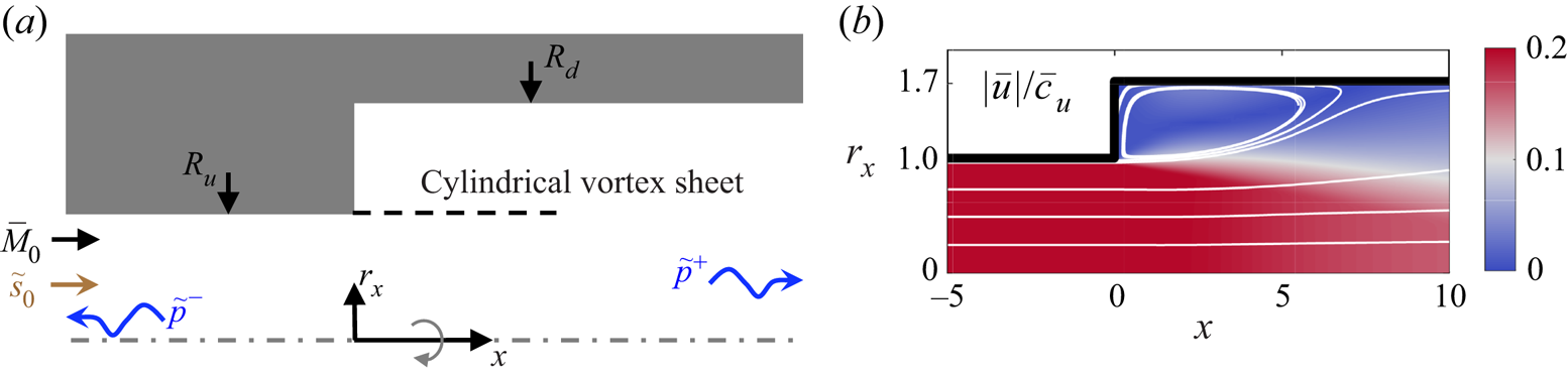
Figure 1. (a) A schematic view of an axisymmetric flow expansion with an incoming mean flow  $\bar {M}_0$ and entropy wave $\tilde {s}_0$ imposed at the inlet, and generated acoustic waves $\tilde {p}^{\pm }$. (b) Magnitude of the normalised mean velocity field. The white lines denote streamlines.
The theory is developed in § 2 and used to resolve the flow expansion problem in § 3 by using a Green's function method. Results are presented in § 4 and simplified models are proposed in § 5 to shed light on the physical mechanisms.
2. The acoustic governing equations
Neglecting mass sources, body forces and any heat addition and thermal diffusion, the conservation of mass, momentum and energy for a single-component thermally perfect gas gives
 \begin{gather} \frac{\partial \rho}{\partial t}+ \boldsymbol{\nabla}\boldsymbol{\cdot} (\rho \boldsymbol{u})=0, \end{gather}
 \begin{gather}\frac{\partial \boldsymbol{u}}{\partial t} +\boldsymbol{\nabla} B = \boldsymbol{u}\times \boldsymbol{\omega}+ T\boldsymbol{\nabla} s + \frac{1}{\rho} \boldsymbol{\nabla} \boldsymbol{\cdot} \boldsymbol{\tau}, \end{gather}
 \begin{gather}\rho T \frac{\textrm{D} s}{\textrm{D} t}= \boldsymbol{\tau} : \boldsymbol{\nabla} \boldsymbol{u}, \end{gather}
where  $\rho , t, \boldsymbol {u}, T$ and $s$ denote density, time, velocity, temperature and entropy, respectively, $B=h+|\boldsymbol {u}|^2/2$ is the stagnation enthalpy, $h$ the enthalpy, $\boldsymbol {\omega }=\boldsymbol {\nabla } \times \boldsymbol {u}$ the vorticity, $\boldsymbol {\tau }$ the viscous stress tensor, $\textrm {D} /\textrm {D} t = \partial / \partial t +\boldsymbol {u}\boldsymbol {\cdot } \boldsymbol {\nabla }$ the material derivative, and : the double dot product, such that ${\boldsymbol{\mathsf{M}}} :{\boldsymbol{\mathsf{N}}} ={tr}({\boldsymbol{\mathsf{M}}} {\boldsymbol{\mathsf{N}}}^\textrm {T})$. Dividing (2.1) by $\rho$ and taking $\partial /\partial t$, multiplying (2.2) by $\rho$ and taking the divergence, and then combining gives
 \begin{equation} - \rho \frac{\textrm{D}}{\textrm{D} t} \left( \frac{1}{\rho} \frac{\partial \rho}{\partial t}\right) + \boldsymbol{\nabla} \boldsymbol{\cdot}(\rho \boldsymbol{\nabla} B) = \boldsymbol{\nabla} \boldsymbol{\cdot} (\rho \boldsymbol{u}\times \boldsymbol{\omega}+ \rho T\boldsymbol{\nabla} s + \boldsymbol{\nabla} \boldsymbol{\cdot} \boldsymbol{\tau}). \end{equation}
Taking  $\boldsymbol {u} \boldsymbol {\cdot }$ (2.2), adding $(1/\rho )\partial p/\partial t$ to both sides, then using the relation $\textrm {d} B = \textrm {d}h + \textrm {d}|\boldsymbol {u}|^2/2$ and the generic thermodynamic relations $\textrm {d} h = \textrm {d} p/\rho + T \textrm {d} s$ and $\textrm {d} \rho = \textrm {d} p/c^2 - \rho \textrm {d} s/ c_p$ (where $c$ is the sound speed and $c_p$ the heat capacity at constant pressure) gives
 \begin{equation} \frac{1}{\rho} \frac{\partial \rho}{\partial t} = \frac{1}{c^2}\left(\frac{\textrm{D} B}{\textrm{D} t} - T \frac{\textrm{D} s}{\textrm{D} t} -\frac{\boldsymbol{u}\boldsymbol{\cdot} (\boldsymbol{\nabla} \boldsymbol{\cdot} \boldsymbol{\tau})}{\rho} \right)-\frac{1}{c_p}\frac{\partial s}{\partial t}. \end{equation}
Substituting (2.5) into (2.4) finally gives
 \begin{align} \left[\rho \frac{\textrm{D}}{\textrm{D} t}\left(\frac{1}{c^2} \frac{\textrm{D}}{\textrm{D}t}\right) - \boldsymbol{\nabla} \boldsymbol{\cdot} (\rho \boldsymbol{\nabla})\right]B &=\rho\frac{\textrm{D}}{\textrm{D}t}\left(\frac{T}{c^2}\frac{\textrm{D}s}{\textrm{D}t} + \frac{\boldsymbol{u}\boldsymbol{\cdot} (\boldsymbol{\nabla} \boldsymbol{\cdot} \boldsymbol{\tau})}{\rho c^2}+\frac{1}{c_p}\frac{\partial s}{\partial t} \right) \nonumber\\ &\quad - \boldsymbol{\nabla} \boldsymbol{\cdot} (\rho \boldsymbol{u}\times \boldsymbol{\omega} + \rho T \boldsymbol{\nabla} s + \boldsymbol{\nabla} \boldsymbol{\cdot} \boldsymbol{\tau}). \end{align}
 The derivation so far makes only the assumptions stated at the start of the section. We now apply further simplifications to the right-hand side. Due to the high Reynolds numbers typical for flows of practical interest, the viscous stress tensor is neglected for the body of the flow. (Its effect can be retained at the sharp separation edge, where it leads to the generation of an irrotational jet flow bounded by an axisymmetric shear layer, the latter idealised as an infinitely thin vortex sheet or a ‘free streamline’ (Batchelor Reference Batchelor1967; Howe Reference Howe1979), as shown in figure 1(a). The analysis therefore assumes the vorticity fluctuations are either confined to a thin sheet or are negligible). Strictly, viscosity also leads to an entropy source in (2.3), but this effect has been shown to be negligible (Morgans, Goh & Dahan Reference Morgans, Goh and Dahan2013; Xia et al. Reference Xia, Duran, Morgans and Han2018), such that  $\textrm {D} s/\textrm {D} t =0$. Further assuming the gas to be calorically perfect, i.e. $c_p$ to be constant, then allows the first and third terms in the first bracket on the right-hand side of (2.6) to be neglected, simplifying the equation to
 \begin{equation} \left[\rho \frac{\textrm{D}}{\textrm{D} t}\left(\frac{1}{c^2} \frac{\textrm{D}}{\textrm{D}t}\right) - \boldsymbol{\nabla} \boldsymbol{\cdot} (\rho \boldsymbol{\nabla})\right]B=-\boldsymbol{\nabla} \boldsymbol{\cdot} (\rho \boldsymbol{u}\times \boldsymbol{\omega} + \rho T \boldsymbol{\nabla} s). \end{equation}
 Equation (2.7) agrees with Howe (Reference Howe2010, (2.6)). To obtain the governing equations for the acoustics, it needs to be linearised. We perform this differently to Howe (Reference Howe2010). We use  $\overline {[~]}$ and $[~]'$ to denote mean and perturbation values, respectively. The thermodynamic relation $B'=p'/\bar {\rho }+\bar {T}s'+(|\boldsymbol {u}|^2/2)'$ indicates that, away from the (very thin) region where vorticity perturbations exist, $B'$ comprises only acoustic and entropic components. These need to be clearly distinguished for identifying the entropy-related sound sources.
By neglecting viscous terms, the time-average of (2.1)–(2.3) and (2.5) gives
 \begin{equation} \boldsymbol{\nabla}\boldsymbol{\cdot} (\bar{\rho} \bar{\boldsymbol{u}})=0 , \quad \boldsymbol{\nabla} \bar{B} = \bar{\boldsymbol{u}}\times \bar{\boldsymbol{\omega}}+ \bar{T}\boldsymbol{\nabla} \bar{s}, \quad \bar{\boldsymbol{u}}\boldsymbol{\cdot} \boldsymbol{\nabla} \bar{s} =\bar{\boldsymbol{u}}\boldsymbol{\cdot} \boldsymbol{\nabla} \bar{B}=0, \end{equation}
and, defining  $\bar{\textrm {D}}/\bar{\textrm {D}} t = \partial /\partial t + \bar {\boldsymbol {u}}\boldsymbol {\cdot }\boldsymbol {\nabla }$, the linear perturbation of (2.3) gives
 \begin{equation} \bar{\textrm{D}}s'/\bar{\textrm{D}} t + \boldsymbol{u}' \boldsymbol{\cdot} \boldsymbol{\nabla} \bar{s} =0. \end{equation}
Taking the gradient of  $B'$ gives
 \begin{equation} \boldsymbol{\nabla} B' =\boldsymbol{\nabla}\left(\frac{p'}{\bar{\rho}}\right)+ \boldsymbol{\nabla}\bar{T}\boldsymbol{\cdot} s' +\bar{T}\boldsymbol{\nabla} s'+\boldsymbol{\nabla}\left(\frac{|\boldsymbol{u}|^2}{2}\right)'. \end{equation}
By combining (2.8a–c) and (2.10), and  $B'=p'/\bar {\rho }+\bar {T}s'+(|\boldsymbol {u}|^2/2)'$, we obtain
 \begin{align} \rho \frac{\textrm{D}}{\textrm{D} t}\left(\frac{1}{c^2} \frac{\textrm{D}}{\textrm{D}t}\right)B = \bar{\rho} \frac{\bar{\textrm{D}}}{\bar{\textrm{D}} t}\left\{ \frac{1}{\bar{c}^2} \left[ \frac{\bar{\textrm{D}}}{\bar{\textrm{D}} t}\left(\frac{p'}{\bar{\rho}} + \left(\frac{|\boldsymbol{u}|^2}{2}\right)'\right) + \bar{T} \frac{\bar{\textrm{D}} s'}{\bar{\textrm{D}} t} + \boldsymbol{\nabla} \bar{B}\boldsymbol{\cdot} \boldsymbol{u}' + \bar{\boldsymbol{u}} \boldsymbol{\cdot} \boldsymbol{\nabla} {\bar{T}} s' \right] \right\}, \end{align}
 \begin{equation}\boldsymbol{\nabla} \boldsymbol{\cdot} (\rho \boldsymbol{\nabla} B) = \boldsymbol{\nabla} \boldsymbol{\cdot} \left[ \bar{\rho} \boldsymbol{\nabla} \bar{B} + \bar{\rho} \boldsymbol{\nabla}\left( \frac{p'}{\bar{\rho}} + \left(\frac{|\boldsymbol{u}|^2}{2}\right)'\right) + \bar{\rho}\boldsymbol{\nabla} \bar{T} s' + \bar{\rho}\bar{T}\boldsymbol{\nabla} s' + \rho' \boldsymbol{\nabla} \bar{B} \right], \end{equation}
 \begin{align} & \boldsymbol{\nabla} \boldsymbol{\cdot} (\rho \boldsymbol{u}\times \boldsymbol{\omega} + \rho T \boldsymbol{\nabla} s)\nonumber\\ &\quad = \boldsymbol{\nabla} \boldsymbol{\cdot} [ \bar{\rho}\bar{\boldsymbol{u}}\times \bar{\boldsymbol{\omega}} + \bar{\rho}\bar{T} \boldsymbol{\nabla}\bar{s}+\rho'(\bar{\boldsymbol{u}}\times \bar{\boldsymbol{\omega}} + \bar{T} \boldsymbol{\nabla} \bar{s}) + \bar{\rho}(\boldsymbol{u}\times \boldsymbol{\omega} + T \boldsymbol{\nabla} s)']. \end{align}
 Substituting (2.11)–(2.13) into (2.7), cancelling out mean values and incorporating (2.8a–c), (2.9) as well as the thermodynamic relation  $c_p \textrm {d} T = T\textrm {d} s + \textrm {d} p/\rho$, the equation gives
 \begin{align} &\overbrace{\bar{\rho} \frac{\bar{\textrm{D}}}{\bar{\textrm{D}} t}\left[ \frac{1}{\bar{c}^2} \frac{\bar{\textrm{D}}}{\bar{\textrm{D}} t}\left(\frac{p'}{\bar{\rho}} + \left(\frac{|\boldsymbol{u}|^2}{2}\right)'\right)\right] - \boldsymbol{\nabla} \boldsymbol{\cdot} \left[\bar{\rho} \boldsymbol{\nabla}\left(\frac{ p'}{\bar{\rho}} + \left(\frac{|\boldsymbol{u}|^2}{2}\right)'\right)\right]}^{\mathcal{L}_1}\nonumber\\ &\quad + \overbrace{\bar{\rho} \frac{\bar{\textrm{D}}}{\bar{\textrm{D}} t}\left[ \frac{(\bar{\boldsymbol{u}}\times\bar{\boldsymbol{\omega}})\boldsymbol{\cdot} \boldsymbol{u}'}{\bar{c}^2}\right]}^{\mathcal{L}_2} +\overbrace{\boldsymbol{\nabla} \boldsymbol{\cdot}\left( \frac{\boldsymbol{\nabla} \bar{s}}{c_p}p'\right)}^{\mathcal{L}_3} = \overbrace{\boldsymbol{\nabla} \boldsymbol{\cdot} [ \bar{\rho}(\boldsymbol{\omega} \times \boldsymbol{u})']}^{\mathrm{I}} + \overbrace{\boldsymbol{\nabla} \boldsymbol{\cdot} \left(\frac{\boldsymbol{\nabla} \bar{p}}{c_p}s'\right)}^{\mathrm{II}}\nonumber\\ & \quad - \overbrace{\boldsymbol{\nabla} \boldsymbol{\cdot} \left( \bar{\rho}\bar{\boldsymbol{u}} \frac{\bar{\boldsymbol{u}}\boldsymbol{\cdot}\boldsymbol{\nabla}\bar{T}}{\bar{c}^2} s'\right)}^{\mathrm{III}} - \overbrace{\frac{\bar{\rho}\bar{\boldsymbol{u}}\boldsymbol{\cdot} \boldsymbol{\nabla}\bar{T}}{\bar{c}^2}\frac{\partial s'}{\partial t}}^{\mathrm{IV}}. \end{align}
This equation takes the form of an acoustic analogy, with the left-hand side comprising terms which predominantly describe acoustic propagation and the right-hand side comprising acoustic sources due to entropy and vorticity perturbations. It is one of the key results of this paper. Its derivation from the flow conservation equations has assumed only (i) a single-component perfect gas with no external mass, volume force or heat sources, (ii) viscosity negligible in the main body of the fluid and (iii) linear perturbations.
In the absence of entropy and vorticity perturbations, terms  $\mathrm {II, III, IV}$ and the $\boldsymbol {\omega }'$-related part of term $\mathrm {I}$ disappear, and the equation collapses to one describing sound propagation. When the mean density and sound speed are constant, $\mathcal {L}_1$ simplifies to the familiar convected wave operator $(\bar{\textrm {D}}^2/\bar{\textrm {D}}t^2/\bar {c}^2-\nabla ^2)$. Terms $\mathcal {L}_2$, $\mathcal {L}_3$ and $\mathrm {I}$ capture the effects of the mean entropy gradient and mean vorticity.
Terms  $\mathrm {II, III, IV}$ represent sound sources due to entropy perturbations. With their divergence operator, terms $\mathrm {II}$ and $\mathrm {III}$ correspond to dipole-type sources, with the $\boldsymbol {\nabla } \bar {p}/c_p$ factor in $\mathrm {II}$ consistent with the works of Morfey (Reference Morfey1973, (10)), and Ffowcs Williams & Howe (Reference Ffowcs Williams and Howe1975, (1.4)). Term $\mathrm {IV}$ is a monopole source, which is $\textit {O}(M)$ compared to $\mathrm {II}$, consistent with Ffowcs Williams & Howe (Reference Ffowcs Williams and Howe1975, p. 618). Some new insights are facilitated by this equation: dimensional analysis reveals that term $\mathrm {III}$ is $\textit {O}(M^2)$ smaller than term $\mathrm {II}$, and there is a $He= \omega R_u/ \bar {c}$ factor (where $He$ is the Helmholtz number, $\omega$ is the angular frequency and $R_u$ the radius of the upstream duct) as well as a $\textit {O}(M)$ factor in $\mathrm {IV}$ compared to $\mathrm {II}$. Note that the entropy-related sources, including the leading-order term $\mathrm {II}$, are different to those in Howe (Reference Howe2010, (2.13)). There, the entropy-related source term disappears in the zero-frequency limit, making it impossible to recover the quasi-1-D isentropic model of Marble & Candel (Reference Marble and Candel1977). In contrast, as will be shown in § 5, the current model is able to recover it, highlighting the importance of carefully distinguishing the acoustic perturbation from the entropy perturbation.
The sound sources due to vorticity perturbations are term  $\mathrm {I}$ as well as the vortical parts of $(|\boldsymbol {u}|^2/2)'$ in term $\mathcal {L}_1$ and $\boldsymbol {u}'$ in term $\mathcal {L}_2$. The vortical parts will be non-zero in the region where $\boldsymbol {\omega }'\neq \boldsymbol {0}$. Howe (Reference Howe1975) showed that term $\mathrm {I}$ is dominant at low Mach numbers, the other terms being $\textit {O}(M^2)$ less efficient sound generators. This justifies our leaving them on the left-hand side, rather than attempting to separate them out as acoustic sources.
In order to formally derive a form for (2.14) which is both simpler and has a stricter separation of propagation and source terms, the source terms are simplified. This is done by restricting our attention to only low-Mach-number flows at low frequencies ( $He\le \textit {O}(10^{-1})$). It is worth noting that (2.14) does not require a low-Mach-number assumption. The new insights discussed above then allow us to neglect the entropy source terms $\mathrm {III}$ and $\mathrm {IV}$. Representing $\boldsymbol {u}'$ as the sum of acoustic, $[~]'_a$, and vortical components, $[~]'_v$, the vortical parts of $(|\boldsymbol {u}|^2/2)'$ in term $\mathcal {L}_1$ and $\boldsymbol {u}'$ in term $\mathcal {L}_2$ can also be neglected. Equation (2.14) then simplifies to
 \begin{align} &\overbrace{\bar{\rho} \frac{\bar{\textrm{D}}}{\bar{\textrm{D}} t}\left[ \frac{1}{\bar{c}^2} \frac{\bar{\textrm{D}}}{\bar{\textrm{D}} t}\left(\frac{p'}{\bar{\rho}} + \left(\frac{|\boldsymbol{u}|^2}{2}\right)_a'\right)\right] - \boldsymbol{\nabla} \boldsymbol{\cdot} \left[\bar{\rho} \boldsymbol{\nabla}\left(\frac{ p'}{\bar{\rho}} + \left(\frac{|\boldsymbol{u}|^2}{2}\right)_a'\right)\right]}^{\mathcal{L}_1} + \overbrace{\bar{\rho} \frac{\bar{\textrm{D}}}{\bar{\textrm{D}} t}\left[ \frac{(\bar{\boldsymbol{u}}\times\bar{\boldsymbol{\omega}})\boldsymbol{\cdot} \boldsymbol{u}_a'}{\bar{c}^2} \right]}^{\mathcal{L}_2} \nonumber\\ &\quad + \overbrace{\boldsymbol{\nabla} \boldsymbol{\cdot}\left( \frac{\boldsymbol{\nabla} \bar{s}}{c_p}p'\right)}^{\mathcal{L}_3} - \overbrace{\boldsymbol{\nabla} \boldsymbol{\cdot} [ \bar{\rho}(\bar{\boldsymbol{\omega}} \times \boldsymbol{u}_a')]}^{{\mathcal{L}_4}} = \overbrace{\boldsymbol{\nabla} \boldsymbol{\cdot} [ \bar{\rho}(\bar{\boldsymbol{\omega}} \times \boldsymbol{u}_v' +\boldsymbol{\omega}' \times \bar{\boldsymbol{u}})]}^{\mathrm{I}} + \overbrace{\boldsymbol{\nabla} \boldsymbol{\cdot} \left(\frac{\boldsymbol{\nabla} \bar{p}}{c_p}s'\right)}^{\mathrm{II}}. \end{align}
The left-hand side is now purely an equation governing sound propagation, with the right-hand side being the simplified sound sources. The left-hand side gives the full equation governing how sound propagates after it is generated within the considered domain or inserted at a boundary:  $\mathcal {L}_1$ simplifies to $(\bar{\textrm {D}}^2/\bar{\textrm {D}}t^2/\bar {c}^2-\nabla ^2)$ when the effect of spatial gradients of the mean density and mean sound speed on the sound propagation are neglected, $\mathcal {L}_2$ and $\mathcal {L}_4$ capture the effect of the mean vorticity on the sound propagation, and $\mathcal {L}_3$ captures the effect of the mean entropy gradient on the sound propagation. The right-hand side gives the low-Mach-number sound source terms within the domain – $\mathrm {I}$ and $\mathrm {II}$ are due to vorticity and entropy perturbations, respectively.
3. Sound generation at the sudden expansion
The theory developed in § 2 is now applied to the sudden area expansion problem of figure 1. For this problem, the mean flow is predominantly in the  $x$-direction, and the frequencies of interest are low. This means that (2.15) can be further simplified.
At low frequencies, any mean flow non-uniformity has much smaller spatial extent than the acoustic wavelength. The effect on the sound propagation is small, such that for the propagation terms on the left-hand side,  $\bar {\rho }$, $\bar {c}$ and the mean flow velocity can be taken as uniform ( $\bar {\boldsymbol {u}}=\bar {u}\boldsymbol {{i}}$ where $\boldsymbol {{i}}$ is the unit vector in the axial direction) in $\mathcal {L}_1$. While $\mathcal {L}_2$ and $\mathcal {L}_4$ exist where $\bar {\boldsymbol {\omega }}\neq \boldsymbol {0}$, dimensional analysis shows that they are $\textit {O}(M)$ compared to the first and second terms in $\mathcal {L}_1$, respectively, and can be neglected. Term $\mathcal {L}_3$ is approximately $\textit {O}(M^2)$ compared to the second term in $\mathcal {L}_1$ and is also neglected. Defining the acoustic component of the stagnation enthalpy fluctuation as $B'_a= p'/\bar {\rho }+(|\boldsymbol {u}|^2/2)'_a$ and using the ansatz $[~]'=\widetilde {[~]}\,\mathrm {e}^{\mathrm {i}\omega t}$ where $\widetilde {[~]}$ denotes the Fourier amplitude, (2.15) then reduces to
 \begin{equation} \left[\frac{1}{\bar{c}^2}\left(\mathrm{i}\omega+\bar{u}\frac{\partial }{\partial x}\right)^2 - \nabla^2 \right] \tilde{B}_a = \boldsymbol{\nabla} \boldsymbol{\cdot} \left(\tilde{\boldsymbol{\omega}} \times \bar{\boldsymbol{u}}_c \right) + \frac{1}{\bar{\rho}}\boldsymbol{\nabla} \boldsymbol{\cdot} \left(\frac{\boldsymbol{\nabla} \bar{p}}{c_p}\tilde{s}\right). \end{equation}
For the first term on the right-hand side,  $\bar {\boldsymbol {u}}_c$ is the convection velocity of the shed vorticity, which is typically the average velocity in the resulting shear layer (Howe Reference Howe1979; Dupere & Dowling Reference Dupere and Dowling2001), and $\bar {\boldsymbol {\omega }}\times \tilde {\boldsymbol {u}}_v$ is neglected based on Howe (Reference Howe1979), Dupere & Dowling (Reference Dupere and Dowling2001), Yang & Morgans (Reference Yang and Morgans2016). When the frequency tends to zero, the vorticity phase variation along the vortex sheet near the expansion becomes negligible, and term $\mathrm {I}$ in (2.15) can also be approximated by a quasi-steady approach as in Howe (Reference Howe2010, § 4.3).
This equation is now solved using the Green's function method. The Green's function,  $\tilde {G}(\boldsymbol {x},\boldsymbol {y}; \omega )$, denotes the acoustic response at the location of an observer, $\boldsymbol {x}$, due to a Dirac delta function, $\delta$, at the source location, $\boldsymbol {y}$:
 \begin{equation} \left[\frac{1}{\bar{c}^2}\left(\mathrm{i}\omega+\bar{u}\frac{\partial }{\partial x}\right)^2 - \nabla^2 \right] \tilde{G} = \delta(\boldsymbol{x}-\boldsymbol{y}). \end{equation}
For a given space  $V$, bounded by surfaces $\boldsymbol {s}$ (being positive in the outwards direction), the solution for $\tilde {B}_a$ can be obtained by convolution of the Green's function with the boundary and volume acoustic source terms. Defining $k=\omega /\bar {c}$, this gives
 \begin{equation} \tilde{B}_a = \int_{\partial V} \left(-2\mathrm{i}k\bar{M}\tilde{G}\tilde{B}_a \boldsymbol{{i}} + \tilde{G}\boldsymbol{\nabla}\tilde{B}_a - \tilde{B}_a\boldsymbol{\nabla}\tilde{G} \right) \boldsymbol{\cdot} \mathrm{d} \boldsymbol{s} - \int_{V} \boldsymbol{\nabla}\tilde{G} \boldsymbol{\cdot} \left( \tilde{\boldsymbol{\omega}} \times \bar{\boldsymbol{u}}_c + \frac{\boldsymbol{\nabla} \bar{p}}{\bar{\rho} c_p}\tilde{s}\right) \mathrm{d}v. \end{equation}
The solution follows the method of Yang & Morgans (Reference Yang and Morgans2016, § 2), dividing the problem into a region upstream of the expansion and a region downstream. For each, the Green's function is expressed as a Fourier–Bessel expansion for the cylindrical geometry and the relevant boundary conditions applied, before substituting into (3.3).
For the acoustic source terms, upstream of the expansion, the entropy disturbance advects within a uniform flow and neither vortical nor entropic acoustic sources exist. Downstream, flow separation causes a thin cylindrical sheet of vorticity at the radius of the upstream duct. When the entropy wave passes through the expansion, it decelerates, setting up an acoustic field. This contains many radial modes in the vicinity of the expansion, even though all other than the plane wave mode will be evanescent at low frequencies. This acoustic field in turn leads to unsteady vorticity to be shed at the separation edge. Thus, both entropic and vortical source terms exist.
The velocity oscillation at the interface is expanded as the sum of a series of Bessel functions to capture the large number of radial modes – the strength of each ‘Bessel mode’ needs to be solved for. The strength of the unsteady vorticity follows from applying a Kutta condition at the separation edge (e.g. Howe Reference Howe1979), and again needs to be solved for. The perturbation  $\tilde {B}_a$ just upstream of the expansion interface is represented in terms of the interface velocity oscillation (Yang & Morgans Reference Yang and Morgans2016, (15)). The perturbation $\tilde {B}_a$ just downstream of the expansion is represented in terms of the interface velocity oscillation and the unsteady vorticity (Yang & Morgans Reference Yang and Morgans2016, (32)). An important difference in the present work is the additional presence of an entropic source term downstream of the expansion, with this depending on the mean pressure gradient in both the axial and radial directions:
 \begin{equation} \tilde{B}_a(x=0^+, r_x\leq R_d)|_s = - \int_{V} \left( \frac{\partial \tilde{G}}{\partial y} \frac{\partial \bar{p}}{\partial y} + \frac{\partial \tilde{G}}{\partial r_y} \frac{\partial \bar{p}}{\partial r_y}\right) \frac{\tilde{s}}{\bar{\rho} c_p}\, \mathrm{d}v. \end{equation}
The mean pressure and entropy wave profiles are obtained from simulations, as described in § 4. Finally, by applying continuity of  $\tilde {B}_a$ across the expansion interface and the Kutta condition at the separation edge, both the velocity oscillation and unsteady vorticity can be resolved. Then $\tilde {B}_a$ and the reflected and transmitted acoustic waves can be obtained.
4. Results
We now compare the predictions of the model with numerical results for a sudden expansion with radius ratio  $\lambda =R_d/R_u=1.7$ (see figure 1). A uniform flow of normalised speed $\bar {M}_0=0.2$ is imposed upstream of the expansion, giving a $Re=\bar {u}_0 R_u/\nu =10^6$, where $Re$ is the Reynolds number, $\bar{u}_0$ the mean velocity at the inlet and $\nu$ the kinematic viscosity. The mean flow is obtained as the solution of the compressible Reynolds-averaged Navier–Stokes (RANS) equations, solved using the finite volume solver OpenFoam with the shear stress transport ${SST}-k-\omega$ turbulence model. The flow is modelled as a laminar uniform flow upstream of the expansion. Figure 1(b) shows that after the area expansion, the flow separates, leading to a large turbulent recirculation zone. An entropy wave, $\tilde {s}_0$, is inserted at the inlet and a numerical solution of the full linearised Navier–Stokes equations (LNSE) based on the mean flow is obtained using a finite element solver (authors' unpublished observations). Non-reflecting acoustic boundary conditions are used at both ends, so only reflected and transmitted plane acoustic waves exist, respectively, at the far up- and downstream ducts. The frequency is normalised by using the Strouhal number $S_t= \omega R_u/\bar{u}_0$. This solution will be used in the following to benchmark the model.
We now turn our attention to the model presented in § 3. The source term of the model requires both the mean pressure and the entropy perturbation within the domain as inputs. The mean pressure is provided by the RANS simulation described above. For the entropy perturbation profile, a bespoke simulation is performed. As the Reynolds number is high, so viscous effects can be neglected. The mean entropy gradient is also small in the current case due to the low Mach number, so the propagation of the inserted entropy perturbation could be treated as nearly isentropic. We neglect the mean entropy gradient in (2.9) so that the entropy perturbation decouples from the acoustics. A solution of this advective equation, i.e.  $\bar{\textrm {D}}s'/\bar{\textrm {D}} t =0$, is obtained numerically using the finite element method.
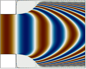
Figure 2(a,b) shows the spatial entropy distribution for two different frequencies as a solution of this advective equation. For both, the entropy presence expands after the expansion, but does so gradually, meaning that there is an annular region in the recirculation zone, delimited by the streamline passing through the separation point, where the entropy does not penetrate. This has important implications for the acoustic generation, since the entropy contribution to the source term in (3.1) is negligible in that region. To compute this source term, the gradient of the mean pressure is also required. Figure 2(c) shows that the mean pressure remains uniform upstream of the expansion and recovers along the length of the recirculation zone with the gradient in the axial direction being significantly larger than in the radial one. It remains almost constant immediately across the area expansion. The entropy-related source is thus concentrated within the expanding jet, with negligible presence in the recirculation ring.
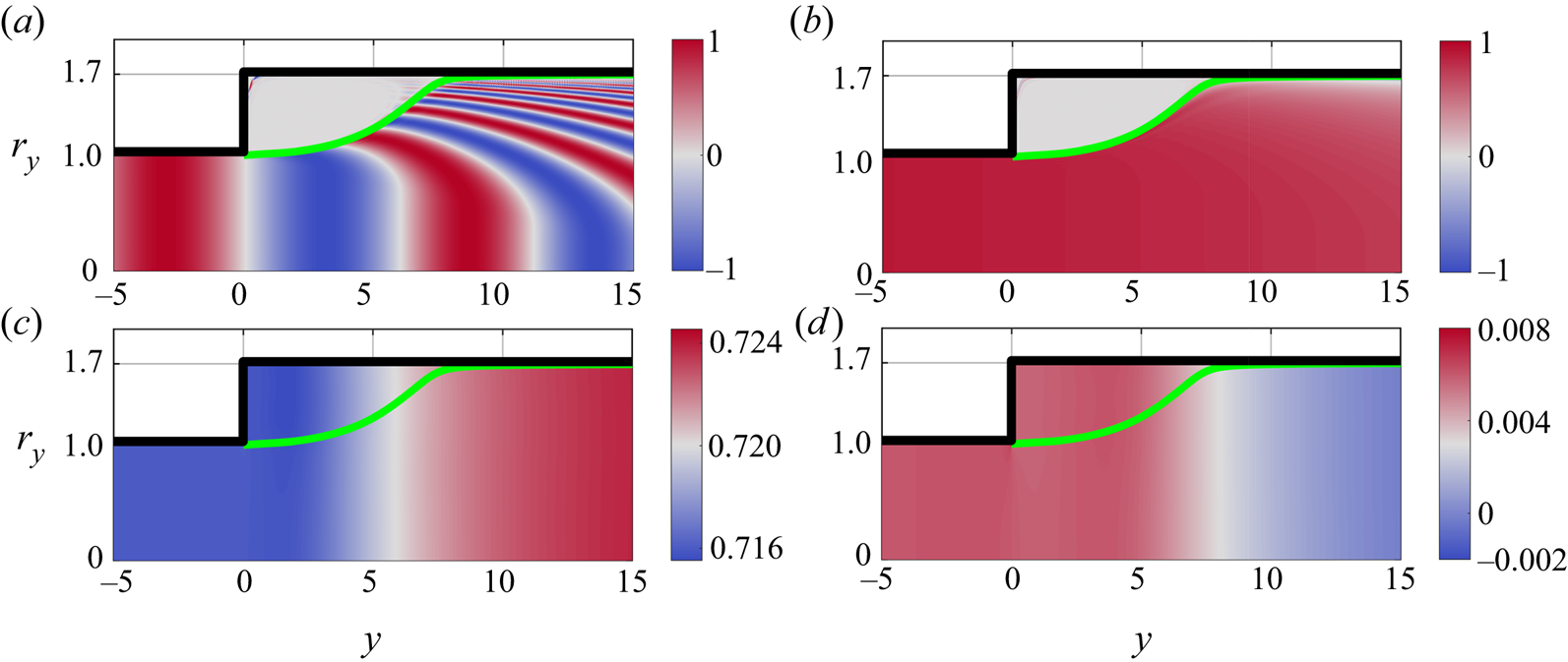
Figure 2. (a,b) Real part of the entropy perturbation for: (a)  $S_t= \omega R_u/\bar{u}_0 = 0.5$ and (b) $0.0125$ – results are from the bespoke simulation. (c) Mean pressure from RANS simulation and (d) real part of the perturbation pressure at $S_t=0.0125$ obtained by full LNSE simulations. The green line denotes the separation streamline.
This entropy-related source term is now combined with the Green's functions as described in § 3 to predict the reflected acoustic waves. Figure 3 shows predictions from the present model compared to the LNSE and the compact quasi-1-D isentropic model from Marble & Candel (Reference Marble and Candel1977, (31)). Note that the acoustic pressure perturbation is normalised by  $\gamma \bar{p}_0$ where $\gamma$ denotes the heat capacity ratio and $\bar{p}_0$ the mean pressure at the inlet, and the entropy perturbation is normalised by $c_p$. The Marble & Candel model assumes the expansion to be compact compared to both the acoustic and entropy wavelengths and, thus, has no frequency dependence. The LNSE predicts a nearly constant acoustic reflection amplitude when $St\leq 0.03$, but its value ( $\approx 0.007$) is much lower than that from Marble & Candel (Reference Marble and Candel1977) ( $\approx 0.016$). We want to emphasise that the LNSE numerical solver did predict the same reflection coefficient as Marble & Candel's model when a smooth contraction, with no flow separation, was considered. When $St>0.03$, non-compact effects cause a drop-off in the reflection coefficient amplitude in the form of a low-pass filter. Predictions from the present model closely match the low-frequency (compact) limit of the LNSE predictions, and also capture the fall-off at higher frequencies.
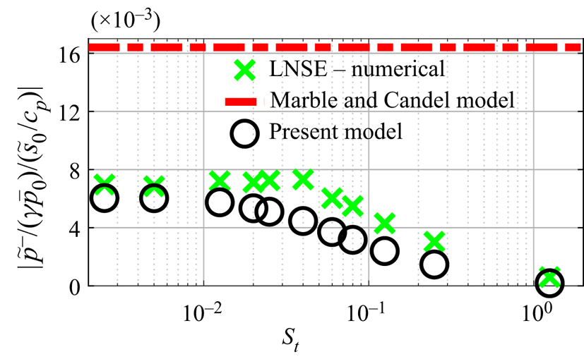
Figure 3. Acoustic reflection amplitudes predicted by the present model, the compact Marble & Candel (Reference Marble and Candel1977) model and the full LNSE simulations.
5. Simplified models
The physical mechanism causing the low-frequency acoustic reflection coefficient to differ substantially from that predicted by Marble & Candel (Reference Marble and Candel1977) remains unclear. Two simplified models are proposed in this section to further analyse this difference.
The first model, which we denote SimpM $1$, simplifies the entropy-related source term in (3.1). Figure 2 indicates that the source term is negligible inside the annular separation bubble and the mean pressure gradient is mainly in the axial direction (the radial gradient of $\bar {p}$ in (3.4) is negligible). At low frequencies, the entropy perturbation remains quasi-1-D. We thus assume a quasi-1-D mean flow profile within the given separation streamline (i.e. a nozzle geometry that follows the separation streamline). Additionally, this mean flow is assumed isentropic so that we can use the classical solutions for an isentropic 1-D nozzle. The entropy perturbation is then obtained from the 1-D advection equation $(\boldsymbol {i}\omega + \bar {u}(x) \textrm {d}/\textrm {d}\kern 0.05em x)\tilde {s}=0$. This greatly simplifies the entropy-related source term.
The second model, which we denote SimpM $2$, applies the simplifications of SimpM $1$, and further simplifies the Green's function in (3.4). An acoustic field is generated where there is flow deceleration, hence where the cross-sectional area occupied by the central jet varies. If the main jet expansion, and hence flow deceleration, occurs substantially beyond the area-increase interface, the generated higher-order acoustic modes decay before they reach the interface. We can then neglect all higher-order terms in the Green's function Bessel expansion and retain only the plane acoustic waves generated by the entropy-related source. This assumption is supported by the simulated pressure field in figure 2(d).
One would expect SimpM $1$ to recover Marble & Candel's compact quasi-1-D isentropic model if the frequency is low. However, we now show this to be true only if the axial extent of the recirculation zone is negligible. In order to artificially consider recirculation zones of different axial extents, an error function is used to model different separation streamlines, as shown in figure 4(a). A small standard deviation, $\epsilon =0.0001$, ensures a steep expansion at $y_{{mid}}$. Figure 4(b) shows that SimpM $1$ predictions tend to those from the Marble & Candel (Reference Marble and Candel1977) model only when $y_{{mid}}\lesssim 10^{-2}$. Beyond this value, the reflected acoustic wave amplitude falls off until it converges, at approximately $y_{{mid}}=1$, to the prediction from SimpM $2$. Thus, if the expansion of the central jet occurs an (upstream) radius or more beyond the expansion interface, the sound generated is very different to that predicted by the compact quasi-1-D isentropic model, even in the low-frequency (compact) limit. The sound is then accurately predicted by the simplest model, SimpM $2$.
$2$.
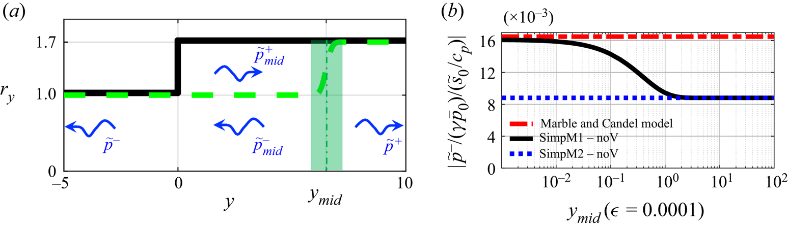
Figure 4. Effect of the axial extent of the recirculation zone on the acoustic response. (a) Green dashed line denotes a prescribed separation streamline for the central jet,  $r_y=1.35+0.35{\rm erf}[(y-y_{mid})/(\sqrt {2}\epsilon )]$ where $\textrm{erf}$ is the error function, and $\tilde {p}^{\pm }, \tilde {p}^{\pm }_{{mid}}$ are plane acoustic waves. (b) Reflected acoustic wave amplitude at $S_t=0.01$ against axial location of streamline expansion, $y_{mid}$: ‘noV’ denotes that the vortical sound source is neglected.
For real flows across significant area expansions, the recirculation zone usually extends far enough beyond the expansion plane that SimpM $2$ can be expected to provide good sound prediction. This is confirmed for the sudden expansion, now using the separation streamline from the RANS mean flow. Figure 5 shows that SimpM $1$ and SimpM $2$ predict very similar low-frequency acoustic reflection amplitudes, these being much closer to the LNSE results than those from the Marble & Candel model. They both also capture the higher-frequency fall-off, although with less accurate slope prediction than from the full model of figure 3. This suggests that, for the entropy-related source, 2-D effects become important at higher frequencies, consistent with visualisations in figure 2(a).
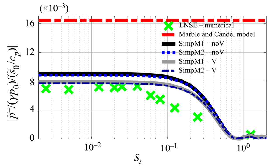
Figure 5. Reflected acoustic wave amplitude against Strouhal number using the RANS separation streamline: ‘noV’ and ‘V’ denote neglecting and accounting for vortical sound source, respectively.
Finally, both SimpM $1$ and SimpM $2$ can either neglect or account for the vorticity-related source term in (3.1). Figure 5 shows that accounting for it improves the predictions towards the LNSE results, but only slightly. This confirms that the entropy-related source is dominating over vorticity-related source, and that the size of the recirculation zone rather than flow non-isentropicity is the main factor causing different sound to that predicted by the quasi-1-D isentropic models.
6. Conclusions
The work makes two important contributions. Firstly, a new form of acoustic analogy is proposed that provides the first systematic derivation of the sound source terms due to entropy perturbations. This was achieved by revisiting Howe's acoustic analogy theory and carefully distinguishing acoustic perturbations from the entropy perturbation. At low Mach numbers and frequencies, the equation simplifies to an acoustic analogy in which acoustic propagation and acoustic source terms can be completely distinguished. Secondly, this governing equation was used to perform a quantitative study of the sound generated when entropy perturbations pass through a sudden flow expansion. The analogy was solved semi-analytically using a Green's function method and the acoustic reflection predictions were compared with those from both linearised Navier–Stokes equation simulations and quasi-1-D isentropic models. The comparisons showed, for the first time, that flow separation significantly changes entropy sound generation, leading both to a change in low-frequency (compact) behaviour and to a low-pass filter effect. This was shown to be mainly due to the spatial extent of the recirculation zone rather than non-isentropicity. It was also confirmed that, for the generated upstream propagating acoustic waves in the current case, the noise component associated with the vorticity shed at the separation point is subdominant in the sound generation process. Although not presented in the present paper, the downstream-travelling (transmitted) acoustic waves have also been calculated and modelled, with similar findings. The numerical (LNSE) predictions again differ to those from the Marble & Candel model, with the present simplified models able to capture the numerical predictions well. The interplay of the Kutta condition, the vorticity source term and the acoustic field is subtle in the present case, but could become more important at higher Mach numbers. An extension of the model to compare with recent experimental results (Rolland et al. Reference Rolland, De Domenico and Hochgreb2017), where entropy perturbations pass through a circular hole, is also under active studies by the authors.
Acknowledgements
The authors would like to gratefully acknowledge the European Research Council (ERC) Consolidator Grant AFIRMATIVE (2018–2023, grant number 772080) for supporting the current research.
Declaration of interests
The authors report no conflict of interest.


 Open access