


1. Introduction
Inertial focusing of particles suspended in flow through curved and spiral microfluidic ducts has been studied extensively in the experimental literature, particularly in relation to its application to size-based particle/cell separation (Seo, Lean & Kole Reference Seo, Lean and Kole2007; Bhagat, Kuntaegowdanahalli & Papautsky Reference Bhagat, Kuntaegowdanahalli and Papautsky2008; Di Carlo Reference Di Carlo2009; Martel & Toner Reference Martel and Toner2012; Warkiani et al. Reference Warkiani2014, Reference Warkiani, Khoo, Wu, Tay, Bhagat, Han and Lim2016; Rafeie et al. Reference Rafeie, Hosseinzadeh, Taylor and Warkiani2019). Much is known about the nature of the inertial lift force in a variety of situations involving a particle suspended in flow between two plane parallel walls (Saffman Reference Saffman1965; Ho & Leal Reference Ho and Leal1974; Schonberg & Hinch Reference Schonberg and Hinch1989; Hogg Reference Hogg1994; Asmolov Reference Asmolov1999). However, the nature of the inertial lift force is very different for a fully enclosed duct, making these studies of limited use in understanding practical applications. Sufficiently small particles suspended in flow through straight ducts with square cross-section are known to focus at one of four equilibria located a small distance from the centre of each sidewall (Di Carlo et al. Reference Di Carlo, Edd, Humphry, Stone and Toner2009; Hood, Lee & Roper Reference Hood, Lee and Roper2015). This is also the case for straight rectangular ducts, although stable equilibria near the shorter sidewalls attract relatively few particles and disappear entirely for larger particles (Martel & Toner Reference Martel and Toner2013; Hood Reference Hood2016). In curved ducts the migration of particles becomes complicated due to the secondary vortices that are generated as part of the Dean flow through the duct. The interaction of the drag force from these vortices with the inertial lift force leads to a wide variety of particle migration dynamics (Gossett & Di Carlo Reference Gossett and Di Carlo2009; Martel & Toner Reference Martel and Toner2014; Ha et al. Reference Ha, Harding, Bertozzi and Stokes2022; Valani, Harding & Stokes Reference Valani, Harding and Stokes2022).
Our previous study (Harding, Stokes & Bertozzi Reference Harding, Stokes and Bertozzi2019) conducted a detailed examination of the migration of neutrally buoyant spherical particles suspended in a sufficiently slow flow through curved rectangular ducts. An accurate model of particle migration was developed by coupling the particle motion to a Navier–Stokes model of the fluid flow. By using a carefully chosen reference frame, and applying a suitable non-dimensionalisation and perturbation expansion of both the background and disturbance flows, the individual forces primarily responsible for driving particle migration were separated and then estimated via numerical simulation. These forces were then re-assembled into a system of ordinary differential equations to model particle trajectories. It was found that particles migrated towards stable equilibria whose horizontal locations approximately collapsed onto a single curve when plotted against the parameter  $\kappa =\ell ^4/(4a^3R)$, with $\ell$ being the duct height, $a$ being the particle radius and $R$ being the bend radius. It was later shown how non-neutrally buoyant particles could be modelled by adding suitable perturbations to the neutrally buoyant model (Harding & Stokes Reference Harding and Stokes2020).
A key part of the prior modelling was an assumption that the flow rate is small enough that both  $\textit {Re}_{p}= 2\textit {Re}(a/\ell )^2$ and $K=\epsilon \textit {Re}^2$ are small, where $\epsilon =\ell /(2R)$ and $\textit {Re}=(\rho /\mu )U_m(\ell /2)$ is the channel Reynolds number with $\rho$ being the fluid density, $\mu$ the fluid viscosity and $U_m$ the maximum velocity of the background flow down the main axis. This allowed us to take the leading-order contribution of each perturbation expansion as a reasonable approximation. In a typical practical setting, these assumptions are somewhat limiting as they typically only hold when $\textit {Re}\lesssim {O}(10)$. In contrast, many microfluidics experiments in the literature operate at flow rates corresponding to $\textit {Re}={O}(100)$. While we expect our existing model may still have qualitative value at these flow rates, they are of less use quantitatively.
Substantially higher flow rates, e.g.  $\textit {Re}\gtrsim {O}(1000)$, are of limited practical interest for a few reasons. The first is that the increasing strength of the Dean flow eventually inhibits the ability of particles to focus, as seen in the decreasing sharpness factor with increasing flow rate in the experimental results of Rafeie et al. (Reference Rafeie, Hosseinzadeh, Taylor and Warkiani2019). Second, there is a critical Dean number, depending on the specific cross-section, above which the secondary component of the background flow exhibits multiple vortex pairs (Winters Reference Winters1987) and this seems generally undesirable for most applications. Third, the high pressures required to drive such high flow rates through microchannels cause practical difficulties, including excessive deformation of the channel geometry and difficulty maintaining connections.
In this paper we incorporate additional terms from the perturbation expansion of the background flow into the model. This has the effect of increasing the values of the Dean number  $K$ for which our model has quantitative value. Since we continue to use a leading-order approximation of the disturbance flow, this model does not expand the applicability in cases where the magnitude of $\textit {Re}_{p}$ is the limiting factor (e.g. when the particle is relatively large). Nonetheless, we feel this provides valuable insights and is an important step towards producing an accurate model applicable to a wide range of physical set-ups. This work also illustrates how the symmetry associated with a curved duct leads to a decoupling of axial and secondary components of the leading-order approximation of the disturbance flow which contribute to distinct inertial lift force components at first order.
Many of the classical analytical studies of inertial lift have utilised singular perturbation expansions rather than regular perturbation expansions, particularly those studies involving large Reynolds number flows. However, these studies have generally considered much simpler flow geometries, typically unidirectional flow between two plane parallel walls (Schonberg & Hinch Reference Schonberg and Hinch1989; Asmolov Reference Asmolov1999; Matas, Morris & Guazelli Reference Matas, Morris and Guazelli2004), or through a straight cylindrical pipe (Matas, Morris & Guazelli Reference Matas, Morris and Guazelli2009). In these set-ups, the problem can be reduced to solving a one-dimensional fourth-order ordinary differential equation. In more complex geometries, even just a straight square duct, this reduction is not possible. Consequently, the only way forward is a more direct computation of the outer solution, which needs to be matched appropriately to the inner solution. Moreover, the singular perturbation approach often requires special treatment in situations where the particle is not small relative to its separation from the nearest wall.
Given these challenges in utilising/implementing a singular perturbation based model, it is worth exploring the limits of what might be achieved with a regular perturbation. We acknowledge that our use of a regular perturbation expansion to study inertial migration at moderate Dean numbers is certainly pushing the boundaries of its applicability, but propose it is worth exploring in an effort to provide insights into how variations in the Dean number modify the inertial migration of particles. We have taken some care to discuss potential limitations of our model throughout the article.
The paper is organised as follows. Section 2 describes the general set-up of the problem and briefly summarises the modelling of forces driving particle migration as developed in Harding et al. (Reference Harding, Stokes and Bertozzi2019). We also introduce some notation to support the remainder of the text and remark on the applicability of the Lorentz reciprocal theorem to torque calculations. Section 3 describes our improved approximation of the background flow which utilises multiple terms from a perturbation expansion with respect to the Dean number  $K$. Section 4 describes how the new background flow approximation is incorporated into the inertial lift calculation and ultimately leads to a system of first-order differential equations which describe particle migration. The limitations of our model are also discussed. Section 5 reports a range of findings obtained from the new model: firstly, we examine how the horizontal locations of stable equilibria are perturbed by increasing $K$; secondly, we examine how varying $K$ influences previously observed trends in the horizontal location of stable equilibria with respect to $\epsilon ^{-1}$ and $\kappa$. Section 6 summarises our findings and remarks on avenues for future exploration.
2. Problem set-up and theoretical background
Our curved duct set-up remains identical to that in Harding et al. (Reference Harding, Stokes and Bertozzi2019) and is depicted in figure 1. The (stationary) laboratory reference frame is  $\boldsymbol {x}=x\boldsymbol {i}+y\boldsymbol {j}+z\boldsymbol {k}$ with the duct bending around the $z$-axis. The duct domain is most readily described using the cylindrical coordinate system $(r,\theta,z)$ for which
 \begin{equation} \boldsymbol{x}(r,\theta,z) = (R+r)\cos(\theta)\boldsymbol{i}+(R+r)\sin(\theta)\boldsymbol{j}+z\boldsymbol{k}, \end{equation}
where  $R$ is the (constant) bend radius of the duct measured from the origin (of the laboratory frame) to the centre of the cross-section. The cross-section itself is described by $(r,z)\in \mathcal {C}$ (with origin $(r,z)=(0,0)$ in the centre of the cross-section). The duct interior is then described by $\mathcal {D}=\{\boldsymbol {x}(\theta,r,z) \mid (r,z)\in \mathcal {C}\}$. While our approach can be applied to any desired cross-section $\mathcal {C}$, this study is concerned with rectangular cross-sections having width $W$ and height $H$, thus
 \begin{equation} \mathcal{C} = \left\{(r,z) : |r|\leq W/2,\ |z|\leq H/2 \right\}. \end{equation}
We take  $\ell =\min \{W,H\}$ to be the characteristic length scale of the duct. Of principal interest are ducts with $W\geq H$, and thus $\ell =H$, as these are most common in the experimental literature.
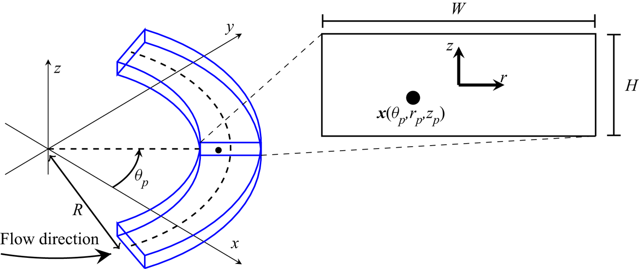
Figure 1. Curved duct with rectangular cross-section containing a spherical particle located at  $\boldsymbol {x}_{p}=\boldsymbol {x}(\theta _{p},r_{p},z_{p})$. The enlarged view of the cross-section containing the particle illustrates the origin of the local $r,z$ coordinates at the centre of the duct. The bend radius $R$ is with respect to the centerline of the duct. Note that we do not consider the flow near the inlet/outlet. Adapted from Harding et al. (Reference Harding, Stokes and Bertozzi2019).
Steady pressure driven flow through the duct (in the absence of particles) is referred to as the background flow. The fluid is assumed to be incompressible with constant density  $\rho$ and viscosity $\mu$. The pressure and velocity fields are denoted $\bar {p}$ and $\bar {\boldsymbol {u}}$, respectively, and are modelled using the Navier–Stokes equations. We take $U_{m}$ to be a characteristic velocity of this flow, approximately describing the maximum axial velocity. The channel/duct Reynolds number is then $\textit {Re}:=(\rho /\mu )U_{m}(\ell /2)$. Additionally, letting $\epsilon =\ell /(2R)$ denote the relative curvature, we define the Dean number as $K=\epsilon \textit {Re}^{2}$ after Dean (Reference Dean1927) and Dean & Hurst (Reference Dean and Hurst1959). The nature of the background flow, and its approximation for the purposes of this study, will be discussed further in § 3. Figure 2 depicts the axial (a) and secondary (b) components of the background flow, and (c) depicts the competing secondary drag and inertial lift forces on a particle.
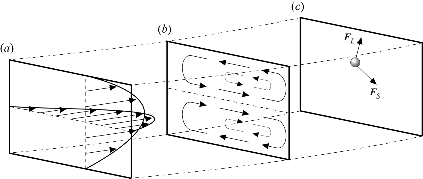
Figure 2. Cross-sections of a curved rectangular duct depicting (a) the axial component of the background flow; (b) the secondary component of the background flow consisting of two vertically symmetric counter-rotating vortices; (c) a spherical particle and the primary cross-sectional forces which drive its migration. Here,  $\boldsymbol {F}_{S}$ is the drag from the secondary component of the background flow, and $\boldsymbol {F}_{L}$ is the inertial lift force. The magnitude and direction of each vector are for illustration only. Gravitational and centrifugal/centripetal forces are omitted. The background flow is shown to be skewed towards the outside wall of the curved duct (here on the right), as is expected at moderate Dean numbers. Adapted from Harding & Stokes (Reference Harding and Stokes2020).
In this study we do not consider the fluid flow in a neighbourhood of the inlet nor outlet. Ault et al. (Reference Ault, Rallabandi, Shardt, Chen and Stone2017) studied the entry and exit flows in curved pipes and found that the entry length, taken to be the axial distance at which the velocity perturbation (from laminar flow) has decayed by 99 %, was  $0.0975\textit {Re}$ times the pipe diameter (independent of $\epsilon$). Based on this result, the total angle of the entry and exit regions for our curved ducts can be estimated as $22\textit {Re}\epsilon$ degrees. Given typical values of $\textit {Re}=100$ and $\epsilon =1/80$ then the total length of the entry and exit regions works out to be less than $1/12$ of complete revolution. Therefore, we conclude that the background flow is fully developed through the majority of a curved section that spans (close to) a complete revolution.
Now, consider a single particle suspended in the flow. Specifically, let  $\mathcal {P}:=\{\boldsymbol {x}:|\boldsymbol {x}-\boldsymbol {x}_{p}|< a\}$ denote a spherical particle centred at $\boldsymbol {x}_{p}(t)$ (such that $\mathcal {P}\subset \mathcal {D}$) having radius $a$ and constant density $\rho _{p}$. The cylindrical coordinates of its centre will be denoted by $r_p,\theta _p,z_p$, each a function of $t$. The particle travels with a velocity $\boldsymbol {u}_{p}(t):={\rm d}\boldsymbol {x}_{p}/{\rm d}t$ and spins freely about its centre with angular velocity $\boldsymbol {\varOmega }_{p}(t)$. Thus, each point $\boldsymbol {x}\in \mathcal {P}$ has instantaneous velocity $\boldsymbol {u}_{p}+\boldsymbol {\varOmega }_{p}\times (\boldsymbol {x}-\boldsymbol {x}_{p})$. The fluid domain is denoted $\mathcal {F}:=\mathcal {D}\backslash \mathcal {P}$ and its boundary $\partial \mathcal {F}$ consists of the duct walls $\partial \mathcal {D}$ and the particle surface $\partial \mathcal {P}$. The fluid flow is now described by the pressure and velocity fields $p,\boldsymbol {u}$, respectively, which are also modelled by the Navier–Stokes equations, specifically
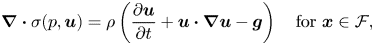 $$\begin{gather} \boldsymbol{\nabla}\boldsymbol{\cdot}\sigma(p,\boldsymbol{u}) = \rho\left(\frac{\partial\boldsymbol{u}}{\partial t}+\boldsymbol{u}\boldsymbol{\cdot} \boldsymbol{\nabla}\boldsymbol{u}-\boldsymbol{g}\right) \quad \text{for}\ \boldsymbol{x}\in\mathcal{F}, \end{gather}$$
 $$\begin{gather}\boldsymbol{\nabla}\boldsymbol{\cdot}\boldsymbol{u} = 0 \quad \text{for}\ \boldsymbol{x}\in\mathcal{F}, \end{gather}$$
 $$\begin{gather}\boldsymbol{u} = \boldsymbol{0} \quad \text{for}\ \boldsymbol{x}\in\partial\mathcal{D}, \end{gather}$$
 $$\begin{gather}\boldsymbol{u} = \boldsymbol{u}_{p}+\boldsymbol{\varOmega}_{p}\times(\boldsymbol{x}-\boldsymbol{x}_{p}) \quad \text{for}\ \boldsymbol{x}\in\partial\mathcal{P}, \end{gather}$$
where  $\sigma (p,\boldsymbol {u})$ is the stress tensor
 \begin{equation} \sigma(p,\boldsymbol{u}):={-}p{\mathsf{I}}+\mu\left(\boldsymbol{\nabla}\boldsymbol{u}+ \boldsymbol{\nabla}\boldsymbol{u}^{\intercal}\right). \end{equation}
 The gravitational body force  $\boldsymbol {g}$ is only important for non-neutrally buoyant particles ( $\rho _{p}\neq \rho$). In Harding & Stokes (Reference Harding and Stokes2020) it was demonstrated that with $\boldsymbol {g}=-g\boldsymbol {k}$ the influence of non-neutral buoyancy can be separated from the migration model and subsequently treated as an additional perturbation of the force experienced by a neutrally buoyant particle. This remains true in this study so we simplify the development by considering a neutrally buoyant particle (i.e. $\rho _{p}=\rho$) and drop the gravitational acceleration from (2.3a).
The motion of a suspended neutrally buoyant particle is driven solely by the hydrodynamic force and torque exerted on it. Specifically
 $$\begin{gather} \boldsymbol{F} := \int_{\partial\mathcal{P}}(-\boldsymbol{n}) \boldsymbol{\cdot}\sigma(p,\boldsymbol{u})\,{\rm d}S, \end{gather}$$
 $$\begin{gather}\boldsymbol{T} := \int_{\partial\mathcal{P}}(\boldsymbol{x}-\boldsymbol{x}_{p})\times \left((-\boldsymbol{n})\boldsymbol{\cdot}\sigma(p,\boldsymbol{u})\right){\rm d}S, \end{gather}$$
describe the force and torque, respectively, where  $\boldsymbol {n}$ is taken to be the normal with respect to the fluid domain (i.e. pointing in towards the particle centre).
The development of the migration model in Harding & Stokes (Reference Harding and Stokes2020) may be summarised as the following sequence of steps:
(i) Introduce a rotating reference frame in which the particle's angular coordinate is constant. This frame rotates with angular velocity $\boldsymbol {\varTheta }=\varTheta \boldsymbol {k}$ where $\varTheta :=\partial \theta _{p}/\partial t$. Coordinates in this rotating frame are mapped to the laboratory frame via
(2.6a)\begin{align} \boldsymbol{x}'(r',\theta',z') &= (R+r')\cos(\theta')\boldsymbol{i}'+(R+r') \sin(\theta')\boldsymbol{j}'+z'\boldsymbol{k} \end{align}(2.6b)where\begin{align} &=(R+r')\cos(\theta'+\theta_{p})\boldsymbol{i}+(R+r')\sin(\theta'+\theta_{p})\boldsymbol{j}+z'\boldsymbol{k}, \end{align}$\boldsymbol {i}':=\cos (\theta _{p})\boldsymbol {i}+\sin (\theta _{p})\boldsymbol {j}$ and $\,\boldsymbol {j}':=-\sin (\theta _{p})\boldsymbol {i}+\cos (\theta _{p})\boldsymbol {j}$. It follows that in the rotating frame $\boldsymbol {x}_{p}^{\prime }=\boldsymbol {x}'(r_{p},0,z_{p})$, $\boldsymbol {u}'=\boldsymbol {u}-\boldsymbol {\varTheta }\times \boldsymbol {x}$, $\bar {\boldsymbol {u}}'=\bar {\boldsymbol {u}}-\boldsymbol {\varTheta }\times \boldsymbol {x}$, and so on.
$\boldsymbol {\varTheta }=\varTheta \boldsymbol {k}$ where $\varTheta :=\partial \theta _{p}/\partial t$. Coordinates in this rotating frame are mapped to the laboratory frame via
(2.6a)\begin{align} \boldsymbol{x}'(r',\theta',z') &= (R+r')\cos(\theta')\boldsymbol{i}'+(R+r') \sin(\theta')\boldsymbol{j}'+z'\boldsymbol{k} \end{align}(2.6b)where\begin{align} &=(R+r')\cos(\theta'+\theta_{p})\boldsymbol{i}+(R+r')\sin(\theta'+\theta_{p})\boldsymbol{j}+z'\boldsymbol{k}, \end{align}$\boldsymbol {i}':=\cos (\theta _{p})\boldsymbol {i}+\sin (\theta _{p})\boldsymbol {j}$ and $\,\boldsymbol {j}':=-\sin (\theta _{p})\boldsymbol {i}+\cos (\theta _{p})\boldsymbol {j}$. It follows that in the rotating frame $\boldsymbol {x}_{p}^{\prime }=\boldsymbol {x}'(r_{p},0,z_{p})$, $\boldsymbol {u}'=\boldsymbol {u}-\boldsymbol {\varTheta }\times \boldsymbol {x}$, $\bar {\boldsymbol {u}}'=\bar {\boldsymbol {u}}-\boldsymbol {\varTheta }\times \boldsymbol {x}$, and so on.(ii) Assume the cross-sectional components of
$\boldsymbol {u}_{p}$ are sufficiently small that the flow in the rotating frame is approximately stationary and thus acceleration effects may be neglected (including added mass and Basset/history forces).(iii) Introduce the disturbance flow
$q',\boldsymbol {v}'$ which satisfies
(2.7a,b)\begin{equation} p'=\bar{p}'+q',\quad \boldsymbol{u}'=\bar{\boldsymbol{u}}'+\boldsymbol{v}'. \end{equation}(iv) Non-dimensionalise using the velocity scale
$U_{s}=(\alpha /2) U_{m}$ and length scale $a$, where $\alpha :=2a/\ell$. Most other scales may be derived from these (as per usual for a viscous flow). The resulting Reynolds number $\textit {Re}_{p}=(\rho /\mu )U_{s}a$ is often called the particle Reynolds number. The force on the particle is non-dimensionalised via the scale $\textit {Re}_{p}\mu U_{s}a$. Hats are used to describe non-dimensionalised variables, for example $\boldsymbol {v}'=U_{s}\hat {\boldsymbol {v}}'$.(v) Apply a perturbation expansion to the disturbance flow with respect to
$\textit {Re}_{p}$, that is
(2.8a,b)The force on the particle is expanded in a similar fashion, although the leading term has order\begin{equation} \hat{\boldsymbol{v}}' = \boldsymbol{v}_{0} + \textit{Re}_{p}\boldsymbol{v}_{1} + O(\textit{Re}_{p}^{2}),\quad \hat{q}' = q_{0} + \textit{Re}_{p} q_{1} + O(\textit{Re}_{p}^{2}). \end{equation}$\textit {Re}_{p}^{-1}$ and is denoted $\boldsymbol {F}_{-1}$ to reflect this, that is
(2.9)and similarly for the torque. Observe we drop both the hat and prime from variables upon applying the perturbation expansion to each of\begin{equation} \hat{\boldsymbol{F}}' = \textit{Re}_{p}^{{-}1}\boldsymbol{F}_{{-}1} + \boldsymbol{F}_{0} + O(\textit{Re}_{p}), \end{equation}$\hat {q}',\hat {\boldsymbol {v}}',\hat {\boldsymbol {F}}',\hat {\boldsymbol {T}}'$.


We take a moment to expand on the neglect of acceleration effects. As a particle migrates within the cross-section it not only has acceleration within this plane, but its axial velocity must also continuously adapt to that of the background flow. However, this study is primarily interested in the location of particle equilibria within the cross-section in regions of the duct where the background flow is fully developed. Once fully focused, the particle velocity and the net hydrodynamic force on the particle will be exactly zero (in the rotating frame). No acceleration effects can contribute to the force balance at this stage and, moreover, will be negligible in a neighbourhood of each equilibrium. Thus, such effects can be neglected for the purpose of locating and classifying equilibria.
Following the steps outlined above one arrives at the following equations governing  $q_{0},\boldsymbol {v}_{0}$:
 $$\begin{gather} \boldsymbol{\nabla}\boldsymbol{\cdot}\sigma(q_{0},\boldsymbol{v}_{0}) = \boldsymbol{0} \quad \text{for}\ \hat{\boldsymbol{x}}'\in\hat{\mathcal{F}}', \end{gather}$$
 $$\begin{gather}\boldsymbol{\nabla}\boldsymbol{\cdot}\boldsymbol{v}_{0} = 0 \quad \text{for}\ \hat{\boldsymbol{x}}'\in\hat{\mathcal{F}}', \end{gather}$$
 $$\begin{gather}\boldsymbol{v}_{0} = \boldsymbol{0} \quad \text{for}\ \hat{\boldsymbol{x}}'\in\partial\hat{\mathcal{D}}', \end{gather}$$
 $$\begin{gather}\boldsymbol{v}_{0}=\hat{\boldsymbol{u}}_{p,0}+\hat{\boldsymbol{\varOmega}}_{p,0}\times (\hat{\boldsymbol{x}}'-\hat{\boldsymbol{x}}_{p}^{\prime})-\widehat{\bar{\boldsymbol{u}}}\quad \text{for}\ \hat{\boldsymbol{x}}'\in\partial\hat{\mathcal{P}}'. \end{gather}$$
Similarly, one obtains the following equations governing  $q_{1},\boldsymbol {v}_{1}$:
 $$\begin{gather} \boldsymbol{\nabla}\boldsymbol{\cdot}\sigma(q_{1},\boldsymbol{v}_{1}) = \hat{\boldsymbol{\varTheta}}_0\times\boldsymbol{v}_{0}+\boldsymbol{v}_{0} \boldsymbol{\cdot}\boldsymbol{\nabla}\widehat{\bar{\boldsymbol{u}}}+ (\boldsymbol{v}_{0}+\widehat{\bar{\boldsymbol{u}}}-\hat{\boldsymbol{\varTheta}}_0\times \hat{\boldsymbol{x}}')\boldsymbol{\cdot} \boldsymbol{\nabla}\boldsymbol{v}_{0} \quad \text{for}\ \hat{\boldsymbol{x}}'\in\hat{\mathcal{F}}', \end{gather}$$
 $$\begin{gather}\boldsymbol{\nabla}\boldsymbol{\cdot}\boldsymbol{v}_{1} = 0 \quad \text{for}\ \hat{\boldsymbol{x}}'\in\hat{\mathcal{F}}', \end{gather}$$
 $$\begin{gather}\boldsymbol{v}_{1} = \boldsymbol{0} \quad \text{for}\ \hat{\boldsymbol{x}}'\in\partial\hat{\mathcal{D}}', \end{gather}$$
 $$\begin{gather}\boldsymbol{v}_{1} = \hat{\boldsymbol{u}}_{p,1}+\hat{\boldsymbol{\varOmega}}_{p,1}\times(\hat{\boldsymbol{x}}'-\hat{\boldsymbol{x}}_{p}^{\prime}) \quad \text{for}\ \hat{\boldsymbol{x}}'\in\partial\hat{\mathcal{P}}'. \end{gather}$$
Lastly, the force and torque terms of principal interest are
 \begin{gather} \boldsymbol{F}_{{-}1} = \int_{\partial\hat{\mathcal{P}}'}(-\boldsymbol{n}) \boldsymbol{\cdot}\sigma(q_{0},\boldsymbol{v}_{0})\,{\rm d}S, \end{gather}
 \begin{gather}\boldsymbol{T}_{{-}1} = \int_{\partial\hat{\mathcal{P}}'} (\hat{\boldsymbol{x}}'-\hat{\boldsymbol{x}}_{p}^{\prime})\times \left((-\boldsymbol{n})\boldsymbol{\cdot}\sigma(q_{0},\boldsymbol{v}_{0})\right){\rm d}S, \end{gather}
 \begin{align} \boldsymbol{F}_{0} &={-}\frac{4{\rm \pi}}{3}\hat{\boldsymbol{\varTheta}}_{0}\times (\hat{\boldsymbol{\varTheta}}_{0}\times\hat{\boldsymbol{x}}_{p}^{\prime}) -\frac{8{\rm \pi}}{3}\hat{\boldsymbol{\varTheta}}_{0}\times\hat{\boldsymbol{u}}_{p,0}^\prime +\int_{\hat{\mathcal{P}}'}\widehat{\bar{\boldsymbol{u}}}\boldsymbol{\cdot} \boldsymbol{\nabla}\widehat{\bar{\boldsymbol{u}}}\,{\rm d}V\nonumber\\ &\quad \ +\int_{\partial\hat{\mathcal{P}}'}(-\boldsymbol{n})\boldsymbol{\cdot} \sigma(q_{1},\boldsymbol{v}_{1})\,{\rm d}S, \end{align}
 \begin{align} \boldsymbol{T}_{0} &={-}\frac{8{\rm \pi}}{15}\hat{\boldsymbol{\varTheta}}_{0}\times \hat{\boldsymbol{\varOmega}}_{p,0}+\int_{\hat{\mathcal{P}}'} (\hat{\boldsymbol{x}}'-\hat{\boldsymbol{x}}_{p}^{\prime})\times (\widehat{\bar{\boldsymbol{u}}}\boldsymbol{\cdot} \boldsymbol{\nabla}\widehat{\bar{\boldsymbol{u}}})\,{\rm d}V \nonumber\\ &\quad \ +\int_{\partial\hat{\mathcal{P}}'}(\hat{\boldsymbol{x}}'-\hat{\boldsymbol{x}}_{p}^{\prime})\times \left[(-\boldsymbol{n})\boldsymbol{\cdot}\sigma(q_{1},\boldsymbol{v}_{1})\right]{\rm d}S. \end{align}
We refer the interested reader to Harding et al. (Reference Harding, Stokes and Bertozzi2019) for a complete derivation.
Note that in (2.10d) we retain a  $\hat {\boldsymbol {u}}_{p}$ contribution whereas in Harding et al. (Reference Harding, Stokes and Bertozzi2019) this was taken to be $\boldsymbol {\varTheta }\times \boldsymbol {x}_p^\prime$ (i.e. the $\theta$ component only) with drag coefficients associated with the cross-sectional components introduced later. Additionally, here we include particle velocity and spin contributions in (2.11d). Notice these contributions in both (2.10d) and (2.11d) are expressed in terms of $\hat {\boldsymbol {u}}_{p},\hat {\boldsymbol {\varOmega }}_{p}$ as viewed in the stationary reference frame. These minor changes allow us to separate the leading- and first-order contributions to the particle motion, and account for inertial lift contributions arising from the secondary component of the background flow.
It is reasonably well-known that the last term of (2.12c) can be computed without needing to explicitly calculate  $q_1,\boldsymbol {v}_1$ via an application of the Lorenz reciprocal theorem. Thus we only need to consider the solution of (2.10). Before moving on to describe our improved background flow approximation, we introduce some additional notation and make a remark about the use of the Lorentz reciprocal theorem.
2.1. Stokes’ flow operators
We introduce the operators  $\mathcal {Q}(\boldsymbol {f}),\boldsymbol {\mathcal {V}}(\boldsymbol {f})$ which map a continuous vector field $\boldsymbol {f}$ defined on the particle surface $\partial \hat {\mathcal {P}}'$ to a pressure and velocity field, respectively, which satisfies the Stokes’ equations
 $$\begin{gather} \boldsymbol{\nabla}\boldsymbol{\cdot}\sigma \left(\mathcal{Q}(\boldsymbol{f}),\boldsymbol{\mathcal{V}}(\boldsymbol{f})\right) = \boldsymbol{0} \quad \text{for}\ \hat{\boldsymbol{x}}'\in\hat{\mathcal{F}}', \end{gather}$$
 $$\begin{gather}\boldsymbol{\nabla}\boldsymbol{\cdot}\boldsymbol{\mathcal{V}}(\boldsymbol{f}) = 0 \quad \text{for}\ \hat{\boldsymbol{x}}'\in\hat{\mathcal{F}}', \end{gather}$$
 $$\begin{gather}\boldsymbol{\mathcal{V}}(\boldsymbol{f}) = \boldsymbol{0} \quad \text{for}\ \hat{\boldsymbol{x}}'\in\partial\hat{\mathcal{D}}', \end{gather}$$
 $$\begin{gather}\boldsymbol{\mathcal{V}}(\boldsymbol{f}) = \boldsymbol{f} \quad \text{for}\ \hat{\boldsymbol{x}}'\in\partial\hat{\mathcal{P}}'. \end{gather}$$
Additionally, maps from  $\boldsymbol {f}$ to the corresponding hydrodynamic force and torque on the particle are denoted by the operators
 $$\begin{gather} \boldsymbol{\mathcal{M}}(\boldsymbol{f}) := \int_{\partial\hat{\mathcal{P}}'} (-\boldsymbol{n})\boldsymbol{\cdot}\sigma(\mathcal{Q}(\boldsymbol{f}), \boldsymbol{\mathcal{V}}(\boldsymbol{f}))\,{\rm d}S, \end{gather}$$
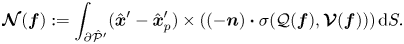 $$\begin{gather}\boldsymbol{\mathcal{N}}(\boldsymbol{f}) := \int_{\partial\hat{\mathcal{P}}'} (\hat{\boldsymbol{x}}'-\hat{\boldsymbol{x}}_{p}^{\prime})\times\left((-\boldsymbol{n}) \boldsymbol{\cdot}\sigma(\mathcal{Q}(\boldsymbol{f}), \boldsymbol{\mathcal{V}}(\boldsymbol{f}))\right){\rm d}S. \end{gather}$$
When  $\boldsymbol {f}$ is a constant unit vector then $\boldsymbol {\mathcal {M}}(\boldsymbol {f})$ and $\boldsymbol {\mathcal {N}}(\boldsymbol {f})$ may be interpreted as force and torque coefficients, respectively, in the direction of $\boldsymbol {f}$. Note that all four of these operators implicitly depend on the location of the particle within the cross-section since the fluid domain $\hat {\mathcal {F}}'$ and particle boundary $\partial \hat {\mathcal {P}}'$ depend on $\hat {r}_p,\hat {z}_p$. Additionally, there is an implicit dependence on $\epsilon$, as this relates to the bend radius of the duct, and $\alpha$, as this relates to the size of the non-dimensionalised fluid domain. The implicit dependence on $\epsilon$ is expected to be very weak for $\epsilon < 1/10$, as will be illustrated in § 3.
Observe that the operators  $\mathcal {Q},\boldsymbol {\mathcal {V}},\boldsymbol {\mathcal {M}},\boldsymbol {\mathcal {N}}$ are linear and therefore we may write
 $$\begin{gather} q_{0} =\mathcal{Q}(\hat{\boldsymbol{u}}_{p,0})+\mathcal{Q}(\hat{\boldsymbol{\varOmega}}_{p,0} \times(\hat{\boldsymbol{x}}'-\hat{\boldsymbol{x}}_{p}^{\prime}))-\mathcal{Q}(\widehat{\bar{\boldsymbol{u}}}), \end{gather}$$
 $$\begin{gather}\boldsymbol{v}_{0} =\boldsymbol{\mathcal{V}}(\hat{\boldsymbol{u}}_{p,0})+\boldsymbol{\mathcal{V}} (\hat{\boldsymbol{\varOmega}}_{p,0}\times(\hat{\boldsymbol{x}}'-\hat{\boldsymbol{x}}_{p}^{\prime}))- \boldsymbol{\mathcal{V}}(\widehat{\bar{\boldsymbol{u}}}), \end{gather}$$
 $$\begin{gather}\boldsymbol{F}_{{-}1} =\boldsymbol{\mathcal{M}}(\hat{\boldsymbol{u}}_{p,0})+ \boldsymbol{\mathcal{M}}(\hat{\boldsymbol{\varOmega}}_{p,0}\times(\hat{\boldsymbol{x}}'-\hat{\boldsymbol{x}}_{p}^{\prime}))- \boldsymbol{\mathcal{M}}(\widehat{\bar{\boldsymbol{u}}}), \end{gather}$$
 $$\begin{gather}\boldsymbol{T}_{{-}1} =\boldsymbol{\mathcal{N}}(\hat{\boldsymbol{u}}_{p,0})+\boldsymbol{\mathcal{N}} (\hat{\boldsymbol{\varOmega}}_{p,0}\times(\hat{\boldsymbol{x}}'-\hat{\boldsymbol{x}}_{p}^{\prime}))- \boldsymbol{\mathcal{N}}(\widehat{\bar{\boldsymbol{u}}}). \end{gather}$$
The linearity will be further exploited in § 4. Appendix B describes when various components of these coefficients are zero due to the axisymmetry of our domain.
2.2. A note on reciprocal theorems
A variant of the Lorentz reciprocal theorem can be applied to show that
 \begin{align} \int_{\partial\hat{\mathcal{P}}'}(-\boldsymbol{n})\boldsymbol{\cdot} \sigma(q_{1},\boldsymbol{v}_{1})\,{\rm d}S &= \boldsymbol{\mathcal{M}}(\hat{\boldsymbol{u}}_{p,1})+\boldsymbol{\mathcal{M}}(\hat{\boldsymbol{\varOmega}}_{p,1} \times(\hat{\boldsymbol{x}}'-\hat{\boldsymbol{x}}_{p}^{\prime})) \nonumber\\ &\quad -\sum_{\boldsymbol{e}\in\{\boldsymbol{i}',\,\boldsymbol{j}',\,\boldsymbol{k}\}}\boldsymbol{e} \int_{\hat{\mathcal{F}}'}\boldsymbol{\mathcal{V}}(\boldsymbol{e})\boldsymbol{\cdot}\boldsymbol{I}_{0}\,{\rm d}V, \end{align}
where  $\boldsymbol {I}_{0}$ is the right side of (2.11a), that is
 \begin{equation} \boldsymbol{I}_{0} := \hat{\boldsymbol{\varTheta}}_{0}\times\boldsymbol{v}_{0}+\boldsymbol{v}_{0}\boldsymbol{\cdot} \boldsymbol{\nabla}\widehat{\bar{\boldsymbol{u}}}+(\boldsymbol{v}_{0}+ \widehat{\bar{\boldsymbol{u}}}-\hat{\boldsymbol{\varTheta}}_{0}\times\hat{\boldsymbol{x}}') \boldsymbol{\cdot}\boldsymbol{\nabla}\boldsymbol{v}_{0}. \end{equation}
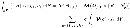
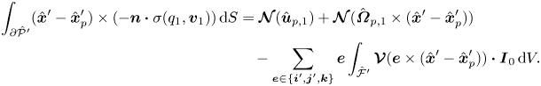
This application of the Lorentz reciprocal theorem to the calculation of the inertial lift force is reasonably well known. Perhaps less well known is that it can also be applied to the calculation of the torque terms. Specifically, the third term of  $\boldsymbol {T}_{0}$ in (2.12d) can be calculated via
 \begin{align}
\int_{\partial\hat{\mathcal{P}}'}(\hat{\boldsymbol{x}}'-\hat{\boldsymbol{x}}_{p}^{\prime})\times
\left(-\boldsymbol{n}\boldsymbol{\cdot}\sigma(q_{1},\boldsymbol{v}_{1})\right){\rm
d}S &= \boldsymbol{\mathcal{N}}(\hat{\boldsymbol{u}}_{p,1})
+\boldsymbol{\mathcal{N}}(\hat{\boldsymbol{\varOmega}}_{p,1}
\times(\hat{\boldsymbol{x}}'-\hat{\boldsymbol{x}}_{p}^{\prime}))
\nonumber\\ &\quad
-\sum_{\boldsymbol{e}\in\{\boldsymbol{i}',\boldsymbol{j}',\boldsymbol{k}\}}\boldsymbol{e}\int_{\hat{\mathcal{F}}'}
\boldsymbol{\mathcal{V}}(\boldsymbol{e}\times(\hat{\boldsymbol{x}}'-\hat{\boldsymbol{x}}_{p}^{\prime}))
\boldsymbol{\cdot}\boldsymbol{I}_{0}\,{\rm d}V.
\end{align}
\begin{align}
\int_{\partial\hat{\mathcal{P}}'}(\hat{\boldsymbol{x}}'-\hat{\boldsymbol{x}}_{p}^{\prime})\times
\left(-\boldsymbol{n}\boldsymbol{\cdot}\sigma(q_{1},\boldsymbol{v}_{1})\right){\rm
d}S &= \boldsymbol{\mathcal{N}}(\hat{\boldsymbol{u}}_{p,1})
+\boldsymbol{\mathcal{N}}(\hat{\boldsymbol{\varOmega}}_{p,1}
\times(\hat{\boldsymbol{x}}'-\hat{\boldsymbol{x}}_{p}^{\prime}))
\nonumber\\ &\quad
-\sum_{\boldsymbol{e}\in\{\boldsymbol{i}',\boldsymbol{j}',\boldsymbol{k}\}}\boldsymbol{e}\int_{\hat{\mathcal{F}}'}
\boldsymbol{\mathcal{V}}(\boldsymbol{e}\times(\hat{\boldsymbol{x}}'-\hat{\boldsymbol{x}}_{p}^{\prime}))
\boldsymbol{\cdot}\boldsymbol{I}_{0}\,{\rm d}V.
\end{align}
Notice that the  $\boldsymbol {\mathcal {M}}$ and $\boldsymbol {\mathcal {N}}$ terms in (2.16) and (2.18), respectively, encapsulate the contributions from the boundary conditions (2.11d), while the remaining volume integrals are the result of the reciprocal theorem applied to capture the contribution of $\boldsymbol {I}_{0}$. For completeness, a proof of the reciprocal theorems that give rise to (2.16) and (2.18) is provided in Appendix A.
3. Improved approximation of the background flow
The background flow  $\bar {p},\bar {\boldsymbol {u}}$ is a steady solution of the Navier–Stokes equations
 $$\begin{gather} \boldsymbol{\nabla}\boldsymbol{\cdot}\sigma(\bar{p},\boldsymbol{\bar{u}}) = \rho\bar{\boldsymbol{u}}\boldsymbol{\cdot}\boldsymbol{\nabla} \bar{\boldsymbol{u}} \quad \boldsymbol{x}\in\mathcal{D}, \end{gather}$$
 $$\begin{gather}\boldsymbol{\nabla}\boldsymbol{\cdot}\bar{\boldsymbol{u}} = 0 \quad \boldsymbol{x}\in\mathcal{D}, \end{gather}$$
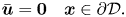 $$\begin{gather}\bar{\boldsymbol{u}} = \boldsymbol{0} \quad \boldsymbol{x}\in\partial\mathcal{D}. \end{gather}$$
The resulting velocity field may be decomposed into its axial component  $\bar {\boldsymbol {u}}_a$ and secondary component $\bar {\boldsymbol {u}}_s$. A perturbation expansion may be applied to each component with respect to $K=\epsilon \textit {Re}^2$ which converges provided $K\lesssim 212$ (Harding Reference Harding2019d). Specifically
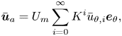 $$\begin{gather} \bar{\boldsymbol{u}}_a = U_m\sum_{i=0}^{\infty}K^i\bar{u}_{\theta,i}\boldsymbol{e}_{\theta}, \end{gather}$$
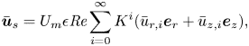 $$\begin{gather}\bar{\boldsymbol{u}}_s = U_m\epsilon\textit{Re}\sum_{i=0}^{\infty}K^i(\bar{u}_{r,i}\boldsymbol{e}_{r}+\bar{u}_{z,i}\boldsymbol{e}_{z}), \end{gather}$$
where  $\bar {u}_{\theta,i},\bar {u}_{r,i},\bar {u}_{z,i}$ are the (dimensionless) components of $\bar {\boldsymbol {u}}$ in the $\theta,r,z$ directions, respectively, and are each independent of $\theta$.
Our previous model used only the leading-order terms  $\bar {u}_{\theta,0},\bar {u}_{r,0},\bar {u}_{z,0}$ to model inertial migration in curved ducts based on an assumption that $K$ is suitably small (Harding et al. Reference Harding, Stokes and Bertozzi2019). In this study we extend the use of (3.2) to accurately model particle migration for values of $K$ up to $O(100)$. Specifically, we use the three leading terms $i=0,1,2$ to construct a model of particle migration which is quadratic in $K$. Upon non-dimensionalising with respect to the shear velocity scale ( $U_s=(\alpha /2) U_m=(a/\ell )U_m$) our model may be expressed as
 \begin{equation}
\widehat{\bar{\boldsymbol{u}}}\approx 2\alpha^{{-}1}
(\bar{\boldsymbol{u}}_{a,0}+K\bar{\boldsymbol{u}}_{a,1}+K^{2}\bar{\boldsymbol{u}}_{a,2})
+\kappa\textit{Re}_{p}(\bar{\boldsymbol{u}}_{s,0}+K\bar{\boldsymbol{u}}_{s,1}+K^2
\bar{\boldsymbol{u}}_{s,2}),
\end{equation}
\begin{equation}
\widehat{\bar{\boldsymbol{u}}}\approx 2\alpha^{{-}1}
(\bar{\boldsymbol{u}}_{a,0}+K\bar{\boldsymbol{u}}_{a,1}+K^{2}\bar{\boldsymbol{u}}_{a,2})
+\kappa\textit{Re}_{p}(\bar{\boldsymbol{u}}_{s,0}+K\bar{\boldsymbol{u}}_{s,1}+K^2
\bar{\boldsymbol{u}}_{s,2}),
\end{equation}
where  $\bar {\boldsymbol {u}}_{a,i}:=\bar {u}_{\theta,i}\boldsymbol {e}_{\theta }$ and $\bar {\boldsymbol {u}}_{s,i}:=\bar {u}_{r,i}\boldsymbol {e}_{r}+\bar {u}_{z,i}\boldsymbol {e}_{z}$ for each $i$. Notice in (3.3) we have used the fact that $2\alpha ^{-1}\epsilon \textit {Re}=\kappa \textit {Re}_p$ (recalling $\kappa =\ell ^{4}/(4a^3R)$).
We illustrate the accuracy of our improved model of the background flow in figure 3. We use the streamfunction  $\bar {\varPhi }$, for which $\bar {u}_{r}=-(1+\epsilon r)^{-1}\partial \bar {\varPhi }/\partial z$ and $\bar {u}_{z}=(1+\epsilon r)^{-1}\partial \bar {\varPhi }/\partial r$, for the purpose of evaluating the accuracy of the secondary components. Figure 3(a) illustrates the accuracy of our quadratic model over the range $1\leq K\leq 200$ using a fixed aspect ratio $W/H=2$ and curvature parameter $\epsilon =0.01$. Here, the notation $\bar {u}_{\theta \mid i},\bar {\varPhi }_{\mid i}$ indicates the approximation (3.2) is truncated beyond the $i'$th term. In each case the relative $L_2$ error is proportional to $K^{i+1}$. Observe that the approximations $\bar {u}_{\theta \mid 1},\bar {\varPhi }_{\mid 1}$ and $\bar {u}_{\theta \mid 2},\bar {\varPhi }_{\mid 2}$ are significant improvements over $\bar {u}_{\theta \mid 0},\bar {\varPhi }_{\mid 0}$ for $K=O(10)$. Additionally, for $K=O(100)$ the approximation $\bar {u}_{\theta \mid 2},\bar {\varPhi }_{\mid 2}$ offers a marginal improvement over $\bar {u}_{\theta \mid 1},\bar {\varPhi }_{\mid 1}$. When $K=100$ the relative errors are $0.95\,\%$ for $\bar {u}_{\theta \mid 2}$ and $2.05\,\%$ for $\bar {\varPhi }_{\mid 2}$. This illustrates that the first three terms are a reasonable trade-off between computational cost and achieving a reasonably accurate model for $K=O(100)$.
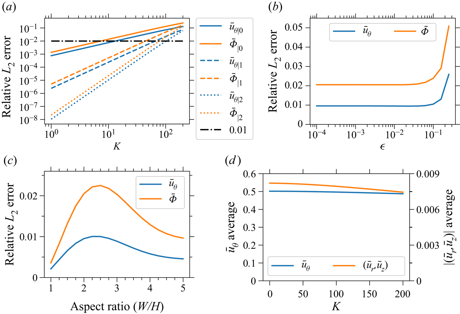
Figure 3. The relative  $L_{2}$ error of truncated perturbation approximations of $\bar {u}_{\theta }$ and $\bar {\varPhi }$ vs (a) the Dean number $K\in [1,200]$, (b) the relative curvature $\epsilon \in [10^{-4},0.25]$ and (c) the cross-section aspect ratio $W/H\in [1,5]$. (d) Shows the change in the average of $\bar {u}_{\theta }$ and $|(\bar {u}_{r},\bar {u}_{z})|$ vs $K\in [0,200]$. Parameters are: (a) $W/H=2$ and $\epsilon =0.01$; (b) $W/H=2$ and $K=100$; (c) $K=100$ and $\epsilon =0.01$; (d) $W/H=2$ and $\epsilon =0.01$.
For the remainder of the discussion we take  $\bar {u}_{\theta }=\bar {u}_{\theta \mid 2}$ and similarly $\bar {\varPhi }=\bar {\varPhi }_{\mid 2}$. Figure 3(b) shows how the model error changes with respect to the $\epsilon$ parameter, using fixed $K=100$ and aspect ratio $W/H=2$. It is evident that the accuracy of the approximation is roughly the same across all ducts having a fixed bend radius for which $\epsilon <1/10$. In other words, the model accuracy is insensitive to $\epsilon$ provided it is not too large. Figure 3(c) shows the variation in model error with respect to aspect ratio of the cross-section, using fixed $K=100$ and $\epsilon =0.01$. While there is some dependence of the model error on the aspect ratio, the case $W/H=2$ is near the peak for aspect ratios $W/H\geq 1$ and is therefore a reasonable choice of reference value.
We take a moment to elaborate on the choice of characteristic velocity  $U_m$ used in this study. The pressure gradient which drives flow through the curved duct increases super-linearly with the flow rate and also has a (weak) dependence on the bend radius. Given a $K>0$, determining the pressure gradient which produces the required flow rate becomes a nonlinear optimisation problem. The nonlinearity is weak over the range of $K$ considered in this study and therefore it will be convenient to avoid the nonlinear optimisation. To this end, we specify the characteristic velocity $U_m$ to be the maximum velocity of a laminar flow through a straight duct having an identical cross-section. This is equivalent to non-dimensionalising with respect to the driving pressure gradient, since straight duct flow satisfies Stokes’ equation and therefore does not depend on the Reynolds number, that is $U_m=c_{\mathcal {C}}G\ell ^2/\mu$, where $G$ is the pressure gradient down the main flow axis and $c_{\mathcal {C}}$ is a constant depending only on the cross-section $\mathcal {C}$. This choice makes it straightforward to compare results across different duct bend radii and incorporate $K$ as a new parameter in our inertial migration model. Figure 3(d) illustrates how the average of the non-dimensional $\bar {u}_\theta$ and $\bar {\varPhi }$ varies as a function of $K$ for our specific non-dimensionalisation, with fixed $\epsilon =0.01$ and $W/H=2$. The average of $\bar {u}_\theta$ is approximately constant over this range of $K$ indicating that our specific choice of characteristic velocity is easily translated to an average axial flow rate if desired.
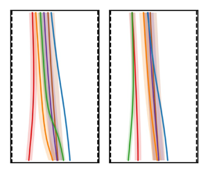
Figure 4 illustrates the difference in features of the fields  $\bar {u}_\theta,\bar {\varPhi }$ between $K=0$ to $K=100$. Note that $K=0$ should be interpreted as the limit $K\to 0$ as a result of a decaying flow rate $U_m$. While the physical magnitude of the secondary vortices decays to zero as $U_m\to 0$ our specific non-dimensionalisation of $\bar {\boldsymbol {u}}_s$, via the scaling $U_m\epsilon \textit {Re}$ in (3.2b), ensures that the magnitude of the secondary vortices remains finite. Observe in figure 4 a shift of local maxima and minima towards the outside/right wall when $K=100$. This is due to the increased rotational inertia of the fluid and is not captured by the leading-order approximation of the background flow used in Harding et al. (Reference Harding, Stokes and Bertozzi2019). This shift becomes more pronounced with further increases in $K$. Lastly, we point out that the Dean numbers $K\lesssim 200$ considered herein are significantly smaller than the critical Dean number after which there exist four vortex solutions (Winters Reference Winters1987).

Figure 4. The fields (a,c)  $\bar {u}_\theta$ and (b,d) $\bar {\varPhi }$ for (a,b) $K=0$ and (c,d) $K=100$. In each case $\epsilon =0.01$ and $W/H=2$. The colour bars have been fixed across the pairs (a,c) and (b,d) for comparison.
4. The extended particle migration model
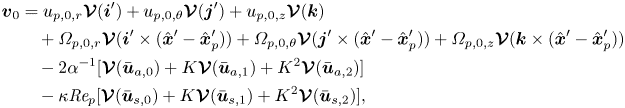
Here, we incorporate the improved approximation of the background flow (3.3) into the model so that we may efficiently approximate particle trajectories for any desired  $0\leq K\lesssim 200$. We start by decomposing the leading-order disturbance flow $q_{0},\boldsymbol {v}_{0}$ further than was previously done in Harding et al. (Reference Harding, Stokes and Bertozzi2019). Doing so reveals how the axial and secondary components of the background flow influence all six components of $\hat {\boldsymbol {u}}_{p},\hat {\boldsymbol {\varOmega }}_{p}$ at both leading and first order. Additionally, we illustrate that the decomposition admits a decoupling which can be exploited to more efficiently compute all the non-zero forces and torques. Finally, we summarise the complete model and its limitations.
4.1. Further decomposition and application of symmetry
Utilising the operator  $\boldsymbol {\mathcal {V}}$, and expanding further on (2.15), observe that $\boldsymbol {v}_{0}$ can be decomposed as
 \begin{align}
\boldsymbol{v}_{0} &=
u_{p,0,r}\boldsymbol{\mathcal{V}}(\boldsymbol{i}')
+u_{p,0,\theta}\boldsymbol{\mathcal{V}}(\boldsymbol{j}')+u_{p,0,z}\boldsymbol{\mathcal{V}}(\boldsymbol{k})
\nonumber\\ &\quad
+\varOmega_{p,0,r}\boldsymbol{\mathcal{V}}(\boldsymbol{i}'\times(\hat{\boldsymbol{x}}'-\hat{\boldsymbol{x}}_{p}^{\prime}))+
\varOmega_{p,0,\theta}\boldsymbol{\mathcal{V}}(\boldsymbol{j}'\times(\hat{\boldsymbol{x}}'-\hat{\boldsymbol{x}}_{p}^{\prime}))+
\varOmega_{p,0,z}\boldsymbol{\mathcal{V}}(\boldsymbol{k}\times(\hat{\boldsymbol{x}}'-\hat{\boldsymbol{x}}_{p}^{\prime}))
\nonumber\\ &\quad
-2\alpha^{{-}1}[\boldsymbol{\mathcal{V}}(\bar{\boldsymbol{u}}_{a,0})+K\boldsymbol{\mathcal{V}}(\bar{\boldsymbol{u}}_{a,1})+
K^{2}\boldsymbol{\mathcal{V}}(\bar{\boldsymbol{u}}_{a,2})]
\nonumber\\ &\quad
-\kappa\textit{Re}_{p}[\boldsymbol{\mathcal{V}}(\bar{\boldsymbol{u}}_{s,0})
+K\boldsymbol{\mathcal{V}}
(\bar{\boldsymbol{u}}_{s,1})+K^{2}\boldsymbol{\mathcal{V}}(\bar{\boldsymbol{u}}_{s,2})],
\end{align}
\begin{align}
\boldsymbol{v}_{0} &=
u_{p,0,r}\boldsymbol{\mathcal{V}}(\boldsymbol{i}')
+u_{p,0,\theta}\boldsymbol{\mathcal{V}}(\boldsymbol{j}')+u_{p,0,z}\boldsymbol{\mathcal{V}}(\boldsymbol{k})
\nonumber\\ &\quad
+\varOmega_{p,0,r}\boldsymbol{\mathcal{V}}(\boldsymbol{i}'\times(\hat{\boldsymbol{x}}'-\hat{\boldsymbol{x}}_{p}^{\prime}))+
\varOmega_{p,0,\theta}\boldsymbol{\mathcal{V}}(\boldsymbol{j}'\times(\hat{\boldsymbol{x}}'-\hat{\boldsymbol{x}}_{p}^{\prime}))+
\varOmega_{p,0,z}\boldsymbol{\mathcal{V}}(\boldsymbol{k}\times(\hat{\boldsymbol{x}}'-\hat{\boldsymbol{x}}_{p}^{\prime}))
\nonumber\\ &\quad
-2\alpha^{{-}1}[\boldsymbol{\mathcal{V}}(\bar{\boldsymbol{u}}_{a,0})+K\boldsymbol{\mathcal{V}}(\bar{\boldsymbol{u}}_{a,1})+
K^{2}\boldsymbol{\mathcal{V}}(\bar{\boldsymbol{u}}_{a,2})]
\nonumber\\ &\quad
-\kappa\textit{Re}_{p}[\boldsymbol{\mathcal{V}}(\bar{\boldsymbol{u}}_{s,0})
+K\boldsymbol{\mathcal{V}}
(\bar{\boldsymbol{u}}_{s,1})+K^{2}\boldsymbol{\mathcal{V}}(\bar{\boldsymbol{u}}_{s,2})],
\end{align}
where  $\hat {\boldsymbol {u}}_{p,0}=(u_{p,0,r},u_{p,0,\theta },u_{p,0,z})$ and $\hat {\boldsymbol {\varOmega }}_{p,0}=(\varOmega _{p,0,r},\varOmega _{p,0,\theta },\varOmega _{p,0,z})$. This expansion extracts all of the key parameters from the leading disturbance solution making it a linear superposition of Stokes flow solutions.
Notice that the last line of (4.1) has a factor  $\textit {Re}_p$ and could therefore be placed in $\boldsymbol {v}_{1}$ (which would be equivalent to moving the appropriate component of the boundary condition in (2.10d) to (2.11d)). However, in many practical situations $\kappa \gg 1$ and thus $\kappa \textit {Re}_p$ may not be small. Consequently, it will be convenient to keep these terms in $\boldsymbol {v}_0$. An expansion identical to (4.1) is obtained for each of $q_{0}$, $\boldsymbol {F}_{-1}$ and $\boldsymbol {T}_{-1}$ by replacing each $\boldsymbol {\mathcal {V}}$ with $\mathcal {Q}$, $\boldsymbol {\mathcal {M}}$ and $\boldsymbol {\mathcal {N}}$, respectively.
Upon setting  $\boldsymbol {F}_{-1}=\boldsymbol {0}$ and $\boldsymbol {T}_{-1}=\boldsymbol {0}$, one obtains six equations which are linear with respect to the six components of $\boldsymbol {u}_{p,0},\boldsymbol {\varOmega }_{p,0}$. Applying the symmetry properties described in Appendix B allows the $6\times 6$ system to be decoupled into two distinct $3\times 3$ systems. One of these describes the equilibrium attained by the particle parameters $u_{p,0,\theta },\varOmega _{p,0,r},\varOmega _{p,0,z}$ in relation to the axial motion of the background flow
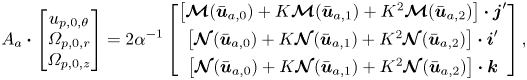 \begin{equation} A_a
\boldsymbol{\cdot}\begin{bmatrix} u_{p,0,\theta} \\ \varOmega_{p,0,r}
\\ \varOmega_{p,0,z} \end{bmatrix}=2\alpha^{{-}1}
\begin{bmatrix}
\left[\boldsymbol{\mathcal{M}}(\bar{\boldsymbol{u}}_{a,0})+K\boldsymbol{\mathcal{M}}(\bar{\boldsymbol{u}}_{a,1})+K^{2}\boldsymbol{\mathcal{M}}(\bar{\boldsymbol{u}}_{a,2})\right]\boldsymbol{\cdot}\boldsymbol{j}'
\\
\left[\boldsymbol{\mathcal{N}}(\bar{\boldsymbol{u}}_{a,0})+K\boldsymbol{\mathcal{N}}(\bar{\boldsymbol{u}}_{a,1})+K^{2}\boldsymbol{\mathcal{N}}(\bar{\boldsymbol{u}}_{a,2})\right]\boldsymbol{\cdot}\boldsymbol{i}'
\\
\left[\boldsymbol{\mathcal{N}}(\bar{\boldsymbol{u}}_{a,0})+K\boldsymbol{\mathcal{N}}(\bar{\boldsymbol{u}}_{a,1})+K^{2}\boldsymbol{\mathcal{N}}(\bar{\boldsymbol{u}}_{a,2})\right]\boldsymbol{\cdot}\boldsymbol{k}
\end{bmatrix}, \end{equation}
\begin{equation} A_a
\boldsymbol{\cdot}\begin{bmatrix} u_{p,0,\theta} \\ \varOmega_{p,0,r}
\\ \varOmega_{p,0,z} \end{bmatrix}=2\alpha^{{-}1}
\begin{bmatrix}
\left[\boldsymbol{\mathcal{M}}(\bar{\boldsymbol{u}}_{a,0})+K\boldsymbol{\mathcal{M}}(\bar{\boldsymbol{u}}_{a,1})+K^{2}\boldsymbol{\mathcal{M}}(\bar{\boldsymbol{u}}_{a,2})\right]\boldsymbol{\cdot}\boldsymbol{j}'
\\
\left[\boldsymbol{\mathcal{N}}(\bar{\boldsymbol{u}}_{a,0})+K\boldsymbol{\mathcal{N}}(\bar{\boldsymbol{u}}_{a,1})+K^{2}\boldsymbol{\mathcal{N}}(\bar{\boldsymbol{u}}_{a,2})\right]\boldsymbol{\cdot}\boldsymbol{i}'
\\
\left[\boldsymbol{\mathcal{N}}(\bar{\boldsymbol{u}}_{a,0})+K\boldsymbol{\mathcal{N}}(\bar{\boldsymbol{u}}_{a,1})+K^{2}\boldsymbol{\mathcal{N}}(\bar{\boldsymbol{u}}_{a,2})\right]\boldsymbol{\cdot}\boldsymbol{k}
\end{bmatrix}, \end{equation}
where
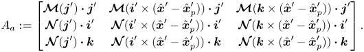 \begin{equation} A_a := \begin{bmatrix}
\boldsymbol{\mathcal{M}}(\boldsymbol{j}')\boldsymbol{\cdot}\boldsymbol{j}'
&
\boldsymbol{\mathcal{M}}(\boldsymbol{i}'\times(\hat{\boldsymbol{x}}'-\hat{\boldsymbol{x}}_{p}^{\prime}))\boldsymbol{\cdot}\boldsymbol{j}'
&
\boldsymbol{\mathcal{M}}(\boldsymbol{k}\times(\hat{\boldsymbol{x}}'-\hat{\boldsymbol{x}}_{p}^{\prime}))\boldsymbol{\cdot}\boldsymbol{j}'
\\
\boldsymbol{\mathcal{N}}(\boldsymbol{j}')\boldsymbol{\cdot}\boldsymbol{i}'
&
\boldsymbol{\mathcal{N}}(\boldsymbol{i}'\times(\hat{\boldsymbol{x}}'-\hat{\boldsymbol{x}}_{p}^{\prime}))\boldsymbol{\cdot}\boldsymbol{i}'
&
\boldsymbol{\mathcal{N}}(\boldsymbol{k}\times(\hat{\boldsymbol{x}}'-\hat{\boldsymbol{x}}_{p}^{\prime}))\boldsymbol{\cdot}\boldsymbol{i}'
\\
\boldsymbol{\mathcal{N}}(\boldsymbol{j}')\boldsymbol{\cdot}\boldsymbol{k}
&
\boldsymbol{\mathcal{N}}(\boldsymbol{i}'\times(\hat{\boldsymbol{x}}'-\hat{\boldsymbol{x}}_{p}^{\prime}))\boldsymbol{\cdot}\boldsymbol{k}
&
\boldsymbol{\mathcal{N}}(\boldsymbol{k}\times(\hat{\boldsymbol{x}}'-\hat{\boldsymbol{x}}_{p}^{\prime}))\boldsymbol{\cdot}\boldsymbol{k}
\end{bmatrix}. \end{equation}
\begin{equation} A_a := \begin{bmatrix}
\boldsymbol{\mathcal{M}}(\boldsymbol{j}')\boldsymbol{\cdot}\boldsymbol{j}'
&
\boldsymbol{\mathcal{M}}(\boldsymbol{i}'\times(\hat{\boldsymbol{x}}'-\hat{\boldsymbol{x}}_{p}^{\prime}))\boldsymbol{\cdot}\boldsymbol{j}'
&
\boldsymbol{\mathcal{M}}(\boldsymbol{k}\times(\hat{\boldsymbol{x}}'-\hat{\boldsymbol{x}}_{p}^{\prime}))\boldsymbol{\cdot}\boldsymbol{j}'
\\
\boldsymbol{\mathcal{N}}(\boldsymbol{j}')\boldsymbol{\cdot}\boldsymbol{i}'
&
\boldsymbol{\mathcal{N}}(\boldsymbol{i}'\times(\hat{\boldsymbol{x}}'-\hat{\boldsymbol{x}}_{p}^{\prime}))\boldsymbol{\cdot}\boldsymbol{i}'
&
\boldsymbol{\mathcal{N}}(\boldsymbol{k}\times(\hat{\boldsymbol{x}}'-\hat{\boldsymbol{x}}_{p}^{\prime}))\boldsymbol{\cdot}\boldsymbol{i}'
\\
\boldsymbol{\mathcal{N}}(\boldsymbol{j}')\boldsymbol{\cdot}\boldsymbol{k}
&
\boldsymbol{\mathcal{N}}(\boldsymbol{i}'\times(\hat{\boldsymbol{x}}'-\hat{\boldsymbol{x}}_{p}^{\prime}))\boldsymbol{\cdot}\boldsymbol{k}
&
\boldsymbol{\mathcal{N}}(\boldsymbol{k}\times(\hat{\boldsymbol{x}}'-\hat{\boldsymbol{x}}_{p}^{\prime}))\boldsymbol{\cdot}\boldsymbol{k}
\end{bmatrix}. \end{equation}
The diagonal elements of  $A_a$ are negative and generally the matrix is diagonally dominant. Recall that each $\boldsymbol {\mathcal {M}}$ and $\boldsymbol {\mathcal {N}}$ term implicitly depends on $\epsilon,\alpha$ and the cross-sectional coordinates of the particle $(\hat {r}_{p},\hat {z}_{p})$. Solving (4.2) therefore yields an expression for each of $u_{p,0,\theta },\varOmega _{p,0,r},\varOmega _{p,0,z}$ which depend only on the parameters $\hat {r}_{p},\hat {z}_{p},\epsilon,\alpha,K$.
The remaining  $3\times 3$ system describes the equilibrium attained by the particle parameters $u_{p,r},u_{p,z},\varOmega _{p,\theta }$ in relation to the secondary motion of the background flow
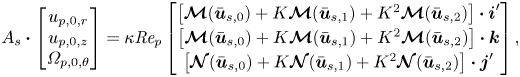 \begin{equation} A_s \boldsymbol{\cdot}
\begin{bmatrix} u_{p,0,r} \\ u_{p,0,z} \\
\varOmega_{p,0,\theta}
\end{bmatrix}=\kappa\textit{Re}_{p}\begin{bmatrix}
\left[\boldsymbol{\mathcal{M}}(\bar{\boldsymbol{u}}_{s,0})+K\boldsymbol{\mathcal{M}}(\bar{\boldsymbol{u}}_{s,1})+K^{2}\boldsymbol{\mathcal{M}}(\bar{\boldsymbol{u}}_{s,2})\right]\boldsymbol{\cdot}\boldsymbol{i}'
\\
\left[\boldsymbol{\mathcal{M}}(\bar{\boldsymbol{u}}_{s,0})+K\boldsymbol{\mathcal{M}}(\bar{\boldsymbol{u}}_{s,1})+K^{2}\boldsymbol{\mathcal{M}}(\bar{\boldsymbol{u}}_{s,2})\right]\boldsymbol{\cdot}\boldsymbol{k}
\\
\left[\boldsymbol{\mathcal{N}}(\bar{\boldsymbol{u}}_{s,0})+K\boldsymbol{\mathcal{N}}(\bar{\boldsymbol{u}}_{s,1})+K^{2}\boldsymbol{\mathcal{N}}(\bar{\boldsymbol{u}}_{s,2})\right]\boldsymbol{\cdot}\boldsymbol{j}'
\end{bmatrix}, \end{equation}
\begin{equation} A_s \boldsymbol{\cdot}
\begin{bmatrix} u_{p,0,r} \\ u_{p,0,z} \\
\varOmega_{p,0,\theta}
\end{bmatrix}=\kappa\textit{Re}_{p}\begin{bmatrix}
\left[\boldsymbol{\mathcal{M}}(\bar{\boldsymbol{u}}_{s,0})+K\boldsymbol{\mathcal{M}}(\bar{\boldsymbol{u}}_{s,1})+K^{2}\boldsymbol{\mathcal{M}}(\bar{\boldsymbol{u}}_{s,2})\right]\boldsymbol{\cdot}\boldsymbol{i}'
\\
\left[\boldsymbol{\mathcal{M}}(\bar{\boldsymbol{u}}_{s,0})+K\boldsymbol{\mathcal{M}}(\bar{\boldsymbol{u}}_{s,1})+K^{2}\boldsymbol{\mathcal{M}}(\bar{\boldsymbol{u}}_{s,2})\right]\boldsymbol{\cdot}\boldsymbol{k}
\\
\left[\boldsymbol{\mathcal{N}}(\bar{\boldsymbol{u}}_{s,0})+K\boldsymbol{\mathcal{N}}(\bar{\boldsymbol{u}}_{s,1})+K^{2}\boldsymbol{\mathcal{N}}(\bar{\boldsymbol{u}}_{s,2})\right]\boldsymbol{\cdot}\boldsymbol{j}'
\end{bmatrix}, \end{equation}
where
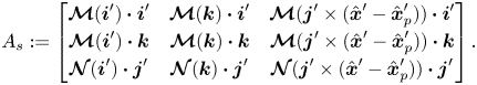 \begin{equation} A_s := \begin{bmatrix}
\boldsymbol{\mathcal{M}}(\boldsymbol{i}')\boldsymbol{\cdot}\boldsymbol{i}'
&
\boldsymbol{\mathcal{M}}(\boldsymbol{k})\boldsymbol{\cdot}\boldsymbol{i}'
&
\boldsymbol{\mathcal{M}}(\boldsymbol{j}'\times(\hat{\boldsymbol{x}}'-\hat{\boldsymbol{x}}_{p}^{\prime}))\boldsymbol{\cdot}\boldsymbol{i}'
\\
\boldsymbol{\mathcal{M}}(\boldsymbol{i}')\boldsymbol{\cdot}\boldsymbol{k}
&
\boldsymbol{\mathcal{M}}(\boldsymbol{k})\boldsymbol{\cdot}\boldsymbol{k}
&
\boldsymbol{\mathcal{M}}(\boldsymbol{j}'\times(\hat{\boldsymbol{x}}'-\hat{\boldsymbol{x}}_{p}^{\prime}))\boldsymbol{\cdot}\boldsymbol{k}
\\
\boldsymbol{\mathcal{N}}(\boldsymbol{i}')\boldsymbol{\cdot}\boldsymbol{j}'
&
\boldsymbol{\mathcal{N}}(\boldsymbol{k})\boldsymbol{\cdot}\boldsymbol{j}'
&
\boldsymbol{\mathcal{N}}(\boldsymbol{j}'\times(\hat{\boldsymbol{x}}'-\hat{\boldsymbol{x}}_{p}^{\prime}))\boldsymbol{\cdot}\boldsymbol{j}'
\end{bmatrix}. \end{equation}
\begin{equation} A_s := \begin{bmatrix}
\boldsymbol{\mathcal{M}}(\boldsymbol{i}')\boldsymbol{\cdot}\boldsymbol{i}'
&
\boldsymbol{\mathcal{M}}(\boldsymbol{k})\boldsymbol{\cdot}\boldsymbol{i}'
&
\boldsymbol{\mathcal{M}}(\boldsymbol{j}'\times(\hat{\boldsymbol{x}}'-\hat{\boldsymbol{x}}_{p}^{\prime}))\boldsymbol{\cdot}\boldsymbol{i}'
\\
\boldsymbol{\mathcal{M}}(\boldsymbol{i}')\boldsymbol{\cdot}\boldsymbol{k}
&
\boldsymbol{\mathcal{M}}(\boldsymbol{k})\boldsymbol{\cdot}\boldsymbol{k}
&
\boldsymbol{\mathcal{M}}(\boldsymbol{j}'\times(\hat{\boldsymbol{x}}'-\hat{\boldsymbol{x}}_{p}^{\prime}))\boldsymbol{\cdot}\boldsymbol{k}
\\
\boldsymbol{\mathcal{N}}(\boldsymbol{i}')\boldsymbol{\cdot}\boldsymbol{j}'
&
\boldsymbol{\mathcal{N}}(\boldsymbol{k})\boldsymbol{\cdot}\boldsymbol{j}'
&
\boldsymbol{\mathcal{N}}(\boldsymbol{j}'\times(\hat{\boldsymbol{x}}'-\hat{\boldsymbol{x}}_{p}^{\prime}))\boldsymbol{\cdot}\boldsymbol{j}'
\end{bmatrix}. \end{equation}
Similar to  $A_a$, the diagonal elements of $A_s$ are negative and generally the matrix is diagonally dominant.
We now consider the balance of force and torque at the next order of  $\textit {Re}_p$ by setting $\boldsymbol {F}_{0}=\boldsymbol {0}$ and $\boldsymbol {T}_{0}=\boldsymbol {0}$. The symmetries that lead to (4.2) and (4.4) analogously lead to
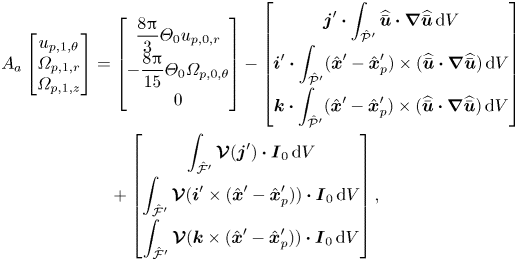 \begin{align} A_a\begin{bmatrix}
u_{p,1,\theta} \\ \varOmega_{p,1,r} \\ \varOmega_{p,1,z}
\end{bmatrix} &= \begin{bmatrix}
\dfrac{8{\rm \pi}}{3}\varTheta_0 u_{p,0,r} \\
-\dfrac{8{\rm \pi}}{15}\varTheta_{0}\varOmega_{p,0,\theta} \\ 0
\end{bmatrix} -\begin{bmatrix}
\boldsymbol{j}'\boldsymbol{\cdot}\displaystyle\int_{\hat{\mathcal{P}}'}\widehat{\bar{\boldsymbol{u}}}\boldsymbol{\cdot}\boldsymbol{\nabla}\widehat{\bar{\boldsymbol{u}}}\,{\rm
d}V \\
\boldsymbol{i}'\boldsymbol{\cdot}\displaystyle\int_{\hat{\mathcal{P}}'}(\hat{\boldsymbol{x}}'-\hat{\boldsymbol{x}}_{p}^{\prime})\times(\widehat{\bar{\boldsymbol{u}}}\boldsymbol{\cdot}\boldsymbol{\nabla}\widehat{\bar{\boldsymbol{u}}})\,{\rm
d}V \\
\boldsymbol{k}\boldsymbol{\cdot}\displaystyle\int_{\hat{\mathcal{P}}'}(\hat{\boldsymbol{x}}'-\hat{\boldsymbol{x}}_{p}^{\prime})\times(\widehat{\bar{\boldsymbol{u}}}\boldsymbol{\cdot}\boldsymbol{\nabla}\widehat{\bar{\boldsymbol{u}}})\,{\rm
d}V \end{bmatrix} \nonumber\\ &\quad +\begin{bmatrix}
\displaystyle\int_{\hat{\mathcal{F}}'}\boldsymbol{\mathcal{V}}(\boldsymbol{j}')\boldsymbol{\cdot}\boldsymbol{I}_{0}\,{\rm
d}V \\
\displaystyle\int_{\hat{\mathcal{F}}'}\boldsymbol{\mathcal{V}}(\boldsymbol{i}'\times(\hat{\boldsymbol{x}}'-\hat{\boldsymbol{x}}_{p}^{\prime}))\boldsymbol{\cdot}\boldsymbol{I}_{0}\,{\rm
d}V \\
\displaystyle\int_{\hat{\mathcal{F}}'}\boldsymbol{\mathcal{V}}(\boldsymbol{k}\times(\hat{\boldsymbol{x}}'-\hat{\boldsymbol{x}}_{p}^{\prime}))\boldsymbol{\cdot}\boldsymbol{I}_{0}\,{\rm
d}V \end{bmatrix}, \end{align}
\begin{align} A_a\begin{bmatrix}
u_{p,1,\theta} \\ \varOmega_{p,1,r} \\ \varOmega_{p,1,z}
\end{bmatrix} &= \begin{bmatrix}
\dfrac{8{\rm \pi}}{3}\varTheta_0 u_{p,0,r} \\
-\dfrac{8{\rm \pi}}{15}\varTheta_{0}\varOmega_{p,0,\theta} \\ 0
\end{bmatrix} -\begin{bmatrix}
\boldsymbol{j}'\boldsymbol{\cdot}\displaystyle\int_{\hat{\mathcal{P}}'}\widehat{\bar{\boldsymbol{u}}}\boldsymbol{\cdot}\boldsymbol{\nabla}\widehat{\bar{\boldsymbol{u}}}\,{\rm
d}V \\
\boldsymbol{i}'\boldsymbol{\cdot}\displaystyle\int_{\hat{\mathcal{P}}'}(\hat{\boldsymbol{x}}'-\hat{\boldsymbol{x}}_{p}^{\prime})\times(\widehat{\bar{\boldsymbol{u}}}\boldsymbol{\cdot}\boldsymbol{\nabla}\widehat{\bar{\boldsymbol{u}}})\,{\rm
d}V \\
\boldsymbol{k}\boldsymbol{\cdot}\displaystyle\int_{\hat{\mathcal{P}}'}(\hat{\boldsymbol{x}}'-\hat{\boldsymbol{x}}_{p}^{\prime})\times(\widehat{\bar{\boldsymbol{u}}}\boldsymbol{\cdot}\boldsymbol{\nabla}\widehat{\bar{\boldsymbol{u}}})\,{\rm
d}V \end{bmatrix} \nonumber\\ &\quad +\begin{bmatrix}
\displaystyle\int_{\hat{\mathcal{F}}'}\boldsymbol{\mathcal{V}}(\boldsymbol{j}')\boldsymbol{\cdot}\boldsymbol{I}_{0}\,{\rm
d}V \\
\displaystyle\int_{\hat{\mathcal{F}}'}\boldsymbol{\mathcal{V}}(\boldsymbol{i}'\times(\hat{\boldsymbol{x}}'-\hat{\boldsymbol{x}}_{p}^{\prime}))\boldsymbol{\cdot}\boldsymbol{I}_{0}\,{\rm
d}V \\
\displaystyle\int_{\hat{\mathcal{F}}'}\boldsymbol{\mathcal{V}}(\boldsymbol{k}\times(\hat{\boldsymbol{x}}'-\hat{\boldsymbol{x}}_{p}^{\prime}))\boldsymbol{\cdot}\boldsymbol{I}_{0}\,{\rm
d}V \end{bmatrix}, \end{align}
and similarly
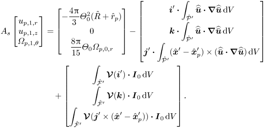 \begin{align} A_s \begin{bmatrix}
u_{p,1,r} \\ u_{p,1,z} \\ \varOmega_{p,1,\theta}
\end{bmatrix} &= \begin{bmatrix}
-\dfrac{4{\rm \pi}}{3}\varTheta_{0}^{2}(\hat{R}+\hat{r}_{p}) \\
0 \\ \dfrac{8{\rm \pi}}{15}\varTheta_{0}\varOmega_{p,0,r}
\end{bmatrix}-\begin{bmatrix}
\boldsymbol{i}'\boldsymbol{\cdot}\displaystyle\int_{\hat{\mathcal{P}}'}\widehat{\bar{\boldsymbol{u}}}\boldsymbol{\cdot}\boldsymbol{\nabla}\widehat{\bar{\boldsymbol{u}}}\,{\rm
d}V \\
\boldsymbol{k}\boldsymbol{\cdot}\displaystyle\int_{\hat{\mathcal{P}}'}\widehat{\bar{\boldsymbol{u}}}\boldsymbol{\cdot}\boldsymbol{\nabla}\widehat{\bar{\boldsymbol{u}}}\,{\rm
d}V \\
\boldsymbol{j}'\boldsymbol{\cdot}\displaystyle\int_{\hat{\mathcal{P}}'}(\hat{\boldsymbol{x}}'-\hat{\boldsymbol{x}}_{p}^{\prime})\times(\widehat{\bar{\boldsymbol{u}}}\boldsymbol{\cdot}\boldsymbol{\nabla}\widehat{\bar{\boldsymbol{u}}})\,{\rm
d}V \end{bmatrix} \nonumber\\ &\quad +\begin{bmatrix}
\displaystyle\int_{\hat{\mathcal{F}}'}\boldsymbol{\mathcal{V}}(\boldsymbol{i}')\boldsymbol{\cdot}\boldsymbol{I}_{0}
\,{\rm d}V \\
\displaystyle\int_{\hat{\mathcal{F}}'}\boldsymbol{\mathcal{V}}(\boldsymbol{k})\boldsymbol{\cdot}\boldsymbol{I}_{0}
\,{\rm d}V \\
\displaystyle\int_{\hat{\mathcal{F}}'}\boldsymbol{\mathcal{V}}(\boldsymbol{j}'\times(\hat{\boldsymbol{x}}'-\hat{\boldsymbol{x}}_{p}^{\prime}))\boldsymbol{\cdot}\boldsymbol{I}_{0}\,{\rm
d}V \end{bmatrix}. \end{align}
\begin{align} A_s \begin{bmatrix}
u_{p,1,r} \\ u_{p,1,z} \\ \varOmega_{p,1,\theta}
\end{bmatrix} &= \begin{bmatrix}
-\dfrac{4{\rm \pi}}{3}\varTheta_{0}^{2}(\hat{R}+\hat{r}_{p}) \\
0 \\ \dfrac{8{\rm \pi}}{15}\varTheta_{0}\varOmega_{p,0,r}
\end{bmatrix}-\begin{bmatrix}
\boldsymbol{i}'\boldsymbol{\cdot}\displaystyle\int_{\hat{\mathcal{P}}'}\widehat{\bar{\boldsymbol{u}}}\boldsymbol{\cdot}\boldsymbol{\nabla}\widehat{\bar{\boldsymbol{u}}}\,{\rm
d}V \\
\boldsymbol{k}\boldsymbol{\cdot}\displaystyle\int_{\hat{\mathcal{P}}'}\widehat{\bar{\boldsymbol{u}}}\boldsymbol{\cdot}\boldsymbol{\nabla}\widehat{\bar{\boldsymbol{u}}}\,{\rm
d}V \\
\boldsymbol{j}'\boldsymbol{\cdot}\displaystyle\int_{\hat{\mathcal{P}}'}(\hat{\boldsymbol{x}}'-\hat{\boldsymbol{x}}_{p}^{\prime})\times(\widehat{\bar{\boldsymbol{u}}}\boldsymbol{\cdot}\boldsymbol{\nabla}\widehat{\bar{\boldsymbol{u}}})\,{\rm
d}V \end{bmatrix} \nonumber\\ &\quad +\begin{bmatrix}
\displaystyle\int_{\hat{\mathcal{F}}'}\boldsymbol{\mathcal{V}}(\boldsymbol{i}')\boldsymbol{\cdot}\boldsymbol{I}_{0}
\,{\rm d}V \\
\displaystyle\int_{\hat{\mathcal{F}}'}\boldsymbol{\mathcal{V}}(\boldsymbol{k})\boldsymbol{\cdot}\boldsymbol{I}_{0}
\,{\rm d}V \\
\displaystyle\int_{\hat{\mathcal{F}}'}\boldsymbol{\mathcal{V}}(\boldsymbol{j}'\times(\hat{\boldsymbol{x}}'-\hat{\boldsymbol{x}}_{p}^{\prime}))\boldsymbol{\cdot}\boldsymbol{I}_{0}\,{\rm
d}V \end{bmatrix}. \end{align}
Here,  $\hat {R}=R/a$ and $\varTheta _0=(\hat {R}+\hat {r}_p)u_{p,0,\theta }$ (such that $\varTheta _0\boldsymbol {k}=\boldsymbol {\varTheta }_{0}$). In previous studies the corrections $u_{p,1,\theta },\boldsymbol {\varOmega }_{p,1}$ and off-diagonal elements of $A_a,A_s$ were ignored. The net contribution from the first two vectors on the right side of each of (4.6) and (4.7) is typically small and can be ignored, however, they have been included here for completeness.
4.2. The completed model
Using the result of the four equations (4.2), (4.4), (4.6) and (4.7) our complete migration model is
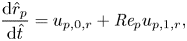 $$\begin{gather} \frac{{\rm d} \hat{r}_p}{{\rm d}\hat{t}} = u_{p,0,r}+\textit{Re}_{p}u_{p,1,r}, \end{gather}$$
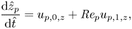 $$\begin{gather}\frac{{\rm d} \hat{z}_p}{{\rm d}\hat{t}} = u_{p,0,z}+\textit{Re}_{p}u_{p,1,z}, \end{gather}$$
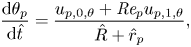 $$\begin{gather}\frac{{\rm d} \theta_p}{{\rm d}\hat{t}} = \frac{u_{p,0,\theta}+\textit{Re}_{p}u_{p,1,\theta}}{\hat{R}+\hat{r}_{p}}, \end{gather}$$
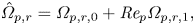 $$\begin{gather}\hat{\varOmega}_{p,r} = \varOmega_{p,r,0}+\textit{Re}_{p}\varOmega_{p,r,1}, \end{gather}$$
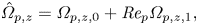 $$\begin{gather}\hat{\varOmega}_{p,z} = \varOmega_{p,z,0}+\textit{Re}_{p}\varOmega_{p,z,1}, \end{gather}$$
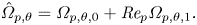 $$\begin{gather}\hat{\varOmega}_{p,\theta} = \varOmega_{p,\theta,0}+\textit{Re}_{p}\varOmega_{p,\theta,1}. \end{gather}$$
Appendix C describes further simplifications that can be made to (4.6) and (4.7) owing to symmetries about the plane  $\theta '=0$. These result in the alternative equations (C4) and (C5) which provide additional insight into the interplay between axial and secondary flow components and their influence on the first-order terms $\boldsymbol {u}_{p,1}$ and $\boldsymbol {\varOmega }_{p,1}$.
Given the spherical symmetry of the particle we do not need to calculate the specific angle of rotation which has occurred about its centre. However, the rate of rotation  $\boldsymbol {\varOmega }_p$ is needed as it influences the disturbance of the surrounding fluid and the $\boldsymbol {\varOmega }_{p,0}$ components are needed in order to calculate the $\boldsymbol {u}_{p,1}$ components. Observe that the $\boldsymbol {\varOmega }_{p,1}$ components are weakly coupled to $\boldsymbol {u}_{p,1}$ through the typically small, but non-zero, off-diagonal components of the matrices $A_a,A_s$.
For a given cross-section and fixed  $\alpha,\epsilon,K$, then any $\hat {r}_p,\hat {z}_p$ pair for which both the equations (4.8a) and (4.8b) are equal to zero will be referred to as an equilibrium. The remaining equations remain constant at an equilibrium. Determining the location and stability of equilibrium is fundamental to understanding the migration of particles within the cross-section.
Taken as a model for particle trajectories, the first-order ordinary differential equation (ODE) system (4.8) assumes that the particle instantly attains terminal velocity with respect to its current position as it migrates within the cross-section. This is not an unreasonable assumption in regimes where the particle migrates sufficiently slowly towards or away from an equilibrium. Since this necessarily will be the case in a neighbourhood of equilibria, the model is suitable for locating and classifying equilibria. A suitable criterion more generally might be obtained via a variant of the Stokes number which compares the time scale over which the background flow locally changes around the particle (due to the particle moving in the cross-section) with its relaxation time. Obviously, this model fails to capture effects due to the acceleration of the particle and/or the surrounding fluid. As such we do not expect it produce accurate predictions of entire particle trajectories. Rather, when combined with an analysis of the equilibria, we can obtain a good qualitative understanding of trajectories. The development of an efficient second-order model which captures acceleration effects is the subject of ongoing work and is beyond the scope of this study.
5. Results
For rectangular ducts having aspect ratios  $2$ and $4$ it was noted in Harding et al. (Reference Harding, Stokes and Bertozzi2019) that there exists a pair of stable equilibria (with vertical symmetry about $z=0$) for all of the values $\alpha \in \{1/20,2/20,3/20,4/20\}$ over the range of $\epsilon ^{-1}\in [40,1280]$ that was considered. Herein, as we increase the Dean number $K$, this generally continues to be the case. Thus, it will be useful to restrict our study to the horizontal location of the stable equilibrium pair and consider how this changes with respect to different parameters, especially $K$.
$K$.
The model is applicable to any particle size, provided  $\textit {Re}_p$ remains suitably small. Additionally, it is desirable that $\alpha <1/2$ so that each particle can lie entirely in one half of the vertically symmetric Dean flow. This restriction also reduces the chance of particles jamming and obstructing the flow in practice. In this study we consider two larger particle sizes $\alpha =5/20,6/20$ in addition to those of the previous study. Many computations are required for each particle size, we have chosen these specific samples as they cover the range of sizes typically observed in experimental work and are sufficiently distinct to highlight different focusing behaviour. The validity of the model for the larger particle sizes will be restricted by the magnitude of $\textit {Re}_p$.
We first illustrate how the flow rate modifies the horizontal focusing location for two fixed duct bend radii corresponding to  $\epsilon ^{-1}=80,160$. Lastly, we examine whether the parameter $\kappa$ continues to characterise the horizontal focusing location of particles for increasing Dean number.
The computations required to compute the coefficient fields described in § 4 were conducted using the open source finite element software FEniCS (Logg, Mardal & Wells Reference Logg, Mardal and Wells2012; Alnaes et al. Reference Alnaes, Blechta, Hake, Johansson, Kehlet, Logg, Richardson, Ring, Rognes and Wells2015). The background flow was estimated over the appropriate two-dimensional cross-section by solving the equations described in Harding (Reference Harding2019d). Third-order Lagrange finite elements were used for this calculation over a triangular mesh having roughly 500 000 elements so that the relative error is expected to be much less than  $10^{-6}$. A finite difference code was used for validation of the background flow approximation and is available at Harding (Reference Harding2019b). For the three-dimensional computations of the disturbance flow, Taylor–Hood elements were used with tetrahedral meshes which were refined around the particle and typically had from 500 000 to 1 000 000 cells over the duct section. A convergence analysis of the code was conducted in Harding (Reference Harding2019a) from which we are confident that the relative error in the computed coefficients is typically less than $10^{-3}$. The required coefficient fields were estimated via 1000 to 2000 samples within the cross-section (depending on aspect ratio and particle size) and bivariate cubic interpolation was used for the purpose of sampling these fields within standard ODE solvers. A Python class for accessing the computed coefficients in the case of small Dean number is available at Harding (Reference Harding2019c) and has been updated to include data for moderate Dean numbers.
5.1. Influence of Dean number on lateral focusing and size-based separation
We investigate how the Dean number  $K$ influences the focusing of particles. Let $r_p^\ast$ denote the lateral location of a stable equilibrium pair from an experiment with fixed values of $\alpha,\epsilon,K$ and cross-sectional aspect ratio. Figures 5 and 6 illustrate how $r_p^{\ast }$ changes as $K$ is varied for curved ducts with rectangular cross-sections having aspect ratios $2$ and $4$, respectively. Observe that the value of $r_p^\ast$ when $K=0$ is consistent with the findings from our previous model, while the observed changes and trends for $K>0$ are obtained using the new model. Notice that the particle Reynolds number is related to the Dean number via $\textit {Re}_p=\alpha ^2/2\sqrt {K/\epsilon }$, so these results could also be interpreted in the context of varying $\textit {Re}_p$.
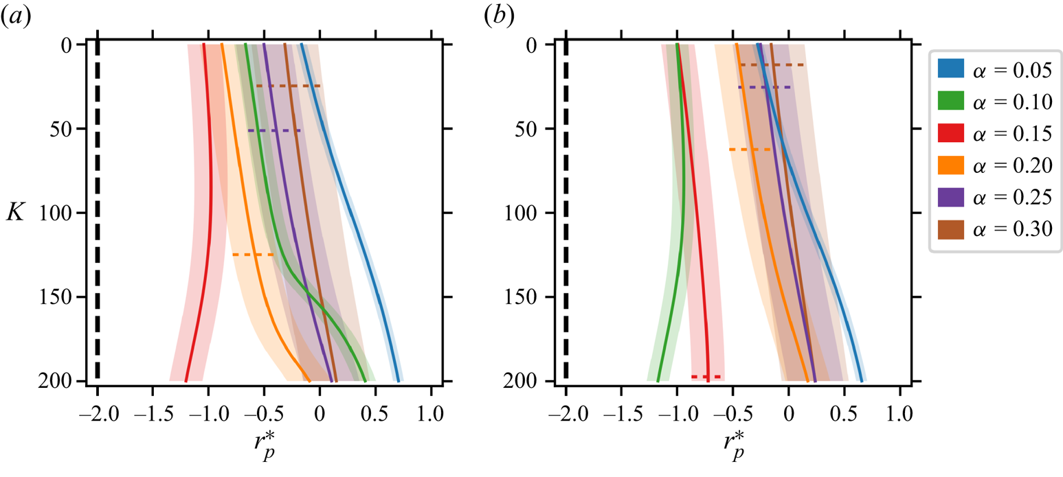
Figure 5. Lateral particle focusing as a function of the Dean number  $K$ for a cross-section with aspect ratio $2$ and bend radii (a) $\epsilon ^{-1}=80$ and (b) $\epsilon ^{-1}=160$. The horizontal focusing location, $r_{p}^{\ast }$, is non-dimensionalised with respect to $\ell /2$. Six particles are shown with radius indicated by the shading around the solid line denoting the location of the stable equilibrium. Note the horizontal axis has been restricted to $[-2,1]$ (from $[-2,2]$). For the larger particle sizes, a horizontal dashed line shows where $\textit {Re}_p=1$.
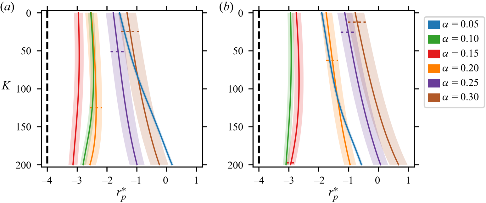
Figure 6. Lateral particle focusing as a function of the Dean number  $K$ for a cross-section with aspect ratio $4$ and bend radii (a) $\epsilon ^{-1}=80$ and (b) $\epsilon ^{-1}=160$. The horizontal focusing location, $r_{p}^{\ast }$, is non-dimensionalised with respect to $\ell /2$. Six particles are shown with radius indicated by the shading around the solid line denoting the location of the stable equilibria (for $\alpha =0.05$ this is barely perceptible). Note the horizontal axis has been restricted to $[-4,1]$ (from $[-4,4]$). For the larger particle sizes, a horizontal dashed line shows where $\textit {Re}_p=1$.
First, we consider a duct with aspect ratio  $2$ and dimensionless bend radius $\epsilon ^{-1}=80$. Figure 5(a) illustrates a small degree of separation of the different particle sizes when $K=0$ (interpreted as the behaviour in the limit $K\to 0$ as a result of a decaying flow rate). As $K$ increases, the particles with $\alpha =0.05,0.15$ become increasingly separated from the others. The stable equilibrium pair for $\alpha =0.15$ initially has $r_p^\ast \approx -1$, and initially shifts slightly towards the centre as $K$ increases before swinging back towards the left/inside wall. The stable equilibrium pair for $\alpha =0.05$ begins with $r\approx -0.16$ and steadily shifts towards the right (outside wall), up to $r\approx 0.67$. In contrast, the remaining particle sizes begin with centre between the other two and shift towards slightly right of centre without spreading significantly. Interestingly, the $\alpha =0.10$ particle experiences a relatively rapid shift toward the outside wall around $K=150$, enough to give it some small separation from the $\alpha =0.20$ particle. The relative ordering between the neighbouring particle sizes at small flow rates is explained by the approximate collapse of focusing location when plotted against $\kappa =\ell ^4/(4a^3R)$ (Harding et al. Reference Harding, Stokes and Bertozzi2019). This ordering remains consistent over the range of $K$ considered and is explored further in § 5.4.
Figure 5(b) illustrates the case with the larger bend radius  $\epsilon ^{-1}=160$. The $\alpha =0.10,0.15$ particles begin separated from the others when $K=0$. As $K$ increases, so does the separation between the two groups. Moreover, the $\alpha =0.10$ particle becomes slightly separated from that with $\alpha =0.15$ for $K>150$ as it shifts towards the inside wall, similar to the $\epsilon ^{-1}=80$ case, the $\alpha =0.05$ particle becomes slightly separated from the other group as it more rapidly shifts towards the outside wall. From a practical perspective it is useful that the clear separation between the initial two groups of particles is maintained for increasing $K$ in this particular case.
We now examine the results for a duct with aspect ratio  $4$ shown in figure 6. With $\epsilon ^{-1}=80$, the $\alpha =0.10,0.15,0.20$ particles are closer to the inside wall than the others at $K=0$. This separation increases for increasing $K$, largely due to $r_p^\ast$ for those $\alpha =0.05,0.25,0.30$ particles shifting towards the outside wall. Additionally, each of the $\alpha =0.05,0.25,0.30$ particles attains a small degree of separation from each other for $K$ approaching $200$. The $\alpha =0.15$ particle also achieves some separation from the $\alpha =0.10,0.20$ particles over the entire range of $K$, with maximum separation when $K\approx 125$. For $\alpha =0.05$, as $K$ approaches $200$ there is a bifurcation that leads to a second pair of stable equilibria in the half of the duct nearer to the outside wall. This is not evident in the figure as we have truncated the horizontal axis to $r=1$ to provide a clearer view of the region where most particles focus. A discussion surrounding this second pair of stable equilibria is deferred to § 5.2.
With  $\epsilon ^{-1}=160$, there are three distinct groups when $K=0$, namely $\alpha =0.10,0.15$, $\alpha =0.05,0.20$ and $\alpha =0.25,0.30$ ordered from the inside wall to the outside wall. The separation between the three groups is maintained for increasing $K$, with the first group becoming increasingly separated from the latter two.
All together, these results suggest several significant trends. First, clear separation between the stable equilibria of groups of different particle sizes at a low flow rate is not adversely affected as the Dean number increases. Second, particle sizes which focus near the left wall when  $K=0$ do not move significantly for increasing $K$ and, as a consequence, become increasingly separated from the other particle sizes which shift towards the outside wall. Third, the $\alpha =0.05$ particle tends to focus near the larger particles but can achieve some separation for large enough $K$. The $\alpha =0.15$ particle appears to be well separated from the remainder of the particles most consistently across these results.
5.2. Trajectory illustrations
We provide illustrations of particle trajectories towards stable equilibria for some selected values of  $\alpha,\epsilon ^{-1},K$. It should be emphasised that our model does not necessarily provide an accurate approximation of trajectories away from equilibria due to the neglect of acceleration effects. However, they do help to illustrate several things. First, if a particle were momentarily held in a specific location within the cross section (while still travelling down the main axis at some equilibrium velocity and spin), our illustrations show the direction it would go when released. Second, we see where unstable and saddle equilibria are located relative to the stable focusing positions. Third, in many cases we observe heteroclinic orbits joining a saddle equilibrium and a stable equilibrium onto which particles are initially attracted. Often, the heteroclinic orbit constitutes a slow manifold and the migration along the orbit may be sufficiently slow that the neglect of acceleration effects in our model is reasonable. Consequently these heteroclinic orbits are likely to be reasonably accurate trajectories. Put together, these observations help to elucidate the effect of increasing Dean number on the migration dynamics of particles and assist with the interpretation of the results from § 5.1.
Figure 7 illustrates trajectories of two distinct particle sizes at three different Dean numbers in a curved duct with aspect ratio 2 and dimensionless bend radius  $\epsilon ^{-1}=80$. The stable equilibrium pair for the $\alpha =0.10$ particle shifts to the right as $K$ increases (as also evident in figure 5a) and the trajectories deform accordingly. Conversely, the equilibrium pair of the slightly larger $\alpha =0.15$ particle shifts very little over this range of $K$. For increasing $K$, particles starting near the inside (left) wall migrate further to the right before making their way back to a stable equilibrium along the slow manifold. Additionally, when $K=200$ we observe a slight deformation of the slow manifold, evident as a pinch near its centre. Observe that the horizontal location of the stable equilibrium pair for the two particle sizes has only a small degree of separation when $K=1$ (compare 7(a) and 7(d)) but increases with increasing $K$ (compare 7(c) and 7( f)).
Figure 7. Trajectories of particles towards stable equilibria in a curved rectangular duct with aspect ratio  $2$ and dimensionless bend radius $\epsilon ^{-1}=80$. The particle has size (a–c) $\alpha =0.10$ and (d–f) $\alpha =0.15$, and the Dean number has values (a,d) $K=1$, (b,e) $K=100$ and (c, f) $K=200$. The left side is the inside wall of the curved duct. Stable equilibria are green, saddle equilibria are yellow and unstable equilibria are red. The marker size reflects the size of the particle.
Figure 8 similarly illustrates trajectories of two distinct particle sizes at three different Dean numbers in a curved duct with aspect ratio 2, but with the dimensionless bend radius  $\epsilon ^{-1}=160$. The stable equilibrium pair for the $\alpha =0.10$ particle does not shift much as $K$ increases (as also evident in figure 5b), but particles starting near the inside (left) wall migrate further to the right before making their way back to a stable equilibrium along the slow manifold. Additionally, when $K=200$ we again observe a slight pinching deformation of the slow manifold. This is much like the behaviour when $\alpha =0.15$ and $\epsilon ^{-1}=80$ from figure 7. For the larger $\alpha =0.20$ particle, the stable equilibrium pair shifts to the right with increasing $K$ but with only subtle changes to the trajectories as a whole. Again we observe that the horizontal separation of stable equilibria between the two particle sizes increases with increasing $K$, however, in this case, it is the larger particle that shifts towards the outer wall, unlike the case in figure 7.
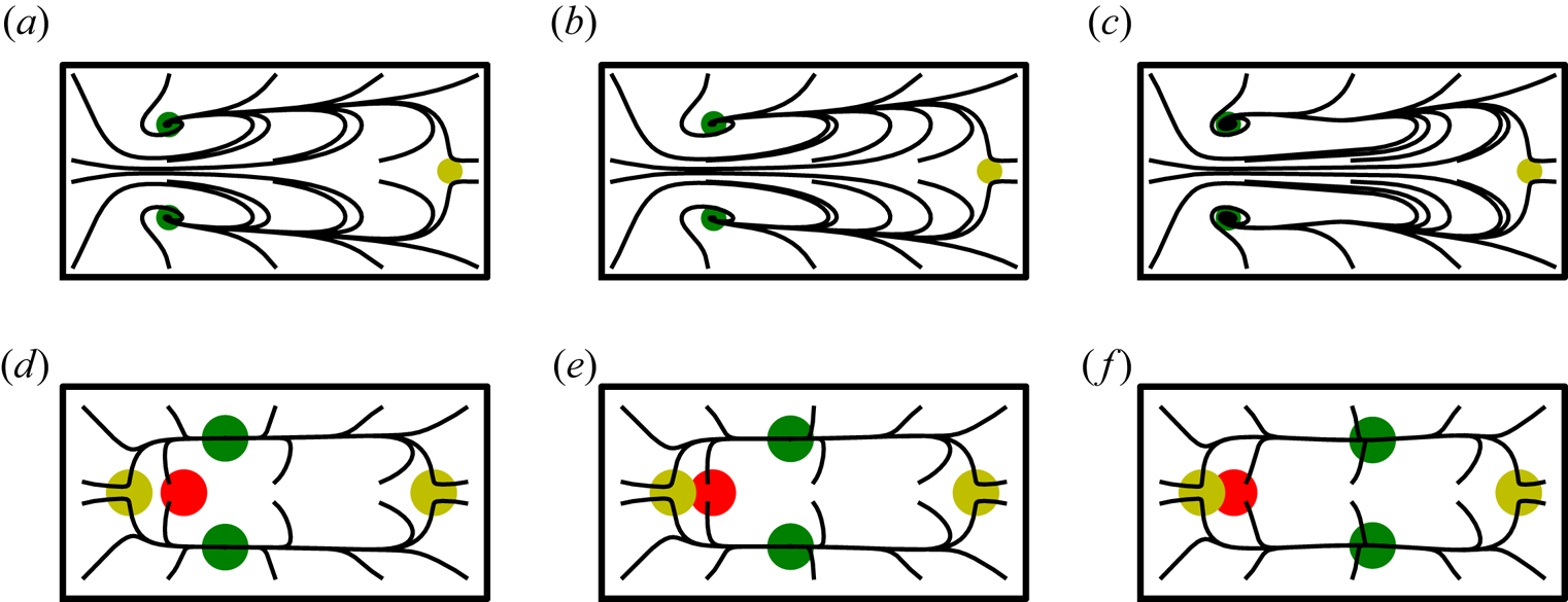
Figure 8. Trajectories of particles towards stable equilibria in a curved rectangular duct with aspect ratio  $2$ and dimensionless bend radius $\epsilon ^{-1}=160$. The particles have sizes (a–c) $\alpha =0.10$ and (d–f) $\alpha =0.20$, and the Dean number has values (a,d) $K=1$, (b,e) $K=100$ and (c, f) $K=200$. The left side is the inside wall of the curved duct. Stable equilibria are green, saddle equilibria are yellow and unstable equilibria are red. The marker size reflects the size of the particle.
Figure 9 illustrates trajectories of two distinct particle sizes at three different Dean numbers in a curved duct with aspect ratio  $4$ and dimensionless bend radius $\epsilon ^{-1}=80$. For the larger $\alpha =0.20$ particle there is almost no perceptible change in the migration dynamics over this range of $K$ values. In contrast, the stable equilibrium pair for the smaller $\alpha =0.05$ particle shifts to the right with increasing $K$ and the spiral trajectories become increasingly elongated. For $K=200$ there is an additional pair of stable equilibria located nearer to the outer wall and, although not easily seen in the figure, this pair captures more of the particles than the stable pair located closer to the centre. It is unclear if this would be observed in practice for several reasons. The first is that small particles generally do not have sufficient time/distance to fully focus, e.g. as is often evident by wide bands in fluorescent streak images (Rafeie et al. Reference Rafeie, Hosseinzadeh, Taylor and Warkiani2019). Another is that some degree of pre-focusing within the inlet regions may pre-select one of the equilibrium pairs, e.g. as is suspected to occur with straight rectangular ducts in which small particles have a stable equilibrium near the sidewalls which is rarely observed (Harding et al. Reference Harding, Stokes and Bertozzi2019). Lastly, at $K=200$ our background flow model is near the limit of its applicability where the accuracy is $O(10)\%$, so we cannot rule out this second pair being a model error.
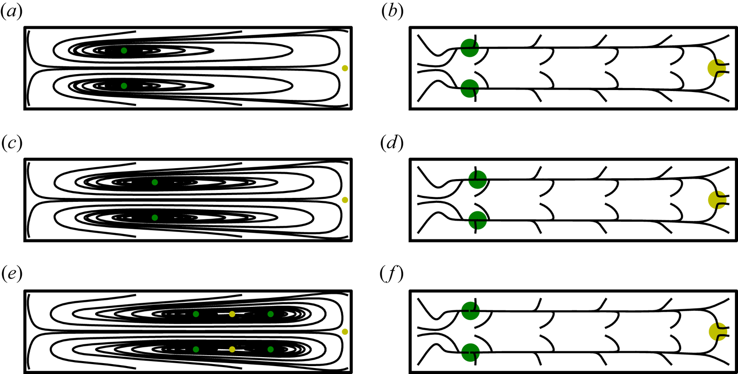
Figure 9. Trajectories of particles towards stable equilibria in a curved rectangular duct with aspect ratio  $2$ and dimensionless bend radius $\epsilon ^{-1}=80$. The particle size is (a,c,e) $\alpha =0.05$ and (b,d, f) $\alpha =0.20$, and the Dean number has values (a,b) $K=1$, (c,d) $K=100$ and (e, f) $K=200$. The left side is the inside wall of the curved duct. Stable equilibria are green, saddle equilibria are yellow and unstable equilibria are red. The marker size reflects the size of the particle.
Figure 10 illustrates trajectories of two distinct particle sizes at three different Dean numbers in a curved duct with aspect ratio 4, but with dimensionless bend radius  $\epsilon ^{-1}=160$. We observe the dynamics of the smaller $\alpha =0.10$ particle changes very little over this range of $K$. The stable equilibrium pair for the larger $\alpha =0.20$ particle shifts towards the centre along the slow manifold for increasing $K$ but with almost no perceptible change in the dynamics of trajectories otherwise. Note that the horizontal separation between the larger and smaller particle again increases with $K$.
$K$.
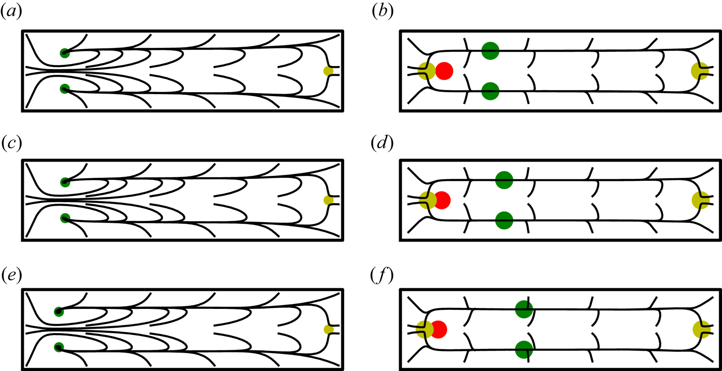
Figure 10. Trajectories of particles towards stable equilibria in a curved rectangular duct with aspect ratio  $2$ and dimensionless bend radius $\epsilon ^{-1}=160$. The particle size is (a,c,e) $\alpha =0.10$ and (b,d, f) $\alpha =0.20$, and the Dean number has values (a,b) $K=1$, (c,d) $K=100$ and (e, f) $K=200$. The left side is the inside wall of the curved duct. Stable equilibria are green, saddle equilibria are yellow and unstable equilibria are red. The marker size reflects the size of the particle.
5.3. Comparison with an experimental study
Rafeie et al. (Reference Rafeie, Hosseinzadeh, Taylor and Warkiani2019) studied particle focusing in a spiral duct with rectangular cross-section having aspect ratio  $4$ (designated design R3). For backward flow (going from the innermost to the outermost turn) $\epsilon ^{-1}\approx 180$ near the outlet, while for forward flow (from the outermost to the innermost turn) $\epsilon ^{-1}\approx 74$ near the outlet. These two values are reasonably close to the two values $\epsilon ^{-1}=160,80$ presented in our study. They experimented with three particle sizes $\alpha \approx 0.04,0.067,0.1$ and used flow rates from $0.5$ to $9.0$ ml min $^{-1}$ in steps of $0.5$ ml min $^{-1}$ (corresponding to Dean numbers from $K\approx 2$ up to $840$ at the innermost turn). Their results suggest the smallest particle remains unfocused for both flow directions, and appears to be distributed more uniformly for larger flow rates. On the other hand, the larger two particle sizes start focused near the inside wall at low flow rates and shift significantly towards the outside wall as the flow rate increases.
Bearing in mind that  $K=200$ only covers up to a flow rate of approximately $5.0$ ml min $^{-1}$ for this specific device (with $K$ measured on the innermost turn), we observe that the shifting of the two larger particle sizes towards the outside wall is qualitatively similar behaviour to our predictions for a $\alpha =0.05$ particle. Curiously, our $\alpha =0.10$ results suggest this particle stays near the inside wall, something that is not observed in the experiments for this particle size. In the case of the smaller particles in the experiment ( $\alpha \approx 0.04$ and $\alpha \approx 0.067$) the wide spread of streaks suggests the particle has had insufficient time/distance to fully focus. In § 5.2, and specifically figure 10(c), our model suggests that particles will slowly spiral in towards a stable equilibrium, which is consistent with the wide streaks observed prior to focusing being achieved. It is also evident that any small perturbations vertically away from the stable equilibrium will force the particle back onto a wide spiral path. Thus, these stable equilibria might be particularly difficult to observe in the presence of experimental noise. We must also consider that our model may not accurately predict trajectories in these specific cases due to the neglect of acceleration effects.
5.4. Approximate collapse of horizontal focusing location
In Harding et al. (Reference Harding, Stokes and Bertozzi2019) it was demonstrated that at low flow rates the horizontal location of stable equilibrium pairs approximately collapses when plotted against  $\kappa$. The local minimum in this curve helps to explain the specific focusing order of different size particles within the cross-section. Here we investigate whether this remains the case when the Dean number increases.
In figure 11 we plot the horizontal focusing location of stable equilibria, denoted  $\tilde {r}_{p}^{\ast }$, for the three Dean numbers $K=50,100,150$ in the case of a duct cross-section with aspect ratio $2$. To facilitate comparison between different particle sizes, here, $\tilde {r}_p^\ast$ has been non-dimensionalised with respect to half of the duct height. Panels (a,c,e) show the change in $r_{p}^{\ast }$ vs $\epsilon ^{-1}$ which is of practical interest when different size particles are suspended in flow through a duct having a specific bend radius. Panels (b,d,f) show the change in $r_{p}^{\ast }$ vs $\kappa$ and illustrates how this parameter characterises the focusing behaviour.
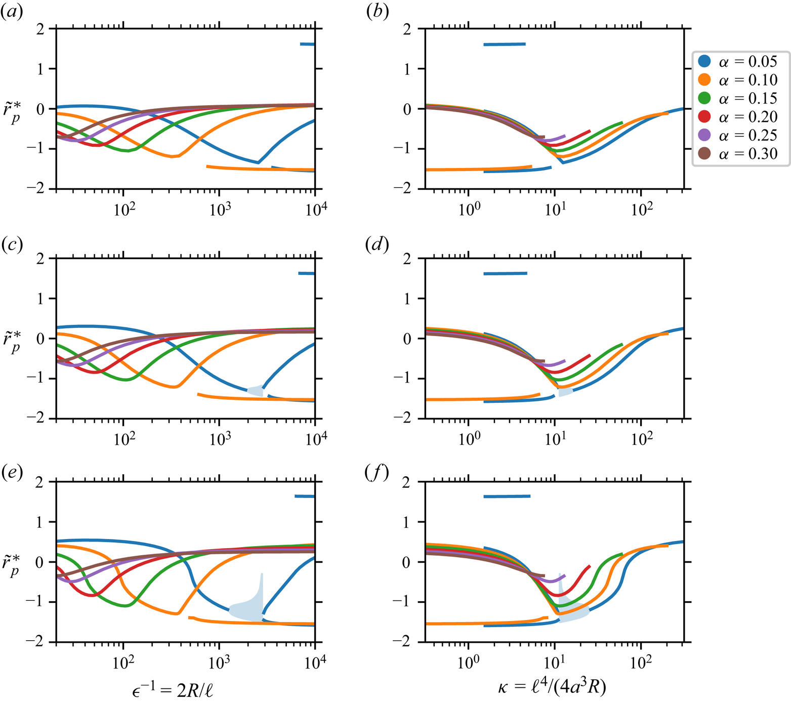
Figure 11. Horizontal location of stable equilibria  $\tilde {r}_{p}^{\ast }$ vs (a,c,e) $\epsilon ^{-1}$ and (b,d,e) $\kappa$, for the Dean numbers (a,b) $K=50$, (c,d) $K=100$ and (e, f) $K=150$. The duct cross-section has aspect ratio $2$ and $\tilde {r}_{p}^{\ast }$ is non-dimensionalised with respect to $\ell /2$. The light shaded area illustrates the region occupied by a stable orbit which occurs only when $\alpha =0.05$ for $K\gtrsim 100$.
Panels (a,b) illustrate the case  $K=50$ which is similar to the low flow rate results of Harding et al. (Reference Harding, Stokes and Bertozzi2019), with just a slight shift towards the outside wall ( $\tilde {r}=2$) of stable equilibria which focus near the centre ( $\tilde {r}=0$). We also include two additional particle sizes $\alpha =0.25,0.30$ here. Panels (c,d) show the case of $K=100$ and, qualitatively, the results are very similar. The main difference is that the increased flow rate shifts stable equilibria located near the centre (most noticeably those with $|\tilde {r}|\leq 1/2$) further towards the outside wall ( $\tilde {r}=2$). Additionally, for a narrow range of $\epsilon ^{-1}$, we observe that $\alpha =0.05$ particles no longer focus to stable equilibria but, instead, onto small stable orbits around unstable equilibria. Panels (e,f) show the case of $K=150$. A more pronounced shift in centrally focused equilibria is seen and there are subtle qualitative changes, particularly in relation to how sharply $\tilde {r}_p^\ast$ changes for larger $\kappa$ values. Additionally, the stable orbits that occur for the particle size $\alpha =0.05$ now exist over a larger range of $\epsilon ^{-1}$ and cover a larger portion of the cross-section.
The approximate collapse of focusing behaviour against  $\kappa$ is preserved remarkably well as the Dean number $K$ is increased to a moderate size. This result is significant in that it indicates that sized based separation of particles via inertial focusing should be reasonably robust to changes in flow rate. Moreover we observe that particles focused closer to the centre of the duct shift towards the outer wall as the flow rate increases whereas those that are focused closer to the inside wall do not move quite so much. This results in a slightly deeper trough in the plots of $r_{p}^{\ast }$ against $\kappa$ and further supports the previous observation that separation is typically improved with increased flow rate.
As discussed in Harding et al. (Reference Harding, Stokes and Bertozzi2019), the tail of data points where  $\alpha =0.05$ and $\kappa <10$ is due to stable equilibria appearing near the centre of the inside and outside walls. These occur for large $\epsilon ^{-1}$ as the duct becomes straighter and secondary flow drag becomes negligible in comparison with the inertial lift force such that the equilibria of a straight rectangular duct are attained. Similar stable equilibria near the centre of the inside wall exist for $\alpha =0.10$ and $\kappa <10$, although we expect these to ultimately disappear again in the limit $\kappa \to 0$ (as a straight duct has no such equilibria). The basin of attraction of these particular equilibria is very small and so it is reasonable to ignore them from a practical viewpoint (although they were included here for completeness).
We briefly remark on the existence of stable orbits when  $\alpha =0.05$ for sufficiently large $K$. For these parameters there are no stable equilibria but instead a vertically symmetric pair of unstable (spiral) equilibria and around each of these there is a reasonably tight stable orbit. These stable orbits occur over a relatively small parameter space for rectangular ducts in comparison with the case of square ducts whose dynamics is studied in Ha et al. (Reference Ha, Harding, Bertozzi and Stokes2022). In this instance the required bend radius is $O(1000)$ times the duct height which is unlikely to occur in a practical setting. Moreover, we expect that experimental noise would impact the stability of such orbits thereby making them difficult to observe experimentally.
Figure 12 shows  $r_{p}^{\ast }$ against $\epsilon ^{-1}$ and $\kappa$ for a cross-section with aspect ratio $4$ and with Dean numbers $K=50,100,150$. The main observation is that again centrally located equilibria shift closer to the outside wall with increasing $K$ which ultimately means separation can occur across a larger portion of the duct width. The approximate collapse of the focusing curves against $\kappa$ for $\kappa <10$ is incredibly well preserved as $K$ increases. The wider aspect ratio duct does not feature any stable equilibria appearing near the centre of the inside or outside wall, and stable orbits are very small where they do occur, thereby making the wider aspect ratio duct more attractive for size-based separation.
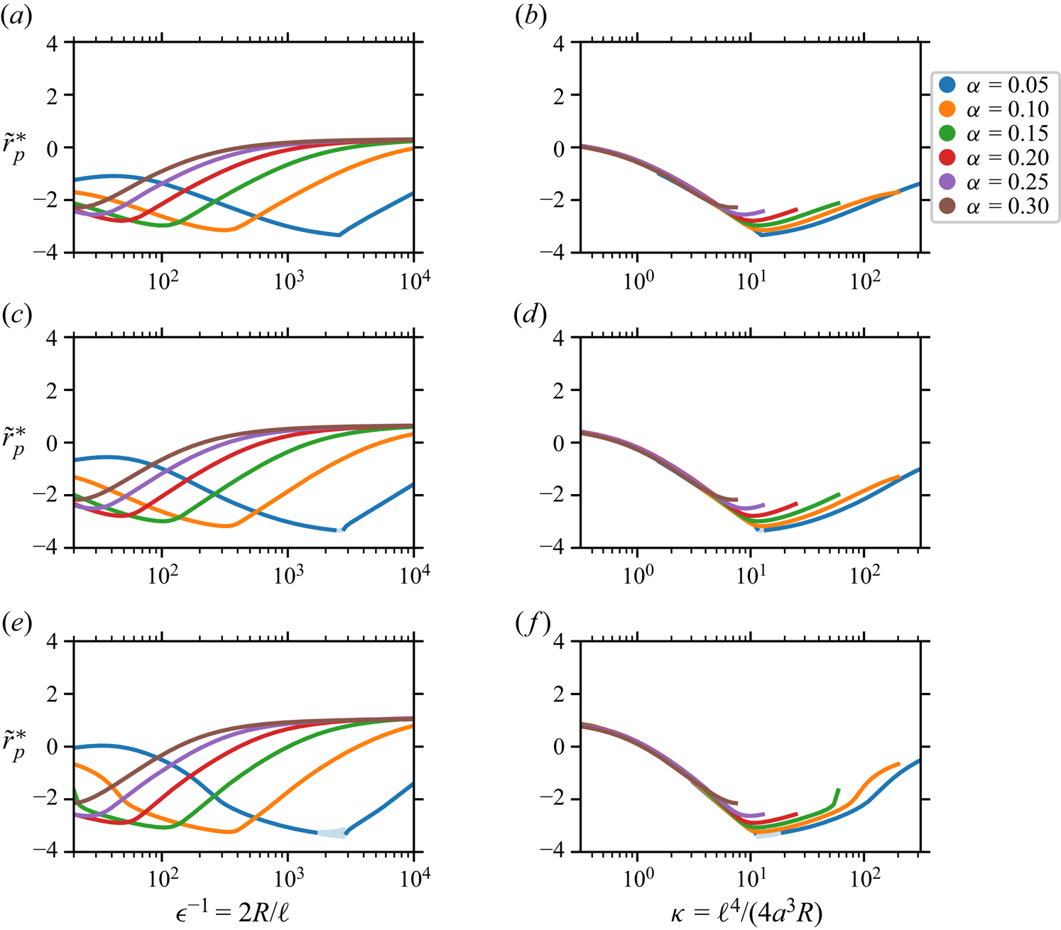
Figure 12. Horizontal location of stable equilibria  $\tilde {r}_{p}^{\ast }$ vs (a,c,e) $\epsilon ^{-1}$ and (b,d,e) $\kappa$, for the Dean numbers (a,b) $K=50$, (c,d) $K=100$ and (e, f) $K=150$. The duct cross-section has aspect ratio $4$ and $\tilde {r}_{p}^{\ast }$ is non-dimensionalised with respect to $\ell /2$. The light shaded area illustrates the region occupied by a stable orbit which occurs only when $\alpha =0.05$ for $K\gtrsim 100$.
6. Conclusions
We have extended our model of inertial migration of neutrally buoyant spherical particles in curved microfluidic ducts to moderate Dean number by incorporating further terms of a suitable perturbation approximation of the background flow. This approach is particularly powerful as the computed coefficient arrays can be cheaply re-assembled to model particle trajectories at any desired flow rate for which the model is applicable. We have demonstrated a smooth shift in stable equilibria with respect to the Dean number  $K$, up to $O(100)$, and observed that increasing $K$ can enhance the separation of particles by size. Moreover, we illustrate that the approximate collapse of the horizontal location of equilibria when plotted against $\kappa$ appears to be robust with respect to increasing $K$.
$K$.
There are, of course, some limitations to the present model. One limitation is that the model may not produce an accurate estimate of trajectories when cross-section migration is fast enough that acceleration of the particle and surrounding fluid becomes important. More research is required to determine suitable criteria to distinguish when this might be an issue, and more still to produce a model which can accurately account for acceleration related effects. Another limitation is that while we have accounted for changes in the background/Dean flow with increasing  $K$, we have not accounted for nonlinear feedback in the disturbance flow beyond the first-order terms. It is presently unknown up to what $\textit {Re}_p$ the regular perturbation expansion of the disturbance flow remains valid. One way to estimate this might be via direct comparisons with the full solution of the Navier–Stokes equation (2.3) over suitable samples of the parameter space. Investigating precisely when the regular perturbation fails and finding a suitable alternative approach for complex duct geometries remains the subject of ongoing work. Despite these limitations, our model provides, at least, some qualitative insight into how the flow rate modifies particle focusing in curved microfluidic ducts.
Non-neutrally buoyant particles could easily be incorporated into this model by adding the appropriate perturbations as described in Harding & Stokes (Reference Harding and Stokes2020). We chose to focus on neutrally buoyant particles in this work to simplify the presentation and because our previous study concluded that small variations in buoyancy have negligible effect on the particle dynamics.
A natural question going forwards is to understand how particle migration is perturbed by higher flow rates. This poses several challenges to the approach used herein. First, the regular perturbation expansion of the background flow (3.3) fails to converge for  $K$ values larger than roughly $212$ (Harding Reference Harding2019d). Thus, another suitable approximation will be required, or the background flow will need to be computed/estimated more directly. Second, $\textit {Re}_p$ cannot remain suitably small without the particle size becoming unreasonably small (taking the fluid properties to be fixed). Therefore, either additional terms in the perturbation expansion of the disturbance flow may need to be incorporated, or else a singular perturbation may be required. In either case, this significantly changes how one can implement the model and poses new computational challenges. As mentioned above, this might also have some relevance to the moderate Dean numbers considered herein. Third, it may no longer be appropriate to neglect the effects of particle acceleration, particularly if one is interested in modelling complete particle trajectories. Each of these challenges will be considered going forwards as we continue to expand and improve the modelling of inertial migration in curved ducts.
Funding
This research is supported under the Australian Research Council's Discovery Projects funding scheme (DP200100834) and a Future Fellowship (FT160100108) to Y.M.S. High performance computing resources provided by the Rāpoi HPC Cluster at Victoria University of Wellington and the Phoenix HPC service at the University of Adelaide were employed.
Declaration of interests
The authors report no conflicts of interest.
Appendix A. Application of the reciprocal theorem to calculating hydrodynamic force and torque
For completeness we begin by recalling the Lorentz reciprocal theorem for Stokes flow in its most general form and then revisit its application to the calculation of the force on a portion of the boundary of the fluid domain. Following this we illustrate how it can also be applied to the calculation of the torque about a desired reference point over a portion of the boundary of the fluid domain.
Theorem Let  $p,\boldsymbol {u}$ and $q,\boldsymbol {v}$ be the solution of
 $$\begin{gather} \boldsymbol{\nabla}\boldsymbol{\cdot} \left({-}p{\mathsf{I}}+\mu\left(\boldsymbol{\nabla}\boldsymbol{u}+ \boldsymbol{\nabla}\boldsymbol{u}^{\intercal}\right)\right) = \boldsymbol{f},\quad \boldsymbol{\nabla}\boldsymbol{\cdot} \left({-}q{\mathsf{I}}+\mu\left(\boldsymbol{\nabla}\boldsymbol{v}+ \boldsymbol{\nabla}\boldsymbol{v}^{\intercal}\right)\right) = \boldsymbol{g} \quad \text{in}\ \varOmega, \end{gather}$$
 $$\begin{gather}\boldsymbol{\nabla}\boldsymbol{\cdot}\boldsymbol{u} = 0,\quad \boldsymbol{\nabla}\boldsymbol{\cdot}\boldsymbol{v} = 0 \quad \text{in}\ \varOmega, \end{gather}$$
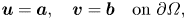 $$\begin{gather}\boldsymbol{u} = \boldsymbol{a},\quad \boldsymbol{v} = \boldsymbol{b} \quad \text{on}\ \partial\varOmega, \end{gather}$$
where  $\boldsymbol {a},\boldsymbol {b},\boldsymbol {f},\boldsymbol {g}$ are suitably smooth vector fields over their respective domains, then
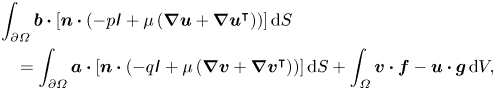 \begin{align} & \int_{\partial\varOmega}\boldsymbol{b}\boldsymbol{\cdot} \left[\boldsymbol{n}\boldsymbol{\cdot}\left({-}p{\mathsf{I}}+ \mu\left(\boldsymbol{\nabla}\boldsymbol{u}+\boldsymbol{\nabla}\boldsymbol{u}^{\intercal}\right)\right)\right]{\rm d}S \nonumber\\ &\quad =\int_{\partial\varOmega}\boldsymbol{a}\boldsymbol{\cdot} \left[\boldsymbol{n}\boldsymbol{\cdot}\left({-}q{\mathsf{I}}+\mu \left(\boldsymbol{\nabla}\boldsymbol{v}+\boldsymbol{\nabla}\boldsymbol{v}^{\intercal}\right)\right)\right]{\rm d}S + \int_{\varOmega}\boldsymbol{v}\boldsymbol{\cdot}\boldsymbol{f}-\boldsymbol{u} \boldsymbol{\cdot}\boldsymbol{g}\,{\rm d}V, \end{align}
where  $\boldsymbol {n}$ denotes the outward pointing normal vector with respect to $\varOmega$.
Proof. Observe that (A1) implies that
 $$\begin{gather} \boldsymbol{v}\boldsymbol{\cdot}\left[\boldsymbol{\nabla}\boldsymbol{\cdot} \left({-}p{\mathsf{I}}+\mu\left(\boldsymbol{\nabla}\boldsymbol{u}+\boldsymbol{\nabla}\boldsymbol{u}^{\intercal}\right)\right)-\boldsymbol{f}\right]=0, \end{gather}$$
 $$\begin{gather}\boldsymbol{u}\boldsymbol{\cdot}\left[\boldsymbol{\nabla}\boldsymbol{\cdot} \left({-}q{\mathsf{I}}+\mu\left(\boldsymbol{\nabla}\boldsymbol{v}+\boldsymbol{\nabla}\boldsymbol{v}^{\intercal}\right)\right)-\boldsymbol{g}\right]=0, \end{gather}$$
over  $\varOmega$. In general, given a differentiable tensor field ${\mathsf{S}}$, one has $\boldsymbol {\nabla }\boldsymbol {\cdot }(\boldsymbol {v}\boldsymbol {\cdot } {\mathsf{S}})=\boldsymbol {v}\boldsymbol {\cdot } (\boldsymbol {\nabla }\boldsymbol {\cdot }{\mathsf{S}})+ \boldsymbol {\nabla }\boldsymbol {v}:{\mathsf{S}}$ where $:$ is the tensor double dot product. Therefore (A3) can be written as
 $$\begin{gather} \boldsymbol{\nabla}\boldsymbol{\cdot}\left[\boldsymbol{v}\boldsymbol{\cdot} \left({-}p{\mathsf{I}}+\mu\left(\boldsymbol{\nabla}\boldsymbol{u}+\boldsymbol{\nabla} \boldsymbol{u}^{\intercal}\right)\right)\right]-\boldsymbol{\nabla}\boldsymbol{v}: \left({-}p{\mathsf{I}}+\mu\left(\boldsymbol{\nabla}\boldsymbol{u}+\boldsymbol{\nabla} \boldsymbol{u}^{\intercal}\right)\right)=\boldsymbol{v}\boldsymbol{\cdot}\boldsymbol{f}, \end{gather}$$
 $$\begin{gather}\boldsymbol{\nabla}\boldsymbol{\cdot}\left[\boldsymbol{u}\boldsymbol{\cdot} \left({-}q{\mathsf{I}}+\mu\left(\boldsymbol{\nabla}\boldsymbol{v}+\boldsymbol{\nabla} \boldsymbol{v}^{\intercal}\right)\right)\right]-\boldsymbol{\nabla}\boldsymbol{u}: \left({-}q{\mathsf{I}}+\mu\left(\boldsymbol{\nabla}\boldsymbol{v}+\boldsymbol{\nabla} \boldsymbol{v}^{\intercal}\right)\right)=\boldsymbol{u}\boldsymbol{\cdot}\boldsymbol{g}. \end{gather}$$
Subtracting the second equation from the first, then noting  $\boldsymbol {\nabla }\boldsymbol {v}: p{\mathsf{I}}=p(\boldsymbol {\nabla }\boldsymbol {\cdot }\boldsymbol {v})=0$ and $\boldsymbol {\nabla }\boldsymbol {u}: q{\mathsf{I}}=q(\boldsymbol {\nabla }\boldsymbol {\cdot }\boldsymbol {u})=0$, and additionally $\boldsymbol {\nabla }\boldsymbol {u}:\boldsymbol {\nabla }\boldsymbol {v}= \boldsymbol {\nabla }\boldsymbol {v}:\boldsymbol {\nabla }\boldsymbol {u}$ and $\boldsymbol {\nabla }\boldsymbol {u}:\boldsymbol {\nabla }\boldsymbol {v}^{\intercal }= \boldsymbol {\nabla }\boldsymbol {u}^{\intercal }: \boldsymbol {\nabla }\boldsymbol {v}=\boldsymbol {\nabla }\boldsymbol {v}: \boldsymbol {\nabla }\boldsymbol {u}^{\intercal }$, then
 \begin{align} \boldsymbol{\nabla}\boldsymbol{\cdot}\left[\boldsymbol{v}\boldsymbol{\cdot} \left({-}p{\mathsf{I}}+\mu\left(\boldsymbol{\nabla}\boldsymbol{u}+\boldsymbol{\nabla}\boldsymbol{u}^{\intercal}\right)\right)\right] -\boldsymbol{\nabla}\boldsymbol{\cdot}\left[\boldsymbol{u}\boldsymbol{\cdot} \left({-}q{\mathsf{I}}+\mu\left(\boldsymbol{\nabla}\boldsymbol{v}+\boldsymbol{\nabla}\boldsymbol{v}^{\intercal}\right)\right)\right] =\boldsymbol{v}\boldsymbol{\cdot}\boldsymbol{f}-\boldsymbol{u}\boldsymbol{\cdot}\boldsymbol{g}. \end{align}
It remains to integrate this equation over  $\varOmega$ and apply the divergence theorem to the left hand side. The result is then straightforward to re-arrange to obtain (A2).
Now we consider the reciprocal theorem applied to the calculation of the hydrodynamic force from a flow  $p,\boldsymbol {u}$ on a subset of $\partial \varOmega$, e.g. denoting the surface of a particle. In particular, we consider calculating the component of the force
 \begin{equation} \int_{\varGamma}(-\boldsymbol{n})\boldsymbol{\cdot} \left({-}p{\mathsf{I}}+\mu\left(\boldsymbol{\nabla}\boldsymbol{u}+\boldsymbol{\nabla} \boldsymbol{u}^{\intercal}\right)\right){\rm d}S, \end{equation}
on the surface  $\varGamma \subset \partial \varOmega$ in the direction of a constant unit vector $\boldsymbol {e}_{\ast }$.
Corollary Let  $p,\boldsymbol {u}$ and $q,\boldsymbol {v}$ satisfy (A1) with $\boldsymbol {a}=\boldsymbol {0}$ over $\partial \varOmega$, $\boldsymbol {g}=\boldsymbol {0}$ over $\varOmega$, $\boldsymbol {b}=\boldsymbol {e}_{\ast }$ is a constant vector on $\varGamma \subset \partial \varOmega$ and $\boldsymbol {b}=\boldsymbol {0}$ over the remainder of $\partial \varOmega \backslash \varGamma$. Then
 \begin{equation} \boldsymbol{e}_{{\ast}}\boldsymbol{\cdot} \int_{\varGamma}(-\boldsymbol{n})\boldsymbol{\cdot} \left({-}p{\mathsf{I}}+\mu\left(\boldsymbol{\nabla}\boldsymbol{u}+\boldsymbol{\nabla} \boldsymbol{u}^{\intercal}\right)\right){\rm d}S ={-}\int_{\varOmega}\boldsymbol{v} \boldsymbol{\cdot}\boldsymbol{f}\,{\rm d}V. \end{equation}
Proof. Immediately, due to  $\boldsymbol {a}=\boldsymbol {0}$ and $\boldsymbol {g}=\boldsymbol {0}$, one obtains from (A2) the result
 \begin{equation} \int_{\partial\varOmega}\boldsymbol{b}\boldsymbol{\cdot} \left[\boldsymbol{n}\boldsymbol{\cdot}\left({-}p{\mathsf{I}}+\mu\left(\boldsymbol{\nabla} \boldsymbol{u}+\boldsymbol{\nabla}\boldsymbol{u}^{\intercal}\right)\right)\right]{\rm d}S = \int_{\varOmega}\boldsymbol{v}\boldsymbol{\cdot}\boldsymbol{f}\,{\rm d}V. \end{equation}
Since  $\boldsymbol {v}=\boldsymbol {b}=\boldsymbol {e}_{\ast }$ is constant over $\varGamma$ (and is zero elsewhere) it follows that
 \begin{equation} \boldsymbol{e}_{{\ast}}\boldsymbol{\cdot}\int_{\varGamma}\boldsymbol{n} \boldsymbol{\cdot}\left({-}p{\mathsf{I}}+\mu\left(\boldsymbol{\nabla}\boldsymbol{u}+ \boldsymbol{\nabla}\boldsymbol{u}^{\intercal}\right)\right){\rm d}S = \int_{\varOmega} \boldsymbol{v}\boldsymbol{\cdot}\boldsymbol{f}\,{\rm d}V. \end{equation}
One simply needs to multiply both sides by  $-1$ to obtain the desired hydrodynamic force in the direction $\boldsymbol {e}_{\ast }$.
Observe that in the corollary  $\boldsymbol {v}$ could be written as $\boldsymbol {\mathcal {V}}(\boldsymbol {e}_{\ast })$ using the operator $\boldsymbol {\mathcal {V}}$ introduced in § 2.1, taking $\varGamma =\partial \hat {\mathcal {P}}'$. Now, we wish to apply the reciprocal theorem again to the calculation of the torque
 \begin{equation} \int_{\varGamma}(\boldsymbol{x}-\boldsymbol{x}_{c})\times \left[(-\boldsymbol{n})\boldsymbol{\cdot} \left({-}p{\mathsf{I}}+\mu\left(\boldsymbol{\nabla}\boldsymbol{u}+\boldsymbol{\nabla} \boldsymbol{u}^{\intercal}\right)\right)\right]{\rm d}S, \end{equation}
about a (fixed) reference point  $\boldsymbol {x}_{c}$, e.g. the centre of mass of a particle.
Corollary Let  $p,\boldsymbol {u}$ and $q,\boldsymbol {v}$ satisfy (A1) with $\boldsymbol {a}=\boldsymbol {0}$ over $\partial \varOmega$, $\boldsymbol {g}=\boldsymbol {0}$ over $\varOmega$, $\boldsymbol {b}=\boldsymbol {e}_{\ast }\times (\boldsymbol {x}-\boldsymbol {x}_{c})$ on $\varGamma \subset \partial \varOmega$ where $\boldsymbol {e}_{\ast }$ is constant, and $\boldsymbol {b}=\boldsymbol {0}$ over the remainder $\partial \varOmega \backslash \varGamma$. Then
 \begin{equation} \boldsymbol{e}_{{\ast}}\boldsymbol{\cdot}\int_{\varGamma}(\boldsymbol{x}-\boldsymbol{x}_{c}) \times\left[(-\boldsymbol{n})\boldsymbol{\cdot} \left({-}p{\mathsf{I}}+\mu\left(\boldsymbol{\nabla}\boldsymbol{u}+\boldsymbol{\nabla} \boldsymbol{u}^{\intercal}\right)\right)\right]{\rm d}S ={-}\int_{\varOmega}\boldsymbol{v}\boldsymbol{\cdot}\boldsymbol{f}\,{\rm d}V. \end{equation}
Proof. This time (A2) yields the result
 \begin{equation} \int_{\varGamma}\left(\boldsymbol{e}_{{\ast}}\times(\boldsymbol{x}-\boldsymbol{x}_{c})\right) \boldsymbol{\cdot}\left[\boldsymbol{n}\boldsymbol{\cdot} \left({-}p{\mathsf{I}}+\mu\left(\boldsymbol{\nabla}\boldsymbol{u}+\boldsymbol{\nabla} \boldsymbol{u}^{\intercal}\right)\right)\right]{\rm d}S = \int_{\varOmega}\boldsymbol{v}\boldsymbol{\cdot}\boldsymbol{f}\,{\rm d}V. \end{equation}
Applying the triple product shift rule  $(\boldsymbol {x}\times \boldsymbol {y})\boldsymbol {\cdot } \boldsymbol {z}=(\boldsymbol {y}\times \boldsymbol {z})\boldsymbol {\cdot }\boldsymbol {x}$ to the integrand on the left-hand side produces
 \begin{equation} \int_{\varGamma}\left((\boldsymbol{x}-\boldsymbol{x}_{c})\times\left[\boldsymbol{n} \boldsymbol{\cdot}\left({-}p{\mathsf{I}}+\mu\left(\boldsymbol{\nabla}\boldsymbol{u}+ \boldsymbol{\nabla}\boldsymbol{u}^{\intercal}\right)\right)\right]\right) \boldsymbol{\cdot}\boldsymbol{e}_{{\ast}}\,{\rm d}S = \int_{\varOmega}\boldsymbol{v}\boldsymbol{\cdot}\boldsymbol{f}\,{\rm d}V. \end{equation}
The dot product with  $\boldsymbol {e}_{\ast }$ can be safely pulled outside the integral (as $\boldsymbol {e}_{\ast }$ is constant). Multiplying both sides by $-1$ then yields the desired component of torque in the $\boldsymbol {e}_{\ast }$ direction, i.e. (A11).
Observe that using the operators introduced in § 2.1 we can write  $\boldsymbol {v}=\boldsymbol {\mathcal {V}}(\boldsymbol {e}_{\ast }\times (\boldsymbol {x}-\boldsymbol {x}_{c}))$ within this corollary, taking $\varGamma =\partial \hat {\mathcal {P}}'$.
Appendix B. Symmetries associated with Stokes flow around a spherical particle in a curved duct
Here, we describe a variety of quantities which are zero due to symmetries associated with our problem. Specifically, in the rotating frame the fluid domain  $\mathcal {F}'$ is symmetric about $\theta '=0$ and many fields of interest relating to solutions of (2.13) are either odd or even with respect to $\theta '$. Specifically, the following are odd with respect to $\theta '$:
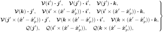 \begin{equation} \left.\begin{gathered} \boldsymbol{\mathcal{V}}(\boldsymbol{i}')\boldsymbol{\cdot}\boldsymbol{j}',\quad \boldsymbol{\mathcal{V}}(\boldsymbol{j}')\boldsymbol{\cdot}\boldsymbol{i}',\quad \boldsymbol{\mathcal{V}}(\boldsymbol{j}')\boldsymbol{\cdot}\boldsymbol{k}, \\ \boldsymbol{\mathcal{V}}(\boldsymbol{k})\boldsymbol{\cdot}\boldsymbol{j}',\quad \boldsymbol{\mathcal{V}}(\boldsymbol{i}'\times(\hat{\boldsymbol{x}}'-\hat{\boldsymbol{x}}_{p}^{\prime})) \boldsymbol{\cdot}\boldsymbol{i}',\quad \boldsymbol{\mathcal{V}} (\boldsymbol{i}'\times(\hat{\boldsymbol{x}}'-\hat{\boldsymbol{x}}_{p}^{\prime}))\boldsymbol{\cdot}\boldsymbol{k}, \\ \boldsymbol{\mathcal{V}}(\boldsymbol{j}'\times(\hat{\boldsymbol{x}}'-\hat{\boldsymbol{x}}_{p}^{\prime})) \boldsymbol{\cdot}\boldsymbol{j}',\quad \boldsymbol{\mathcal{V}}(\boldsymbol{k}\times(\hat{\boldsymbol{x}}'-\hat{\boldsymbol{x}}_{p}^{\prime})) \boldsymbol{\cdot}\boldsymbol{i}',\quad \boldsymbol{\mathcal{V}} (\boldsymbol{k}\times(\hat{\boldsymbol{x}}'-\hat{\boldsymbol{x}}_{p}^{\prime}))\boldsymbol{\cdot}\boldsymbol{k}, \\ \mathcal{Q}(\boldsymbol{j}'), \quad \mathcal{Q}(\boldsymbol{i}'\times(\hat{\boldsymbol{x}}'-\hat{\boldsymbol{x}}_{p}^{\prime})),\quad \mathcal{Q}(\boldsymbol{k}\times(\hat{\boldsymbol{x}}'-\hat{\boldsymbol{x}}_{p}^{\prime})), \end{gathered}\right\} \end{equation}
while the following are even with respect to  $\theta '$:
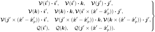 \begin{equation} \left.\begin{gathered} \boldsymbol{\mathcal{V}}(\boldsymbol{i}')\boldsymbol{\cdot}\boldsymbol{i}',\quad \boldsymbol{\mathcal{V}}(\boldsymbol{i}')\boldsymbol{\cdot}\boldsymbol{k},\quad \boldsymbol{\mathcal{V}}(\boldsymbol{j}')\boldsymbol{\cdot}\boldsymbol{j}', \\ \boldsymbol{\mathcal{V}}(\boldsymbol{k})\boldsymbol{\cdot}\boldsymbol{i}',\quad \boldsymbol{\mathcal{V}}(\boldsymbol{k})\boldsymbol{\cdot}\boldsymbol{k}, \boldsymbol{\mathcal{V}}(\boldsymbol{i}'\times(\hat{\boldsymbol{x}}'-\hat{\boldsymbol{x}}_{p}^{\prime})) \boldsymbol{\cdot}\boldsymbol{j}', \\ \boldsymbol{\mathcal{V}}(\boldsymbol{j}'\times(\hat{\boldsymbol{x}}'-\hat{\boldsymbol{x}}_{p}^{\prime})) \boldsymbol{\cdot}\boldsymbol{i}',\quad \boldsymbol{\mathcal{V}}(\boldsymbol{j}'\times(\hat{\boldsymbol{x}}'-\hat{\boldsymbol{x}}_{p}^{\prime})) \boldsymbol{\cdot}\boldsymbol{k}, \boldsymbol{\mathcal{V}}(\boldsymbol{k}\times (\hat{\boldsymbol{x}}'-\hat{\boldsymbol{x}}_{p}^{\prime}))\boldsymbol{\cdot}\boldsymbol{j}', \\ \mathcal{Q}(\boldsymbol{i}'),\quad \mathcal{Q}(\boldsymbol{k}),\quad \mathcal{Q}(\boldsymbol{j}'\times(\hat{\boldsymbol{x}}'-\hat{\boldsymbol{x}}_{p}^{\prime})). \end{gathered}\right\} \end{equation}
These parities can be used to show
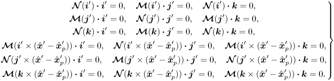 \begin{gather} \left.\begin{gathered} \boldsymbol{\mathcal{N}}(\boldsymbol{i}')\boldsymbol{\cdot}\boldsymbol{i}' = 0,\quad \boldsymbol{\mathcal{M}}(\boldsymbol{i}')\boldsymbol{\cdot}\boldsymbol{j}' = 0,\quad \boldsymbol{\mathcal{N}}(\boldsymbol{i}')\boldsymbol{\cdot}\boldsymbol{k} = 0, \\ \boldsymbol{\mathcal{M}}(\boldsymbol{j}')\boldsymbol{\cdot}\boldsymbol{i}' = 0,\quad \boldsymbol{\mathcal{N}}(\boldsymbol{j}')\boldsymbol{\cdot}\boldsymbol{j}' = 0,\quad \boldsymbol{\mathcal{M}}(\boldsymbol{j}')\boldsymbol{\cdot}\boldsymbol{k} = 0, \\ \boldsymbol{\mathcal{N}}(\boldsymbol{k})\boldsymbol{\cdot}\boldsymbol{i}' = 0,\quad \boldsymbol{\mathcal{M}}(\boldsymbol{k})\boldsymbol{\cdot}\boldsymbol{j}' = 0,\quad \boldsymbol{\mathcal{N}}(\boldsymbol{k})\boldsymbol{\cdot}\boldsymbol{k} = 0, \\ \boldsymbol{\mathcal{M}}(\boldsymbol{i}'\times(\hat{\boldsymbol{x}}'-\hat{\boldsymbol{x}}_{p}^{\prime})) \boldsymbol{\cdot}\boldsymbol{i}' = 0,\quad \boldsymbol{\mathcal{N}}(\boldsymbol{i}'\times(\hat{\boldsymbol{x}}'-\hat{\boldsymbol{x}}_{p}^{\prime})) \boldsymbol{\cdot}\boldsymbol{j}' = 0,\quad \boldsymbol{\mathcal{M}}(\boldsymbol{i}'\times(\hat{\boldsymbol{x}}'-\hat{\boldsymbol{x}}_{p}^{\prime})) \boldsymbol{\cdot}\boldsymbol{k} = 0, \\ \boldsymbol{\mathcal{N}}(\boldsymbol{j}'\times(\hat{\boldsymbol{x}}'-\hat{\boldsymbol{x}}_{p}^{\prime})) \boldsymbol{\cdot}\boldsymbol{i}' = 0,\quad \boldsymbol{\mathcal{M}}(\boldsymbol{j}'\times(\hat{\boldsymbol{x}}'-\hat{\boldsymbol{x}}_{p}^{\prime})) \boldsymbol{\cdot}\boldsymbol{j}' = 0,\quad \boldsymbol{\mathcal{N}}(\boldsymbol{j}'\times(\hat{\boldsymbol{x}}'-\hat{\boldsymbol{x}}_{p}^{\prime})) \boldsymbol{\cdot}\boldsymbol{k} = 0, \\ \boldsymbol{\mathcal{M}}(\boldsymbol{k}\times(\hat{\boldsymbol{x}}'-\hat{\boldsymbol{x}}_{p}^{\prime})) \boldsymbol{\cdot}\boldsymbol{i}' = 0,\quad \boldsymbol{\mathcal{N}}(\boldsymbol{k}\times(\hat{\boldsymbol{x}}'-\hat{\boldsymbol{x}}_{p}^{\prime})) \boldsymbol{\cdot}\boldsymbol{j}' = 0,\quad \boldsymbol{\mathcal{M}}(\boldsymbol{k}\times(\hat{\boldsymbol{x}}'-\hat{\boldsymbol{x}}_{p}^{\prime})) \boldsymbol{\cdot}\boldsymbol{k} = 0. \end{gathered}\right\} \end{gather}
Moreover, given a sufficiently smooth function  $f(r',z')$, i.e. which is independent of $\theta '$, then each of
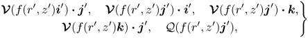 \begin{equation} \left.\begin{gathered} \boldsymbol{\mathcal{V}}(f(r',z')\boldsymbol{i}')\boldsymbol{\cdot}\boldsymbol{j}', \quad \boldsymbol{\mathcal{V}}(f(r',z')\boldsymbol{j}')\boldsymbol{\cdot}\boldsymbol{i}', \quad \boldsymbol{\mathcal{V}}(f(r',z')\boldsymbol{j}')\boldsymbol{\cdot}\boldsymbol{k}, \\ \boldsymbol{\mathcal{V}}(f(r',z')\boldsymbol{k})\boldsymbol{\cdot}\boldsymbol{j}', \quad \mathcal{Q}(f(r',z')\boldsymbol{j}'), \end{gathered}\right\} \end{equation}
are odd with respect to  $\theta '$, and each of
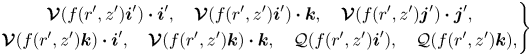 \begin{equation} \left.\begin{gathered} \boldsymbol{\mathcal{V}}(f(r',z')\boldsymbol{i}')\boldsymbol{\cdot}\boldsymbol{i}',\quad \boldsymbol{\mathcal{V}}(f(r',z')\boldsymbol{i}')\boldsymbol{\cdot}\boldsymbol{k},\quad \boldsymbol{\mathcal{V}}(f(r',z')\boldsymbol{j}')\boldsymbol{\cdot}\boldsymbol{j}', \\ \boldsymbol{\mathcal{V}}(f(r',z')\boldsymbol{k})\boldsymbol{\cdot}\boldsymbol{i}',\quad \boldsymbol{\mathcal{V}}(f(r',z')\boldsymbol{k})\boldsymbol{\cdot}\boldsymbol{k},\quad \mathcal{Q}(f(r',z')\boldsymbol{i}'),\quad \mathcal{Q}(f(r',z')\boldsymbol{k}), \end{gathered}\right\} \end{equation}
are even with respect to  $\theta '$. Consequently, one can show
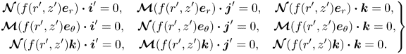 \begin{equation} \left.\begin{gathered}
\boldsymbol{\mathcal{N}}(f(r',z')\boldsymbol{e}_{r})\boldsymbol{\cdot}\boldsymbol{i}'
= 0,\quad
\boldsymbol{\mathcal{M}}(f(r',z')\boldsymbol{e}_{r})\boldsymbol{\cdot}\boldsymbol{j}'
= 0,\quad
\boldsymbol{\mathcal{N}}(f(r',z')\boldsymbol{e}_{r})\boldsymbol{\cdot}\boldsymbol{k}
= 0, \\
\boldsymbol{\mathcal{M}}(f(r',z')\boldsymbol{e}_{\theta})\boldsymbol{\cdot}\boldsymbol{i}'
= 0,\quad
\boldsymbol{\mathcal{N}}(f(r',z')\boldsymbol{e}_{\theta})\boldsymbol{\cdot}\boldsymbol{j}'
= 0,\quad
\boldsymbol{\mathcal{M}}(f(r',z')\boldsymbol{e}_{\theta})\boldsymbol{\cdot}\boldsymbol{k}
= 0, \\
\boldsymbol{\mathcal{N}}(f(r',z')\boldsymbol{k})\boldsymbol{\cdot}\boldsymbol{i}'
= 0,\quad
\boldsymbol{\mathcal{M}}(f(r',z')\boldsymbol{k})\boldsymbol{\cdot}\boldsymbol{j}'
= 0,\quad
\boldsymbol{\mathcal{N}}(f(r',z')\boldsymbol{k})\boldsymbol{\cdot}\boldsymbol{k}
= 0. \end{gathered}\right\}
\end{equation}
\begin{equation} \left.\begin{gathered}
\boldsymbol{\mathcal{N}}(f(r',z')\boldsymbol{e}_{r})\boldsymbol{\cdot}\boldsymbol{i}'
= 0,\quad
\boldsymbol{\mathcal{M}}(f(r',z')\boldsymbol{e}_{r})\boldsymbol{\cdot}\boldsymbol{j}'
= 0,\quad
\boldsymbol{\mathcal{N}}(f(r',z')\boldsymbol{e}_{r})\boldsymbol{\cdot}\boldsymbol{k}
= 0, \\
\boldsymbol{\mathcal{M}}(f(r',z')\boldsymbol{e}_{\theta})\boldsymbol{\cdot}\boldsymbol{i}'
= 0,\quad
\boldsymbol{\mathcal{N}}(f(r',z')\boldsymbol{e}_{\theta})\boldsymbol{\cdot}\boldsymbol{j}'
= 0,\quad
\boldsymbol{\mathcal{M}}(f(r',z')\boldsymbol{e}_{\theta})\boldsymbol{\cdot}\boldsymbol{k}
= 0, \\
\boldsymbol{\mathcal{N}}(f(r',z')\boldsymbol{k})\boldsymbol{\cdot}\boldsymbol{i}'
= 0,\quad
\boldsymbol{\mathcal{M}}(f(r',z')\boldsymbol{k})\boldsymbol{\cdot}\boldsymbol{j}'
= 0,\quad
\boldsymbol{\mathcal{N}}(f(r',z')\boldsymbol{k})\boldsymbol{\cdot}\boldsymbol{k}
= 0. \end{gathered}\right\}
\end{equation}
Of particular interest is when  $f(r',z')$ describes appropriate components of the background flow velocity field $\bar {\boldsymbol {u}}$, as described in § 3.
Appendix C. Further application of symmetry in the model
Similar to Harding et al. (Reference Harding, Stokes and Bertozzi2019), we can further expand  $\boldsymbol {I}_0$ to determine which terms contribute to and are most significant in (4.6) and (4.7). First, the decomposition leading to (4.2) and (4.4) suggests that $\boldsymbol {v}_{0}$ be split into two distinct parts, namely $\boldsymbol {v}_{0}=\boldsymbol {v}_{0,a}+\boldsymbol {v}_{0,s}$ where
 \begin{align} \boldsymbol{v}_{0,a} &= u_{p,0,\theta}\boldsymbol{\mathcal{V}}(\boldsymbol{j}')+ \varOmega_{p,0,r}\boldsymbol{\mathcal{V}}(\boldsymbol{i}'\times(\hat{\boldsymbol{x}}'-\hat{\boldsymbol{x}}_{p}^{\prime}))+ \varOmega_{p,0,z}\boldsymbol{\mathcal{V}}(\boldsymbol{k}\times(\hat{\boldsymbol{x}}'-\hat{\boldsymbol{x}}_{p}^{\prime})) \nonumber\\ &\quad -2\alpha^{{-}1}[\boldsymbol{\mathcal{V}}(\bar{\boldsymbol{u}}_{a,0})+K\boldsymbol{\mathcal{V}} (\bar{\boldsymbol{u}}_{a,0})+K^{2}\boldsymbol{\mathcal{V}}(\bar{\boldsymbol{u}}_{a,0})], \end{align}
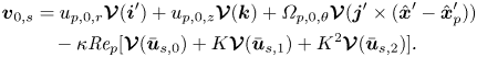 \begin{align} \boldsymbol{v}_{0,s} &= u_{p,0,r}\boldsymbol{\mathcal{V}}(\boldsymbol{i}')+u_{p,0,z} \boldsymbol{\mathcal{V}}(\boldsymbol{k})+\varOmega_{p,0,\theta}\boldsymbol{\mathcal{V}} (\boldsymbol{j}'\times(\hat{\boldsymbol{x}}'-\hat{\boldsymbol{x}}_{p}^{\prime})) \nonumber\\ &\quad -\kappa\textit{Re}_{p}[\boldsymbol{\mathcal{V}}(\bar{\boldsymbol{u}}_{s,0})+K \boldsymbol{\mathcal{V}}(\bar{\boldsymbol{u}}_{s,1})+K^{2}\boldsymbol{\mathcal{V}} (\bar{\boldsymbol{u}}_{s,2})]. \end{align}
Subsequently, we can similarly decompose  $\boldsymbol {I}_{0}$ into two distinct components, specifically $\boldsymbol {I}_{0}=\boldsymbol {I}_{0,a}+\boldsymbol {I}_{0,s}$ where
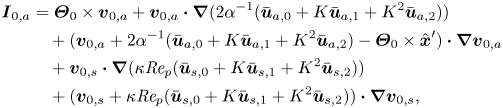 \begin{align} \boldsymbol{I}_{0,a} &=
\boldsymbol{\varTheta}_{0}\times\boldsymbol{v}_{0,a}+\boldsymbol{v}_{0,a}\boldsymbol{\cdot}
\boldsymbol{\nabla}(2\alpha^{{-}1}(\bar{\boldsymbol{u}}_{a,0}+K\bar{\boldsymbol{u}}_{a,1}+K^2\bar{\boldsymbol{u}}_{a,2}))
\nonumber\\ &\quad
+(\boldsymbol{v}_{0,a}+2\alpha^{{-}1}(\bar{\boldsymbol{u}}_{a,0}+K\bar{\boldsymbol{u}}_{a,1}+
K^2\bar{\boldsymbol{u}}_{a,2})-\boldsymbol{\varTheta}_{0}\times\hat{\boldsymbol{x}}')
\boldsymbol{\cdot}\boldsymbol{\nabla}\boldsymbol{v}_{0,a}
\nonumber\\ &\quad
+\boldsymbol{v}_{0,s}\boldsymbol{\cdot}\boldsymbol{\nabla}
(\kappa\textit{Re}_p(\bar{\boldsymbol{u}}_{s,0}+K\bar{\boldsymbol{u}}_{s,1}+K^2\bar{\boldsymbol{u}}_{s,2}))
\nonumber\\ &\quad
+(\boldsymbol{v}_{0,s}+\kappa\textit{Re}_p(\bar{\boldsymbol{u}}_{s,0}+K\bar{\boldsymbol{u}}_{s,1}+
K^2\bar{\boldsymbol{u}}_{s,2}))\boldsymbol{\cdot}\boldsymbol{\nabla}\boldsymbol{v}_{0,s},
\end{align}
\begin{align} \boldsymbol{I}_{0,a} &=
\boldsymbol{\varTheta}_{0}\times\boldsymbol{v}_{0,a}+\boldsymbol{v}_{0,a}\boldsymbol{\cdot}
\boldsymbol{\nabla}(2\alpha^{{-}1}(\bar{\boldsymbol{u}}_{a,0}+K\bar{\boldsymbol{u}}_{a,1}+K^2\bar{\boldsymbol{u}}_{a,2}))
\nonumber\\ &\quad
+(\boldsymbol{v}_{0,a}+2\alpha^{{-}1}(\bar{\boldsymbol{u}}_{a,0}+K\bar{\boldsymbol{u}}_{a,1}+
K^2\bar{\boldsymbol{u}}_{a,2})-\boldsymbol{\varTheta}_{0}\times\hat{\boldsymbol{x}}')
\boldsymbol{\cdot}\boldsymbol{\nabla}\boldsymbol{v}_{0,a}
\nonumber\\ &\quad
+\boldsymbol{v}_{0,s}\boldsymbol{\cdot}\boldsymbol{\nabla}
(\kappa\textit{Re}_p(\bar{\boldsymbol{u}}_{s,0}+K\bar{\boldsymbol{u}}_{s,1}+K^2\bar{\boldsymbol{u}}_{s,2}))
\nonumber\\ &\quad
+(\boldsymbol{v}_{0,s}+\kappa\textit{Re}_p(\bar{\boldsymbol{u}}_{s,0}+K\bar{\boldsymbol{u}}_{s,1}+
K^2\bar{\boldsymbol{u}}_{s,2}))\boldsymbol{\cdot}\boldsymbol{\nabla}\boldsymbol{v}_{0,s},
\end{align}
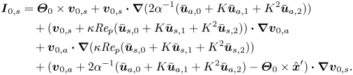 \begin{align} \boldsymbol{I}_{0,s} &=
\boldsymbol{\varTheta}_{0}\times\boldsymbol{v}_{0,s}+\boldsymbol{v}_{0,s}
\boldsymbol{\cdot}\boldsymbol{\nabla}(2\alpha^{{-}1}
(\bar{\boldsymbol{u}}_{a,0}+K\bar{\boldsymbol{u}}_{a,1}+K^2\bar{\boldsymbol{u}}_{a,2}))
\nonumber\\ &\quad
+(\boldsymbol{v}_{0,s}+\kappa\textit{Re}_p(\bar{\boldsymbol{u}}_{s,0}+K\bar{\boldsymbol{u}}_{s,1}+
K^2\bar{\boldsymbol{u}}_{s,2}))\boldsymbol{\cdot}\boldsymbol{\nabla}\boldsymbol{v}_{0,a}
\nonumber\\ &\quad
+\boldsymbol{v}_{0,a}\boldsymbol{\cdot}\boldsymbol{\nabla}
(\kappa\textit{Re}_p(\bar{\boldsymbol{u}}_{s,0}+K\bar{\boldsymbol{u}}_{s,1}+K^2\bar{\boldsymbol{u}}_{s,2}))
\nonumber\\ &\quad
+(\boldsymbol{v}_{0,a}+2\alpha^{{-}1}(\bar{\boldsymbol{u}}_{a,0}+K\bar{\boldsymbol{u}}_{a,1}+
K^2\bar{\boldsymbol{u}}_{a,2})-\boldsymbol{\varTheta}_{0}\times\hat{\boldsymbol{x}}')
\boldsymbol{\cdot}\boldsymbol{\nabla}\boldsymbol{v}_{0,s}.
\end{align}
\begin{align} \boldsymbol{I}_{0,s} &=
\boldsymbol{\varTheta}_{0}\times\boldsymbol{v}_{0,s}+\boldsymbol{v}_{0,s}
\boldsymbol{\cdot}\boldsymbol{\nabla}(2\alpha^{{-}1}
(\bar{\boldsymbol{u}}_{a,0}+K\bar{\boldsymbol{u}}_{a,1}+K^2\bar{\boldsymbol{u}}_{a,2}))
\nonumber\\ &\quad
+(\boldsymbol{v}_{0,s}+\kappa\textit{Re}_p(\bar{\boldsymbol{u}}_{s,0}+K\bar{\boldsymbol{u}}_{s,1}+
K^2\bar{\boldsymbol{u}}_{s,2}))\boldsymbol{\cdot}\boldsymbol{\nabla}\boldsymbol{v}_{0,a}
\nonumber\\ &\quad
+\boldsymbol{v}_{0,a}\boldsymbol{\cdot}\boldsymbol{\nabla}
(\kappa\textit{Re}_p(\bar{\boldsymbol{u}}_{s,0}+K\bar{\boldsymbol{u}}_{s,1}+K^2\bar{\boldsymbol{u}}_{s,2}))
\nonumber\\ &\quad
+(\boldsymbol{v}_{0,a}+2\alpha^{{-}1}(\bar{\boldsymbol{u}}_{a,0}+K\bar{\boldsymbol{u}}_{a,1}+
K^2\bar{\boldsymbol{u}}_{a,2})-\boldsymbol{\varTheta}_{0}\times\hat{\boldsymbol{x}}')
\boldsymbol{\cdot}\boldsymbol{\nabla}\boldsymbol{v}_{0,s}.
\end{align}
Using the symmetries described in Appendix B it can be shown that  $\boldsymbol {I}_{0,a}\boldsymbol {\cdot }\boldsymbol {\mathcal {V}}(\boldsymbol {j}')$ is odd with respect to $\theta$ such that
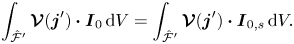 \begin{equation} \int_{\hat{\mathcal{F}}'}\boldsymbol{\mathcal{V}}(\boldsymbol{j}') \boldsymbol{\cdot}\boldsymbol{I}_{0} \,{\rm d}V = \int_{\hat{\mathcal{F}}'}\boldsymbol{\mathcal{V}}(\boldsymbol{j}') \boldsymbol{\cdot}\boldsymbol{I}_{0,s} \,{\rm d}V. \end{equation}
Analogous simplifications can be made for a number of other volume integrals involving a dot product between a  $\boldsymbol {\mathcal {V}}$ term and $\boldsymbol {I}_0$.
Upon applying these symmetry properties to (4.6) and (4.7) we arrive at
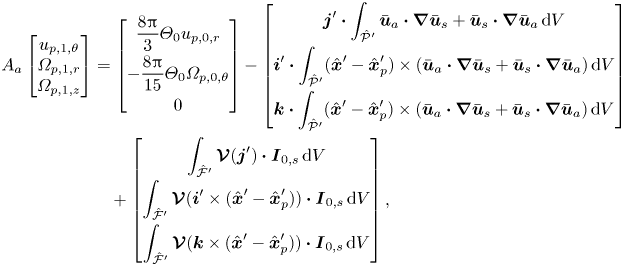 \begin{align} A_a\begin{bmatrix}
u_{p,1,\theta} \\ \varOmega_{p,1,r} \\ \varOmega_{p,1,z}
\end{bmatrix} &= \begin{bmatrix}
\dfrac{8{\rm \pi}}{3}\varTheta_0 u_{p,0,r} \\
-\dfrac{8{\rm \pi}}{15}\varTheta_{0}\varOmega_{p,0,\theta} \\ 0
\end{bmatrix}-\begin{bmatrix}
\displaystyle\boldsymbol{j}'\boldsymbol{\cdot}\int_{\hat{\mathcal{P}}'}\bar{\boldsymbol{u}}_a\boldsymbol{\cdot}\boldsymbol{\nabla}\bar{\boldsymbol{u}}_s+\bar{\boldsymbol{u}}_s\boldsymbol{\cdot}\boldsymbol{\nabla}\bar{\boldsymbol{u}}_a\,{\rm
d}V \\
\displaystyle\boldsymbol{i}'\boldsymbol{\cdot}\int_{\hat{\mathcal{P}}'}(\hat{\boldsymbol{x}}'-\hat{\boldsymbol{x}}_{p}^{\prime})\times(\bar{\boldsymbol{u}}_a\boldsymbol{\cdot}\boldsymbol{\nabla}\bar{\boldsymbol{u}}_s+\bar{\boldsymbol{u}}_s\boldsymbol{\cdot}\boldsymbol{\nabla}\bar{\boldsymbol{u}}_a)\,{\rm
d}V \\
\displaystyle\boldsymbol{k}\boldsymbol{\cdot}\int_{\hat{\mathcal{P}}'}(\hat{\boldsymbol{x}}'-\hat{\boldsymbol{x}}_{p}^{\prime})\times(\bar{\boldsymbol{u}}_a\boldsymbol{\cdot}\boldsymbol{\nabla}\bar{\boldsymbol{u}}_s+\bar{\boldsymbol{u}}_s\boldsymbol{\cdot}\boldsymbol{\nabla}\bar{\boldsymbol{u}}_a)\,{\rm
d}V \end{bmatrix} \nonumber\\ &\quad +\begin{bmatrix}
\displaystyle\int_{\hat{\mathcal{F}}'}\boldsymbol{\mathcal{V}}(\boldsymbol{j}')\boldsymbol{\cdot}\boldsymbol{I}_{0,s}
\,{\rm d}V \\
\displaystyle\int_{\hat{\mathcal{F}}'}\boldsymbol{\mathcal{V}}(\boldsymbol{i}'\times(\hat{\boldsymbol{x}}'-\hat{\boldsymbol{x}}_{p}^{\prime}))\boldsymbol{\cdot}\boldsymbol{I}_{0,s}
\,{\rm d}V \\
\displaystyle\int_{\hat{\mathcal{F}}'}\boldsymbol{\mathcal{V}}(\boldsymbol{k}\times(\hat{\boldsymbol{x}}'-\hat{\boldsymbol{x}}_{p}^{\prime}))\boldsymbol{\cdot}\boldsymbol{I}_{0,s}\,{\rm
d}V \end{bmatrix}, \end{align}
\begin{align} A_a\begin{bmatrix}
u_{p,1,\theta} \\ \varOmega_{p,1,r} \\ \varOmega_{p,1,z}
\end{bmatrix} &= \begin{bmatrix}
\dfrac{8{\rm \pi}}{3}\varTheta_0 u_{p,0,r} \\
-\dfrac{8{\rm \pi}}{15}\varTheta_{0}\varOmega_{p,0,\theta} \\ 0
\end{bmatrix}-\begin{bmatrix}
\displaystyle\boldsymbol{j}'\boldsymbol{\cdot}\int_{\hat{\mathcal{P}}'}\bar{\boldsymbol{u}}_a\boldsymbol{\cdot}\boldsymbol{\nabla}\bar{\boldsymbol{u}}_s+\bar{\boldsymbol{u}}_s\boldsymbol{\cdot}\boldsymbol{\nabla}\bar{\boldsymbol{u}}_a\,{\rm
d}V \\
\displaystyle\boldsymbol{i}'\boldsymbol{\cdot}\int_{\hat{\mathcal{P}}'}(\hat{\boldsymbol{x}}'-\hat{\boldsymbol{x}}_{p}^{\prime})\times(\bar{\boldsymbol{u}}_a\boldsymbol{\cdot}\boldsymbol{\nabla}\bar{\boldsymbol{u}}_s+\bar{\boldsymbol{u}}_s\boldsymbol{\cdot}\boldsymbol{\nabla}\bar{\boldsymbol{u}}_a)\,{\rm
d}V \\
\displaystyle\boldsymbol{k}\boldsymbol{\cdot}\int_{\hat{\mathcal{P}}'}(\hat{\boldsymbol{x}}'-\hat{\boldsymbol{x}}_{p}^{\prime})\times(\bar{\boldsymbol{u}}_a\boldsymbol{\cdot}\boldsymbol{\nabla}\bar{\boldsymbol{u}}_s+\bar{\boldsymbol{u}}_s\boldsymbol{\cdot}\boldsymbol{\nabla}\bar{\boldsymbol{u}}_a)\,{\rm
d}V \end{bmatrix} \nonumber\\ &\quad +\begin{bmatrix}
\displaystyle\int_{\hat{\mathcal{F}}'}\boldsymbol{\mathcal{V}}(\boldsymbol{j}')\boldsymbol{\cdot}\boldsymbol{I}_{0,s}
\,{\rm d}V \\
\displaystyle\int_{\hat{\mathcal{F}}'}\boldsymbol{\mathcal{V}}(\boldsymbol{i}'\times(\hat{\boldsymbol{x}}'-\hat{\boldsymbol{x}}_{p}^{\prime}))\boldsymbol{\cdot}\boldsymbol{I}_{0,s}
\,{\rm d}V \\
\displaystyle\int_{\hat{\mathcal{F}}'}\boldsymbol{\mathcal{V}}(\boldsymbol{k}\times(\hat{\boldsymbol{x}}'-\hat{\boldsymbol{x}}_{p}^{\prime}))\boldsymbol{\cdot}\boldsymbol{I}_{0,s}\,{\rm
d}V \end{bmatrix}, \end{align}
and similarly
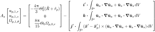 \begin{align} A_s\begin{bmatrix}
u_{p,1,r} \\ u_{p,1,z} \\ \varOmega_{p,1,\theta}
\end{bmatrix} &= \begin{bmatrix}
-\dfrac{4{\rm \pi}}{3}\varTheta_{0}^{2}(\hat{R}+\hat{r}_{p}) \\
0 \\ \dfrac{8{\rm \pi}}{15}\varTheta_{0}\varOmega_{p,0,r}
\end{bmatrix} -\begin{bmatrix}
\displaystyle\boldsymbol{i}'\boldsymbol{\cdot}\int_{\hat{\mathcal{P}}'}\bar{\boldsymbol{u}}_a\boldsymbol{\cdot}\boldsymbol{\nabla}\bar{\boldsymbol{u}}_a+\bar{\boldsymbol{u}}_s\boldsymbol{\cdot}\boldsymbol{\nabla}\bar{\boldsymbol{u}}_s\,{\rm
d}V \\
\displaystyle\boldsymbol{k}\boldsymbol{\cdot}\int_{\hat{\mathcal{P}}'}\bar{\boldsymbol{u}}_a\boldsymbol{\cdot}\boldsymbol{\nabla}\bar{\boldsymbol{u}}_a+\bar{\boldsymbol{u}}_s\boldsymbol{\cdot}\boldsymbol{\nabla}\bar{\boldsymbol{u}}_s\,{\rm
d}V \\
\displaystyle\boldsymbol{j}'\boldsymbol{\cdot}\int_{\hat{\mathcal{P}}'}(\hat{\boldsymbol{x}}'-\hat{\boldsymbol{x}}_{p}^{\prime})\times(\bar{\boldsymbol{u}}_a\boldsymbol{\cdot}\boldsymbol{\nabla}\bar{\boldsymbol{u}}_a+\bar{\boldsymbol{u}}_s\boldsymbol{\cdot}\boldsymbol{\nabla}\bar{\boldsymbol{u}}_s)\,{\rm
d}V \end{bmatrix} \nonumber\\ &\quad +\begin{bmatrix}
\displaystyle\int_{\hat{\mathcal{F}}'}\boldsymbol{\mathcal{V}}(\boldsymbol{i}')\boldsymbol{\cdot}\boldsymbol{I}_{0,a}
\,{\rm d}V \\
\displaystyle\int_{\hat{\mathcal{F}}'}\boldsymbol{\mathcal{V}}(\boldsymbol{k})\boldsymbol{\cdot}\boldsymbol{I}_{0,a}
\,{\rm d}V \\
\displaystyle\int_{\hat{\mathcal{F}}'}\boldsymbol{\mathcal{V}}(\boldsymbol{j}'\times(\hat{\boldsymbol{x}}'-\hat{\boldsymbol{x}}_{p}^{\prime}))\boldsymbol{\cdot}\boldsymbol{I}_{0,a}\,{\rm
d}V \end{bmatrix}. \end{align}
\begin{align} A_s\begin{bmatrix}
u_{p,1,r} \\ u_{p,1,z} \\ \varOmega_{p,1,\theta}
\end{bmatrix} &= \begin{bmatrix}
-\dfrac{4{\rm \pi}}{3}\varTheta_{0}^{2}(\hat{R}+\hat{r}_{p}) \\
0 \\ \dfrac{8{\rm \pi}}{15}\varTheta_{0}\varOmega_{p,0,r}
\end{bmatrix} -\begin{bmatrix}
\displaystyle\boldsymbol{i}'\boldsymbol{\cdot}\int_{\hat{\mathcal{P}}'}\bar{\boldsymbol{u}}_a\boldsymbol{\cdot}\boldsymbol{\nabla}\bar{\boldsymbol{u}}_a+\bar{\boldsymbol{u}}_s\boldsymbol{\cdot}\boldsymbol{\nabla}\bar{\boldsymbol{u}}_s\,{\rm
d}V \\
\displaystyle\boldsymbol{k}\boldsymbol{\cdot}\int_{\hat{\mathcal{P}}'}\bar{\boldsymbol{u}}_a\boldsymbol{\cdot}\boldsymbol{\nabla}\bar{\boldsymbol{u}}_a+\bar{\boldsymbol{u}}_s\boldsymbol{\cdot}\boldsymbol{\nabla}\bar{\boldsymbol{u}}_s\,{\rm
d}V \\
\displaystyle\boldsymbol{j}'\boldsymbol{\cdot}\int_{\hat{\mathcal{P}}'}(\hat{\boldsymbol{x}}'-\hat{\boldsymbol{x}}_{p}^{\prime})\times(\bar{\boldsymbol{u}}_a\boldsymbol{\cdot}\boldsymbol{\nabla}\bar{\boldsymbol{u}}_a+\bar{\boldsymbol{u}}_s\boldsymbol{\cdot}\boldsymbol{\nabla}\bar{\boldsymbol{u}}_s)\,{\rm
d}V \end{bmatrix} \nonumber\\ &\quad +\begin{bmatrix}
\displaystyle\int_{\hat{\mathcal{F}}'}\boldsymbol{\mathcal{V}}(\boldsymbol{i}')\boldsymbol{\cdot}\boldsymbol{I}_{0,a}
\,{\rm d}V \\
\displaystyle\int_{\hat{\mathcal{F}}'}\boldsymbol{\mathcal{V}}(\boldsymbol{k})\boldsymbol{\cdot}\boldsymbol{I}_{0,a}
\,{\rm d}V \\
\displaystyle\int_{\hat{\mathcal{F}}'}\boldsymbol{\mathcal{V}}(\boldsymbol{j}'\times(\hat{\boldsymbol{x}}'-\hat{\boldsymbol{x}}_{p}^{\prime}))\boldsymbol{\cdot}\boldsymbol{I}_{0,a}\,{\rm
d}V \end{bmatrix}. \end{align}
This decomposition illustrates a clear separation in how different parts of the leading-order disturbance flow solution contribute to the hydrodynamic force generated by the first-order disturbance flow correction. In (C4) and (C5), the  $\bar {\boldsymbol {u}}_a$ should be interpreted as $\bar {\boldsymbol {u}}_{a,0}+K\bar {\boldsymbol {u}}_{a,1}+K^2\bar {\boldsymbol {u}}_{a,2}$ and similarly for $\bar {\boldsymbol {u}}_s$. Both $\boldsymbol {v}_{0,a},\boldsymbol {v}_{0,s}$ from (C1) can be substituted into $\boldsymbol {I}_{0,a},\boldsymbol {I}_{0,s}$ in (C2), and subsequently the volume integrals over $\hat {\mathcal {F}}'$ in (C4) and (C5) can be expressed as a polynomial function of $\boldsymbol {u}_{p,0},\boldsymbol {\varOmega }_{p,0},\varTheta _0,\kappa,\textit {Re}_p,K$ with variable coefficients depending on $r_p,z_p,\epsilon,\alpha$. By sampling the coefficient fields over a suitable range of $r_p,z_p,\epsilon,\alpha$ and interpolating appropriately, we can efficiently estimate the values of $\boldsymbol {u}_{p,1},\boldsymbol {\varOmega }_{p,1}$ given any value of $\boldsymbol {u}_{p,0},\boldsymbol {\varOmega }_{p,0},\varTheta _0,\kappa,\textit {Re}_p,K$ (assuming $\textit {Re}_p$ and $K$ are small enough that the regular perturbation expansion is valid).


 Open access