


NOMENCLATURE
-
 $A_{\rm c}$
-
sectorial area
- ()′
differentiation with respect to spanwise coordinate
-
$\theta_x$
-
rotation about x axis
-
$\theta_y$
-
rotation about y axis
-
$\phi$
-
twist about z axis
-
$F_{\omega}$
-
primary warping function
-
$\psi$
-
torsional function
-
$\epsilon_{xz},\epsilon_{yz}$
-
transverse shear strains
-
$F_{\omega}$
-
primary warping function
- s
-
contour coordinate
- n
-
coordinate in wall thickness direction
-
$u_0 , v_0,w_0$
-
rigid-body translation along x,y,z axis
-
$\bar{Q}_{ij}$
-
modified transformed stiffness
-
${Q}_{ij}$
-
transformed stiffness
-
$ E_i$
-
Young’s modulus
- G
-
shear modulus
-
$\nu$
-
Poisson’s ratio
- L
-
length of the beam
- D
-
material stiffness matrix
- N
-
shape function
- K
-
stiffness matrix of the beam element
- CUS
-
circumferentially uniform stiffness
- CAS
-
circumferentially asymmetric stiffness


1.0 INTRODUCTION
Recently, composite materials have gained popularity for use in various industrial applications due to advances in composite manufacturing as well as their attractive weight-to-strength ratio and enhanced damage and fatigue behaviour. Composite structures will play a significant role in achieving the ambitious carbon emission targets set by the International Air Transport Authority (IATA)(Reference Bisignani1). More than 50% of the structural weight of modern-day aircraft such as the Boeing 787 and Airbus A350 XWB consists of composite structures. Many primary composite structures such as helicopter blades and aircraft wings can be analysed by modelling them as thin-walled composite beams. Further application of advanced composites is expected to reduce structural weight and improve aerodynamics, both aspects leading to reduced fuel consumption. To optimally design such composite structures, one has to utilise the full extent of the tailorability offered by composites. In particular, the elastic coupling between the different displacement fields inherent to thin-walled beams and the resulting non-classical effects must be analysed and incorporated into the overall aircraft design process.
To accurately predict the beam’s behaviour, a correct representation of the 3D motion into the 1D mathematical beam theory is of critical importance. Analytical models and variational asymptomatic beam sectional analysis are two approaches that can be used to capture the non-classical effects of composite beams. During the past few decades, there has been a steady increase in investigations on laminated composite beams with closed and open cross-section(Reference Bauld and Lih-Shyng2–Reference Vo and Lee8). Some of the earliest studies modelling the composite structure as a 1D beam were performed by Sobey et al.(Reference Mansfield and Sobey9,Reference Mansfield10) , who developed the theory of thin-walled cylindrical tubes and aeroelasticity tailored composite helicopter blades, albeit with a simplified cross-sectional analysis. More refined cross-sectional analysis based on the two-dimensional finite element method, commonly known as Variational Asymptotic Beam Section (VABS) analysis, was developed by Hodges et al.(Reference Cesnik and Hodges3). Several researchers have developed analytical cross-sectional models for evaluating the constitutive equation for the beam(Reference Smith and Chopra5,Reference Chandra and Chopra11,Reference Salim and Davalos12) . Jung et al. formulated a first-order shear-deformable analytical cross-sectional modelling technique(Reference Jung, Nagaraj and Chopra13). An exhaustive survey of different thin-walled beam theories was carried out by Jung et al.(Reference Jung, Nagaraj and Chopra14,Reference Jung, Nagaraj and Chopra15) .
Composite materials usually have very low traverse shear modulus as compared with their extensional shear modulus, thus transverse shear effects are significant for laminated composite structures. Therefore, shear-deformable theories are more suitable for accurately predicting their behaviour. In shear-deformable theories such as First-Order Shear-Deformable Theories (FSDTs), the transverse displacement and slope must be interpolated using
 $C^0$
. However, it is well known that these
$C^0$
. However, it is well known that these
 $C^0$
elements are accompanied by shear constraints. Therefore, under certain limiting conditions, e.g. thin beams, the shear constraints do not yield zero shear strains, resulting in the problem of shear locking. These finite element formulations are thus termed inconsistent, and selective or reduced integration can be applied to address the locking problem(Reference Reddy16,Reference Hughes, Cohen and Haroun17) . Alternatively, a consistent finite element method can be formulated by constructing shape functions from the general solutions to the homogeneous Euler–Lagrange equations(Reference Yunhua18). Such an approach has been implemented to obtain the shape function for an isotropic 3D Timoshenko beam element(Reference Luo19). Eisenberger(Reference Eisenberger20) formulated a strategy for obtaining the exact stiffness matrix for the higher-order isotropic beam. The unique feature of these elements is the dependence of the constants of the interpolating polynomials on the material and the cross-sectional properties. Moreover, the user does not have to judge whether the shear deformation in the element is significant. However, all these beam models are isotropic. With the advances of computing hardware, the complex and highly coupled homogeneous Euler–Lagrangian equations governing the composite thin-walled beam can be solved by using modern mathematical software such as Maple and Mathematica in a similar manner to their isotropic counterparts(Reference Luo19). Such an analytical approach to solving the governing equations would not have been possible a few years ago. The aim of the current work is to develop the governing equations and obtain corresponding consistent shape functions analytically.
$C^0$
elements are accompanied by shear constraints. Therefore, under certain limiting conditions, e.g. thin beams, the shear constraints do not yield zero shear strains, resulting in the problem of shear locking. These finite element formulations are thus termed inconsistent, and selective or reduced integration can be applied to address the locking problem(Reference Reddy16,Reference Hughes, Cohen and Haroun17) . Alternatively, a consistent finite element method can be formulated by constructing shape functions from the general solutions to the homogeneous Euler–Lagrange equations(Reference Yunhua18). Such an approach has been implemented to obtain the shape function for an isotropic 3D Timoshenko beam element(Reference Luo19). Eisenberger(Reference Eisenberger20) formulated a strategy for obtaining the exact stiffness matrix for the higher-order isotropic beam. The unique feature of these elements is the dependence of the constants of the interpolating polynomials on the material and the cross-sectional properties. Moreover, the user does not have to judge whether the shear deformation in the element is significant. However, all these beam models are isotropic. With the advances of computing hardware, the complex and highly coupled homogeneous Euler–Lagrangian equations governing the composite thin-walled beam can be solved by using modern mathematical software such as Maple and Mathematica in a similar manner to their isotropic counterparts(Reference Luo19). Such an analytical approach to solving the governing equations would not have been possible a few years ago. The aim of the current work is to develop the governing equations and obtain corresponding consistent shape functions analytically.
Automatic Differentiation (AD) is popular for the automation of derivative calculations in numerical optimisation, being preferred over other traditional methods for the differentiation of complex functions and algorithms. However, the implementation of AD requires significant effort and development time to ensure efficiency. Naively implemented AD can yield inefficient code, and significant computational cost(Reference Margossian21). One of the goals of the present work is to address the disadvantages of AD in optimisation involving composite thin-walled structures, e.g. aero-structural optimisation of composite surfaces. The methodology implemented herein ensures the availability of analytical shape functions for laminated composite thin-walled beams. Moreover, the derivatives of the shape functions can also be obtained easily by symbolic differentiation. In this way, the need for AD implementation and the associated pitfalls are eliminated, and optimisation can be performed robustly.
The modelling approach applied herein is based on field-consistent formulations; i.e. the interdependence of the beam displacements on each other is taken into account. The local displacements are obtained from the generalised beam displacements. The reduced constitutive equation for an arbitrary cross-section beam is derived based on the assumption of plane stress. The strain energies are evaluated in terms of beam displacements. The governing equations are derived by integration by parts of the expression for the strain energies. The homogeneous equations are then solved using Maple mathematical software to obtain the interpolating shape functions for the beam displacements.
The remainder of this manuscript is organised as follows: First, the kinematic description of the 1D beam representing the 3D motion is explained. After that, the constitutive relationship for a composite beam with arbitrary cross-section and laminate layup is derived. In the next section, expressions for the strain energy and governing equations, then the formulation of the stiffness matrix of the beam element is derived. Finally, the super-convergent property of the beam element is illustrated. The numerical results obtained using the developed beam element are then compared with experimental and numerical results from literature.
2.0 KINEMATICS OF THIN-WALLED BEAMS
In the present work, the case of thin-walled beams with arbitrary closed cross-section is considered. The kinematics of the thin-walled beams are derived by adopting a number of assumptions:
-
(i) The projection of the cross-section onto a plane normal to the z-axis does not distort during deformations. This implies that the original cross-sections do not deform in their planes.
-
(ii) Transverse shear effects are considered, and the shear strains
$\epsilon_{xz}$
and
$\epsilon_{yz}$
are uniform through the wall thickness(Reference Rehfield22). -
(iii) The warping displacements along the mid-line contour (referred to as primary warping) and off the mid-line contour (referred to as secondary warping) are incorporated(Reference Rehfield, Atilgan and Hodges4,Reference Librescu and Song6,Reference Rehfield22,Reference Bauchau, Coffenberry and Rehfield23) .


The effect of the primary warping is usually quantified by a function called the primary warping function and denoted by
 $F_{\omega}$
, defined as(Reference Librescu and Song6,Reference Megson24,Reference Song and Librescu25)
$F_{\omega}$
, defined as(Reference Librescu and Song6,Reference Megson24,Reference Song and Librescu25)
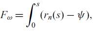 \begin{align} \begin{split} F_{\omega} = \int_{0}^{s} ( r_n (s) - \psi), \end{split} \end{align}
where the torsional function
 $\psi$
is given by Ref.(Reference Song and Librescu25)
$\psi$
is given by Ref.(Reference Song and Librescu25)
 \begin{align} \begin{split} \psi = \dfrac{\oint \, r_n(s) \mathrm{d}s}{\oint \mathrm{d}s} = \dfrac{2A_{\rm c}}{\beta}, \\ \end{split}\end{align}
where
 $ A_{\rm c} $
denotes the cross-sectional area bounded by the mid-line contour, and s is the circumferential coordinate as shown in Fig. 1. The circumferential coordinate s corresponds to the mid-line of the beam cross-section walls. The geometrical quantity
$ A_{\rm c} $
denotes the cross-sectional area bounded by the mid-line contour, and s is the circumferential coordinate as shown in Fig. 1. The circumferential coordinate s corresponds to the mid-line of the beam cross-section walls. The geometrical quantity
 $ r_n $
is given by
$ r_n $
is given by
Figure 1. Coordinate system.
 \begin{equation} r_n = x(s) \, \dfrac{\mathrm{d}y}{\mathrm{d}s} - y(s) \, \dfrac{\mathrm{d}x}{\mathrm{d}s} \end{equation}
Based on assumptions (i), (ii) and (iii) and representing the 3D motion of the beam by an equivalent 1D beam, the displacement of any point on the mid-line contour can be expressed as(Reference Song and Librescu25)
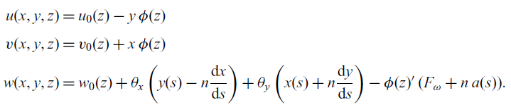 \begin{align} \begin{split} u(x,y,z) &= u_0(z) - y \, \phi(z)\\[3pt] v(x,y,z) &= v_0(z) + x \, \phi(z) \\[3pt] w(x,y,z) &= w_0 (z)+ \theta_x \, \bigg( y(s) - n \dfrac{\mathrm{d}x}{\mathrm{d}s} \bigg) + \theta_y \, \bigg( x(s) + n \dfrac{\mathrm{d}y}{\mathrm{d}s} \bigg) - \phi(z)' \, ( F_{\omega} + n \, a(s) ). \end{split}\end{align}
The term
 $n \, a(s) \, \phi(z)' $
accounts for the secondary warping effects, where the prime represents the derivative with respect to z.
$n \, a(s) \, \phi(z)' $
accounts for the secondary warping effects, where the prime represents the derivative with respect to z.
 $u_0, v_0 $
and
$u_0, v_0 $
and
 $ w_0 $
denote rigid-body translations. The subscript ‘0’ is dropped hereinafter for the sake of brevity. The rotations
$ w_0 $
denote rigid-body translations. The subscript ‘0’ is dropped hereinafter for the sake of brevity. The rotations
 $\theta_x$
and
$\theta_x$
and
 $\theta_y$
and the geometrical quantity a are expressed as
$\theta_y$
and the geometrical quantity a are expressed as
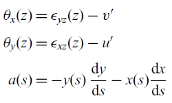 \begin{align} \begin{split} \theta_x(z) &= \epsilon_{yz}(z) - v' \\[3pt] \theta_y(z) &= \epsilon_{xz}(z) - u' \\[3pt] a(s) &= -y(s) \, \dfrac{\mathrm{d}y}{\mathrm{d}s} - x(s) \dfrac{\mathrm{d}x}{\mathrm{d}s} \end{split}\end{align}
From Equations (4) and (5), it is clear that the strain components
 $\epsilon_{xx} , \epsilon_{yy},\epsilon_{xy}$
are zero. This implies that the strain components in the local coordinate system,
$\epsilon_{xx} , \epsilon_{yy},\epsilon_{xy}$
are zero. This implies that the strain components in the local coordinate system,
 $s-n$
(
$s-n$
(
 $\epsilon_{nn}$
,
$\epsilon_{nn}$
,
 $\epsilon_{ss},\epsilon_{sn}$
), are also zero. Thus, the condition of cross-section non-deformability in assumption (i) is satisfied. Consequently, the three non-trivial strains for the 3D beam are
$\epsilon_{ss},\epsilon_{sn}$
), are also zero. Thus, the condition of cross-section non-deformability in assumption (i) is satisfied. Consequently, the three non-trivial strains for the 3D beam are
 $\epsilon_{zz} , \epsilon_{zs}$
and
$\epsilon_{zz} , \epsilon_{zs}$
and
 $\epsilon_{zn} $
.
$\epsilon_{zn} $
.
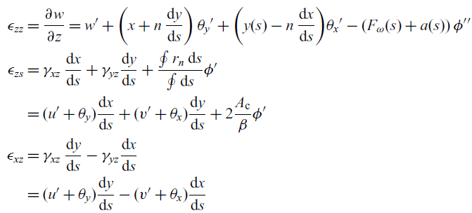
 $\epsilon_{zz}$
denotes the axial strain component, while
$\epsilon_{zz}$
denotes the axial strain component, while
 $\epsilon_{zs}$
and
$\epsilon_{zs}$
and
 $\epsilon_{zn}$
denote the membrane and transverse shear strain, respectively. The strains are assumed to be small, so a linear strain–displacement relationship can be adopted. The strain measure in the beam can be calculated using the definition of the linear strain–displacement relations and Equation (4) and (5)(Reference Librescu and Song6):
$\epsilon_{zn}$
denote the membrane and transverse shear strain, respectively. The strains are assumed to be small, so a linear strain–displacement relationship can be adopted. The strain measure in the beam can be calculated using the definition of the linear strain–displacement relations and Equation (4) and (5)(Reference Librescu and Song6):
 \begin{align} \begin{split} \epsilon_{zz} &= \dfrac{\partial w }{\partial z} = w' + \bigg( x + n\, \dfrac{\mathrm{d}y}{\mathrm{d}s}\bigg) \, \theta_y' + \bigg( y(s) - n \, \dfrac{\mathrm{d}x}{\mathrm{d}s} \bigg)\theta_x' - (F_\omega(s) + a(s))\, \phi'' \\ \epsilon_{zs} &= \gamma_{xz} \, \dfrac{\mathrm{d}x}{\mathrm{d}s} + \gamma_{yz} \dfrac{\mathrm{d}y}{\mathrm{d}s} + \dfrac{\oint r_n \, \mathrm{d}s}{\oint \mathrm{d}s} \phi' \\ &= (u' + \theta_y) \dfrac{\mathrm{d}x}{\mathrm{d}s} + (v' + \theta_x) \dfrac{\mathrm{d}y}{\mathrm{d}s} + 2 \dfrac{A_{\rm c}}{\beta} \phi' \\ \epsilon_{xz} &= \gamma_{xz} \, \dfrac{\mathrm{d}y}{\mathrm{d}s} - \gamma_{yz} \dfrac{\mathrm{d}x}{\mathrm{d}s} \\ &=(u' + \theta_y) \dfrac{\mathrm{d}y}{\mathrm{d}s} - (v' + \theta_x) \dfrac{\mathrm{d}x}{\mathrm{d}s} \end{split}\end{align}
3.0 CONSTITUTIVE RELATIONSHIPS
The Two-Dimensional (2D) behaviour of composite plies must be treated adequately within the one-dimensional beam model. In particular, the in-plane elastic behaviour of laminates must be considered in the beam model. Three different methods accounting for in-plane elastic behaviour were investigated by Smith et al.(Reference Chandra and Chopra11). In one-dimensional beam theory, it is reasonable to assume that the transverse in-plane stress
 $\sigma_{ss}$
is negligibly small compared with the other stress components. Consequently, the reduced constitutive equation for a particular ply is obtained as
$\sigma_{ss}$
is negligibly small compared with the other stress components. Consequently, the reduced constitutive equation for a particular ply is obtained as
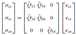 \begin{equation} \begin{bmatrix} \sigma_{zz} \\[10pt] \sigma_{zs} \\[10pt] \sigma_{zn} \end{bmatrix} = \begin{bmatrix} \bar{Q}_{11} & \bar{Q}_{16} & 0 \\[10pt] \bar{Q}_{16} & \bar{Q}_{66} & 0 \\[10pt] 0 & 0 & \bar{Q}_{55} \end{bmatrix} \begin{bmatrix} \epsilon_{zz} \\[10pt] \epsilon_{zs} \\[10pt] \epsilon_{zn} \end{bmatrix}\end{equation}
In Equation (7), the terms
 $\bar{Q}_{ij}$
, commonly referred to as the modified transformed stiffness coefficients, are derived from the conventional transformed coefficients
$\bar{Q}_{ij}$
, commonly referred to as the modified transformed stiffness coefficients, are derived from the conventional transformed coefficients
 $Q_{ij}$
(Reference Smith and Chopra5) as follows:
$Q_{ij}$
(Reference Smith and Chopra5) as follows:
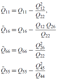 \begin{align} \begin{split} \bar{Q}_{11} &= Q_{11} - \dfrac{Q_{12}^2}{Q_{22}} , \\[3pt] \bar{Q}_{16} &= Q_{16} - \dfrac{Q_{12} \, Q_{26}}{Q_{22}} \\[3pt] \bar{Q}_{66} &= Q_{66} - \dfrac{Q_{26}^2}{Q_{22}} \\[3pt] \bar{Q}_{55} &= Q_{55} - \dfrac{Q_{45}^2}{Q_{44}} \\[3pt] \end{split}\end{align}
For a given ply laminate angle
 $\alpha$
and material properties, the
$\alpha$
and material properties, the
 $ Q_{ij} $
are obtained as
$ Q_{ij} $
are obtained as
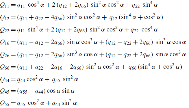 \begin{align} \begin{split} {Q}_{11} &= q_{11} \, \cos^4\alpha + 2\,(q_{12} + 2q_{66})\, \sin^2\alpha \cos^2\alpha + q_{22}\, \sin^4\alpha \\[3pt] {Q}_{12} &= (q_{11} + q_{22} - 4q_{66} )\, \sin^2\alpha \cos^2\alpha + \,q_{12} \,( \sin^4\alpha + \cos^2\alpha) \\[3pt] {Q}_{22} &= q_{11} \, \sin^4\alpha + 2\,(q_{12} + 2q_{66})\, \sin^2\alpha \cos^2\alpha + q_{22}\, \cos^4\alpha \\[3pt] {Q}_{16} &= (q_{11} - q_{12} - 2q_{66} )\, \sin\alpha \cos^3\alpha +(q_{12} - q_{22} +2q_{66} )\, \sin^3\alpha \cos\alpha \\[3pt] {Q}_{26} &= (q_{11} - q_{12} - 2q_{66} )\, \sin^3\alpha \cos\alpha +(q_{12} - q_{22} +2q_{66} )\, \sin\alpha \cos^3\alpha \\[3pt] {Q}_{66} &= (q_{11} + q_{22} - 2q_{16} -2q_{66})\, \sin^2\alpha \cos^2\alpha + \,q_{66} \,( \sin^4\alpha + \cos^2\alpha) \\[3pt] {Q}_{44} &= q_{44}\cos^2\alpha + \,q_{55} \, \sin^2\alpha \\[3pt] {Q}_{45} &= (q_{55} - q_{44})\cos\alpha \sin\alpha \\[3pt] {Q}_{55} &= q_{55}\, \cos^2\alpha + q_{44}\sin^2\alpha \\[3pt] \end{split}\end{align}
 $q_{ij}$
are related to engineering constants as follows:
$q_{ij}$
are related to engineering constants as follows:
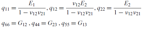 \begin{align} \begin{split} {q}_{11} &= \dfrac{E_{1}}{1-\nu_{12}\nu_{21}} ,{q}_{12} = \dfrac{\nu_{12}E_{2}}{1-\nu_{12}\nu_{21}} , {q}_{22} = \dfrac{E_{2}}{1-\nu_{12}\nu_{21}} \\[3pt] {q}_{66} &= G_{12} \, , {q}_{44} = G_{23} \,, {q}_{55} = G_{13} \\[3pt] \end{split}\end{align}
4.0 GOVERNING EQUATION OF MOTION AND FINITE ELEMENT FORMULATION
In the preceding sections, the kinematics and local constitutive relationships of a thin-walled laminated beam were presented. To obtain the governing equation of motion, the variation of the strain energy expression V is derived as
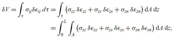 \begin{multline} \begin{split} \delta V = \int_{\tau} \sigma_{ij} \delta \epsilon_{ij} \, d\tau &= \int_{\tau} \big( \sigma_{zz} \, \delta \epsilon_{zz} + \sigma_{zs} \, \delta\epsilon_{zs} + \sigma_{zn} \, \delta \epsilon_{zn} \big) \, \mathrm{d}A \, \mathrm{d}z \\ &= \int_{0}^{L} \int_{A} \big( \sigma_{zz} \, \delta \epsilon_{zz} + \sigma_{zs} \, \delta\epsilon_{zs} + \sigma_{zn} \, \delta \epsilon_{zn} \big) \, \mathrm{d}A \, \mathrm{d}z, \end{split}\end{multline}
where
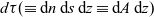 $d\tau (\equiv \mathrm{d}n\,\mathrm{d}s\,\mathrm{d}z \equiv \mathrm{d}A \,\mathrm{d}z)$
denotes the differential volume element and
$d\tau (\equiv \mathrm{d}n\,\mathrm{d}s\,\mathrm{d}z \equiv \mathrm{d}A \,\mathrm{d}z)$
denotes the differential volume element and
 $\delta$
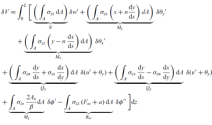
is the variation sign. Also, the Einstein summation convention applies for the indices i,j. Using the strain expressions from Equation (6) and local constitutive relationships from Equation (7), the variation of the virtual energy takes the form
$\delta$
is the variation sign. Also, the Einstein summation convention applies for the indices i,j. Using the strain expressions from Equation (6) and local constitutive relationships from Equation (7), the variation of the virtual energy takes the form
 \begin{align} \delta V &= \int^L_0\bigg[\underbrace{\bigg(\int_{A}\sigma_{zz} \,\mathrm{d}A \bigg)}_N \delta{w'} + \underbrace{\bigg(\int_{A}\sigma_{zz} \, \bigg(x + n \dfrac{\mathrm{d}y}{\mathrm{d}s}\bigg) \,dA \bigg)}_{M_y} \, \delta{\theta}_y' \nonumber\\ &\quad + \underbrace{\bigg(\int_{A}\sigma_{zz} \, \bigg(y - n\, \dfrac{\mathrm{d}x}{\mathrm{d}s}\bigg) \,\mathrm{d}A \bigg) }_{M_x} \,\delta {\theta_x}' \nonumber \\ &\quad + \underbrace{\bigg(\int_{A} \sigma_{zn} \,\dfrac{\mathrm{d}y}{\mathrm{d}s} + \sigma_{zs}\, \dfrac{\mathrm{d}x}{\mathrm{d}y} \bigg)\, \mathrm{d}A }_{Q_x} \,\delta{(u' + \theta_y)} + \underbrace{\bigg(\int_{A} \sigma_{zs} \,\dfrac{\mathrm{d}y}{\mathrm{d}s} - \sigma_{zn}\, \dfrac{\mathrm{d}x}{\mathrm{d}y} \bigg) \, \mathrm{d}A}_{Q_y} \,\delta{(v' + \theta_y)} \nonumber\\ &\quad + \underbrace{ \int_{A} \sigma_{zs} \, \dfrac{2A_{\rm c}}{\beta} \mathrm{d}A }_{M_z} \, \delta{\phi'} - \underbrace{\int_{A} \sigma_{zz} \, (F_\omega +a )\,\mathrm{d}A }_{B_\omega} \, \delta\phi'' \, \bigg] \mathrm{d}z \end{align}
In Equation (12), the integration is first performed over the cross-section area A, then in subsequent steps, the integration is performed along the span of the beam L. Based on the formulation in Equation (12), stress resultants can be calculated.
 $N , Q_y$
and
$N , Q_y$
and
 $Q_z $
represent the axial and shear forces in the x and y direction, respectively.
$Q_z $
represent the axial and shear forces in the x and y direction, respectively.
 $M_x , M_y , Q_z$
and
$M_x , M_y , Q_z$
and
 $ B_\omega$
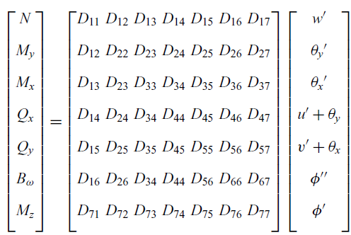
represent the moments about the x, y and z-axis and global bi-moment, respectively. Considering Equations (6) and (7) in conjunction with the stress resultant definitions in Equation (12), the material stiffness D can be obtained.
$ B_\omega$
represent the moments about the x, y and z-axis and global bi-moment, respectively. Considering Equations (6) and (7) in conjunction with the stress resultant definitions in Equation (12), the material stiffness D can be obtained.
 \begin{equation} \begin{bmatrix} N \\[8pt] M_y \\[8pt] M_x \\[8pt] Q_x \\[8pt] Q_y \\[8pt] B_\omega \\[8pt] M_z \\[8pt] \end{bmatrix} =\begin{bmatrix} {D}_{11} & {D}_{12} & {D}_{13} & {D}_{14} & {D}_{15} &{D}_{16} &{D}_{17} \\[8pt] {D}_{12} & {D}_{22} & {D}_{23} &{D}_{24} & {D}_{25} &{D}_{26}&{D}_{27} \\[8pt] {D}_{13} & {D}_{23} &{D}_{33} & {D}_{34} & {D}_{35} & {D}_{36}&{D}_{37} \\[8pt] {D}_{14} & {D}_{24} & {D}_{34} & {D}_{44} & D_{45} & {D}_{46}&{D}_{47} \\[8pt] {D}_{15} & {D}_{25} & {D}_{35} & D_{45} &{D}_{55} & {D}_{56} &{D}_{57} \\[8pt] {D}_{16} & {D}_{26} &{D}_{34} & {D}_{44} &{D}_{56} & {D}_{66}&{D}_{67} \\[8pt] {D}_{71} & {D}_{72} &{D}_{73} & {D}_{74} &{D}_{75} & {D}_{76}&{D}_{77} \\[8pt] \end{bmatrix} \begin{bmatrix} w' \\[8pt] \theta_y' \\[8pt] \theta_x' \\[8pt] u' + \theta_y \\[8pt] v' + \theta_x \\[8pt] \phi'' \\[8pt] \phi' \\[8pt] \end{bmatrix}\end{equation}
Expressions for the material stiffness matrix
 $\textbf{\textit{D}}$
are listed in the Appendix. It is clear from the derived stress resultants that, with arbitrary anisotropy, the composite laminated beam structure will exhibit complete elastic coupling between bending, warping, twist and transverse loading. These non-classical couplings should be fully understood to explore them effectively for optimum structural design.
$\textbf{\textit{D}}$
are listed in the Appendix. It is clear from the derived stress resultants that, with arbitrary anisotropy, the composite laminated beam structure will exhibit complete elastic coupling between bending, warping, twist and transverse loading. These non-classical couplings should be fully understood to explore them effectively for optimum structural design.
Note that the material stiffness matrix
 $\textbf{\textit{D}}$
(also commonly known as the cross-sectional stiffness matrix) is derived for a general arbitrary cross-section. This is evident from the kinematics discussion in Section 1.
$\textbf{\textit{D}}$
(also commonly known as the cross-sectional stiffness matrix) is derived for a general arbitrary cross-section. This is evident from the kinematics discussion in Section 1.
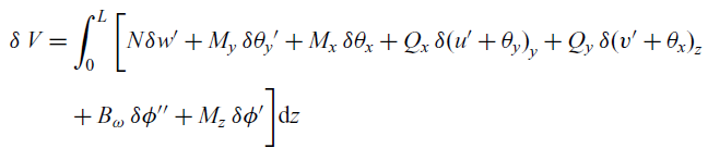
From Equations (12) and (13), the variation in the strain energy is
 \begin{align} \delta \, V &= \int_{0}^{L} \bigg[ N \delta{w'} + {M_y} \, \delta{\theta_y'} + {M_x} \,\delta {\theta_x} + {Q_x} \,\delta{(u' + \theta_y)}_y + Q_y \,\delta{(v' + \theta_x)}_z \nonumber\\[3pt] &\quad + {B_\omega} \, \delta{\phi''} + {M_z} \, \delta{\phi'}\bigg] \mathrm{d}z \end{align}
Combining Equations (14) and (13), we obtain
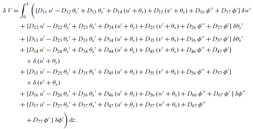 \begin{align} \delta \, V &= \int_{0}^{L} \bigg( \{D_{11} \, u' - D_{12} \, \theta_y' + D_{13}\, \theta_x' + D_{14}\, (u' + \theta_y) + D_{15}\, (v' + \theta_x) + D_{16} \, \phi'' + D_{17} \, \phi' \}\, \delta w' \nonumber \\[2pt] &\quad + \{D_{12} \, u' - D_{22} \, \theta_y' + D_{23}\, \theta_x' + D_{24}\, (u' + \theta_y) + D_{25}\, (v' + \theta_x) + D_{26} \, \phi'' + D_{27} \, \phi' \} \, \delta \theta_y' \nonumber \\[2pt] &\quad + \{D_{13} \, u' - D_{23} \, \theta_y' + D_{33}\, \theta_x' + D_{34}\, (u' + \theta_y) + D_{35}\, (v' + \theta_x) + D_{36} \, \phi'' + D_{37} \, \phi' \} \,\delta \theta_x' \nonumber\\[2pt] &\quad + \{ D_{14} \, u' - D_{24} \, \theta_y' + D_{34}\, \theta_x' + D_{44}\, (u' + \theta_y) + D_{45}\, (v' + \theta_x) + D_{46} \, \phi'' + D_{47} \, \phi' \}\nonumber\\[2pt] &\qquad \times \delta \, (u' +\theta_y) \, \nonumber\\[2pt] &\quad + \{D_{15} \, u' - D_{25} \, \theta_y' + D_{35}\, \theta_x' + D_{45}\, (u' + \theta_y) + D_{55}\, (v' + \theta_x) + D_{56} \, \phi'' + D_{57} \, \phi'\}\nonumber\\[2pt] &\qquad \times \delta \, (v' + \theta_x) \, \nonumber\\[2pt] &\quad + \{D_{16} \, u' - D_{26} \, \theta_y' + D_{36}\, \theta_x' + D_{46}\, (u' + \theta_y) + D_{56}\, ( w' + \theta_x ) + D_{66} \, \phi'' + D_{67} \, \phi' \, \} \, \delta \phi'' \nonumber\\[2pt] &\quad + \{D_{17} \, u' - D_{27} \, \theta_y' + D_{37}\, \theta_x' + D_{47}\, (u' + \theta_y) + D_{57}\, ( w' + \theta_x ) + D_{67} \, \phi'' \nonumber\\[2pt] &\qquad + D_{77} \, \phi' \, \} \, \delta \phi' \bigg)\,\mathrm{d}z. \end{align}
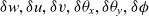
To obtain the governing equations, integration by parts is performed to relieve the virtual displacements (
 $\delta w , \delta u, \delta v, \delta \theta_x ,\delta \theta_y, \delta \phi$
) of any differentiation. Based on the principle of virtual work, the stored strain energy is equal to the virtual work performed by external forces. Using this principle and collecting terms corresponding to each virtual displacement, the homogeneous Euler–Lagrangian equations are obtained as
$\delta w , \delta u, \delta v, \delta \theta_x ,\delta \theta_y, \delta \phi$
) of any differentiation. Based on the principle of virtual work, the stored strain energy is equal to the virtual work performed by external forces. Using this principle and collecting terms corresponding to each virtual displacement, the homogeneous Euler–Lagrangian equations are obtained as
 \begin{align} \delta w :\, & D_{11} \, w'' + D_{12} \, \theta_y'' + D_{13}\, \theta_x'' + D_{14}\, ( \theta_y' + u'' ) + D_{15}\, ( \theta_x' + v'' ) + D_{16} \, \phi''' + D_{17} \, \phi'' = 0 \nonumber\\[5pt] \delta u :\, & D_{41} \, w'' + D_{42} \, \theta_y'' + D_{43}\, \theta_x'' + D_{44}\, ( u'' + \theta_y' ) + D_{45}\, ( v'' + \theta_x' ) + D_{46} \, \phi''' + D_{47} \, \phi'' = 0 \nonumber\\[5pt] \delta v :\, & D_{15} \, w'' + D_{25} \, \theta_y'' + D_{35}\, \theta_x'' + D_{45}\, ( u'' + \theta_y' ) + D_{55}\, ( v'' + \theta_x' ) + D_{56} \, \phi''' + D_{57} \, \phi'' = 0 \nonumber\\[5pt] \delta \theta_y :\, & D_{12} \, u'' + D_{22} \, \theta_y'' + D_{23}\, \theta_x'' + D_{24}\, ( u'' + \theta_y' ) + D_{25}\, ( v'' + \theta_x' ) + D_{26} \, \phi''' + D_{27} \, \phi'' \nonumber\\[5pt] & -D_{14} \, w' - D_{24} \, \theta_y' - D_{34}\, \theta_x' - D_{44}\, ( u' + \theta_y ) - D_{45} \, ( v' + \theta_x)- D_{46} \, \phi'' - D_{47} \, \phi' = 0 \nonumber\\[5pt] \delta \theta_x :\, & D_{13} \, w'' + D_{23} \, \theta_y'' + D_{33}\, \theta_x'' + D_{43}\, ( u'' + \theta_y' ) + D_{35}\, ( v'' + \theta_x' ) + D_{36} \, \phi''' + D_{37} \, \phi'' \nonumber\\[5pt] & -D_{15} \, w' - D_{25} \, \theta_y' - D_{35}\, \theta_x' - D_{45}\, ( u' + \theta_y ) - D_{55} \, ( v' + \theta_x)- D_{56} \, \phi'' - D_{57} \, \phi' = 0 \nonumber\\[5pt] \delta \phi :\, & - D_{16} \, w''' - D_{26} \, \theta_y''' - D_{36}\, \theta_x''' - D_{46}\, ( u''' + \theta_y'' ) - D_{56}\, ( v''' + \theta_x'' ) - D_{66} \, \phi'''' - D_{67} \, \phi''' \nonumber\\[5pt] & + D_{17} \, w'' + D_{27} \, \theta_y'' + D_{37}\, \theta_x'' + D_{47}\, ( u'' + \theta_y' ) + D_{57} \, ( v'' + \theta_x')+ D_{67} \, \phi''' + D_{77} \, \phi'' = 0 \end{align}
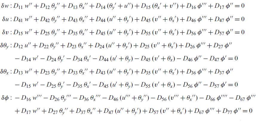
The following boundary conditions are enforced to solve the coupled homogeneous system of equations at
 $ x = 0$
and
$ x = 0$
and
 $ x = L$
:
$ x = L$
:
 \begin{align} & u(0) = u_1\quad v(x) = v_1\quad w(0) = w_1\quad \theta_x(0) = \theta_{x1}\quad \theta_{y1}(0) = \theta_{y} \quad \phi(0) = \phi_1 \nonumber\\[3pt] & u(L) = u_2\quad v(L) = v_2 \quad w(L) = w_2 \quad \theta_x(L) = \theta_{x2} \quad \theta_y(L) = \theta_{y} \quad \phi(L) = \phi_2 \end{align}
The six governing equations, along with the boundary conditions, are solved analytically to obtain the exact solution of the displacement fields in Maple(26). In the current model, each displacement field in a two-node beam element depends on all 12 Degrees of Freedom (DOF) [
 $ w_1, \, v_1, \, u_1, \, \phi_1, \, \theta_{x1}, \, \theta_{y1}, \, w_2, \, v_2, \, u_2, \, \phi_2, \, \theta_{x2}, \, \theta_{y2}$
]. This means that the interdependence of the displacement fields is taken into account. The coefficients in the polynomial are functions of the material and cross-section properties. The obtained displacement field will serve as the shape functions in the finite element formulation.
$ w_1, \, v_1, \, u_1, \, \phi_1, \, \theta_{x1}, \, \theta_{y1}, \, w_2, \, v_2, \, u_2, \, \phi_2, \, \theta_{x2}, \, \theta_{y2}$
]. This means that the interdependence of the displacement fields is taken into account. The coefficients in the polynomial are functions of the material and cross-section properties. The obtained displacement field will serve as the shape functions in the finite element formulation.
The information about the shape functions and kinematics relationship is quantified in the matrix B in the finite element formulations. The matrix B is calculated from the shape functions obtained from Equation (16) and generalised strains as follows:
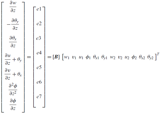 \begin{equation}\begin{bmatrix} \dfrac{\partial w}{\partial z} \\[15pt] - \dfrac{\partial \theta_y}{\partial z} \\[15pt] \dfrac{\partial \theta_x}{\partial z} \\[15pt] \dfrac{\partial u}{\partial z} + \theta_y \\[10pt] \dfrac{\partial v}{\partial z} + \theta_x \\[10pt] \dfrac{\partial^2 \phi}{\partial z^2}\\[10pt] \dfrac{\partial \phi}{\partial z}\\[10pt] \end{bmatrix} = \begin{bmatrix} e1 \\[15pt] e2 \\[15pt] e3 \, \, \\[15pt] e4 \, \\[15pt] e5 \, \\[15pt] e6\\[15pt] e7\\[15pt]\end{bmatrix} = [\textbf{\textit{B}}] \, \begin{bmatrix} w_1 \, \, v_1 \, \, u_1 \, \, \phi_1 \, \, \theta_{x1} \, \, \theta_{y1} \, \, w_2 \, \, v_2\, \, u_2 \, \, \phi_2 \, \, \theta_{x2} \, \, \theta_{y2}\, \, \end{bmatrix}^T\end{equation}
where the matrix B is defined as
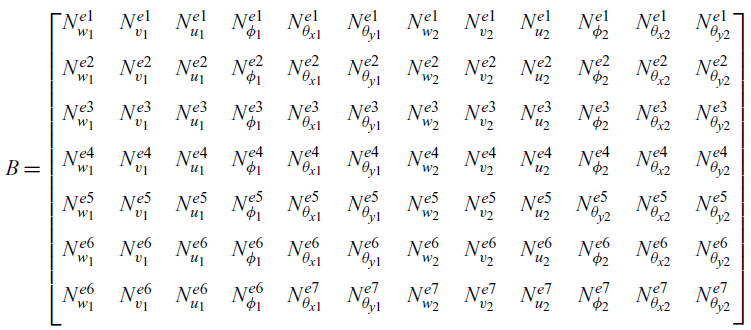 \begin{equation} B = \left[\begin{array}{@{}c@{\quad}c@{\quad}c@{\quad}c@{\quad}c@{\quad}c@{\quad}c@{\quad}c@{\quad}c@{\quad}c@{\quad}c@{\quad}c@{}} N^{e1}_{w_1} & N^{e1}_{v_1} & N^{e1}_{u_1} & N^{e1}_{\phi_1} & N^{e1}_{\theta_{x1}} & N^{e1}_{\theta_{y1}} & N^{e1}_{w_2} & N^{e1}_{v_2} & N^{e1}_{u_2} & N^{e1}_{\phi_2} & N^{e1}_{\theta_{x2}}& N^{e1}_{\theta_{y2}}\\ \\[-6pt] N^{e2}_{w_1} & N^{e2}_{v_1} & N^{e2}_{u_1} & N^{e2}_{\phi_1} & N^{e2}_{\theta_{x1}} & N^{e2}_{\theta_{y1}} & N^{e2}_{w_2} & N^{e2}_{v_2} & N^{e2}_{u_2} & N^{e2}_{\phi_{2}} & N^{e2}_{\theta_{x2}}& N^{e2}_{\theta_{y2}}\\ \\[-6pt] N^{e3}_{w_1} & N^{e3}_{v_1} & N^{e3}_{u_1} & N^{e3}_{\phi_1} & N^{e3}_{\theta_{x1}} & N^{e3}_{\theta_{y1}} & N^{e3}_{w_2} & N^{e3}_{v_2} & N^{e3}_{u_2} & N^{e3}_{\phi_2} & N^{e3}_{\theta_{x2}}& N^{e3}_{\theta_{y2}}\\ \\[-6pt] N^{e4}_{w_1} & N^{e4}_{v_1} & N^{e4}_{u_1} & N^{e4}_{\phi_1} & N^{e4}_{\theta_{x1}} & N^{e4}_{\theta_{y1}} & N^{e4}_{w_2} & N^{e4}_{v_2} & N^{e4}_{u_2} & N^{e4}_{\phi_2} & N^{e4}_{\theta_{x2}}& N^{e4}_{\theta_{y2}}\\ \\[-6pt] N^{e5}_{w_1} & N^{e5}_{v_1} & N^{e5}_{u_1} & N^{e5}_{\phi_1} & N^{e5}_{\theta_{x1}} & N^{e5}_{\theta_{y1}} & N^{e5}_{w_2} & N^{e5}_{v_2} & N^{e5}_{u_2} & N^{e5}_{\theta_{y2}} & N^{e5}_{\theta_{x2}}& N^{e5}_{\theta_{y2}}\\ \\[-6pt] N^{e6}_{w_1} & N^{e6}_{v_1} & N^{e6}_{u_1} & N^{e6}_{\phi_1} & N^{e6}_{\theta_{x1}} & N^{e6}_{\theta_{y1}} & N^{e6}_{w_2} & N^{e6}_{v_2} & N^{e6}_{u_2} & N^{e6}_{\phi_2} & N^{e6}_{\theta_{x2}}& N^{e6}_{\theta_{y2}}\\ \\[-6pt] N^{e6}_{w_1} & N^{e6}_{v_1} & N^{e6}_{u_1} & N^{e6}_{\phi_1} & N^{e7}_{\theta_{x1}} & N^{e7}_{\theta_{y1}} & N^{e7}_{w_2} & N^{e7}_{v_2} & N^{e7}_{u_2} & N^{e7}_{\phi_2} & N^{e7}_{\theta_{x2}}& N^{e7}_{\theta_{y2}}\\ \\[-6pt] \end{array}\right]\end{equation}
where
 $ N^{e1}_{u_1} $
denotes the coefficient of
$ N^{e1}_{u_1} $
denotes the coefficient of
 $u_1$
in the expression of e1.
$u_1$
in the expression of e1.
Using Equations (13) and (19), the element stiffness matrix is calculated as
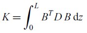 \begin{equation} K = \int_{0}^{L} B^T D \, B \, \mathrm{d}z\end{equation}
The element stiffness matrix K is obtained using analytical integration in Maple. Note that such an analytical approach enables the analytical calculation of the sensitivities of the stiffness matrix K with respect to the material stiffness matrix D. These sensitivities are of critical importance for efficient gradient-based optimisation of thin-walled composite structures.
4.1 Beam model as a design tool
The laminated composite beam model developed in this study is intended to be used as a design optimisation tool for a laminated composite thin-walled composite beam. The design variable can be the fibre directions in the plies and cross-sectional shape parametric variables. This is facilitated by the fact that the material stiffness matrix (commonly known as the cross-section stiffness matrix)
 $\textbf{\textit{D}}$
is merely a symbolic variable in the analytical integration of the stiffness matrix
$\textbf{\textit{D}}$
is merely a symbolic variable in the analytical integration of the stiffness matrix
 $\textbf{\textit{K}}$
given by Equation (20). For a particular cross-sectional geometry and ply layups, the matrix
$\textbf{\textit{K}}$
given by Equation (20). For a particular cross-sectional geometry and ply layups, the matrix
 $\textbf{\textit{D}}$
can be calculated numerically using Equation (21) (see Appendix). Thus, the analytical stiffness matrix calculation is a one-time cost, and the cross-sectional stiffness matrix can be easily evaluated repetitively for different geometry and ply layups.
$\textbf{\textit{D}}$
can be calculated numerically using Equation (21) (see Appendix). Thus, the analytical stiffness matrix calculation is a one-time cost, and the cross-sectional stiffness matrix can be easily evaluated repetitively for different geometry and ply layups.
5.0 RESULTS
Non-classical couplings of composite laminated box beams are analysed for three different types of orthotropic layup. These include the circumferentially asymmetric stiffness (CAS) configuration, the circumferentially uniform configuration (CUS) and the cross-ply layup configuration(Reference Rehfield, Atilgan and Hodges4). The ply angle orientations for the CUS and CAS configurations are shown in Fig. 2. Table 1 lists the ply orientation in each wall of the box beam for different configurations. The material properties and ply layup are listed in Table 2. The beam span and cross-sectional dimensions of the box beam are listed in Table 3. The results and convergence studies are carried out with one end of the beam fixed and the other end subjected to shear force or torque (i.e. fixed-free BC with loading at the free end). These boundary conditions are chosen to verify the developed beam model against experimental results available in literature.
Table 1 Box beam layup configurations
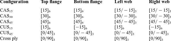
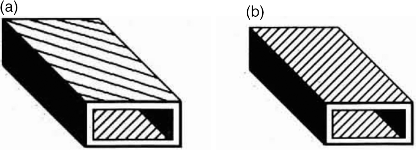
Figure 2. Ply orientations in box beam: (a) CUS configuration. (b) CAS configuration.(Reference Smith and Chopra5)
5.1 Super-convergence of the beam model
The shape functions of the beam element are exact solutions of the homogeneous Euler–Lagrangian equations listed in Equation (16). Therefore, the beam element converges to the solution in just one element, which shows the super-convergent property of the developed beam element. Figure 3 shows the convergence of the bending slope under a tip shear load of 1lb for different numbers of beam elements. The tip bending slope obtained using the present model is normalised by the tip bending slope obtained by the experiment carried by Smith et al.(Reference Smith and Chopra5).
Table 2 Material properties of AS4/3501-6 graphite–epoxy
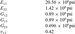
Table 3 Beam geometry for different configurations
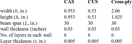
Figure 3. Convergence of the beam model – CAS
 $_{30}$
configuration.
$_{30}$
configuration.
5.2 CAS configuration
The CAS configuration exhibits bending–torsion and extension–shear coupling. Therefore, the application of a bending load results in coupled twisting. The beam twist obtained by the present model is compared with the experiments and analysis studied by Smith et al.(Reference Smith and Chopra5) in the refined 3D model developed by Stemple and Lee(Reference Stemple and Lee7).
Figure 4(a), (b) and (c) shows a comparison of the spanwise twist angle of the beam subjected to a 1lb tip shear load. The results are generally in good agreement with the experimental data.
Figure 5 shows the bending slope of the beam under 1lb shear load. The obtained results are in good agreement with the literature results. The beam twist under 1in. lb tip torque is shown in Fig. 6. The results show excellent agreement with the experimental data.
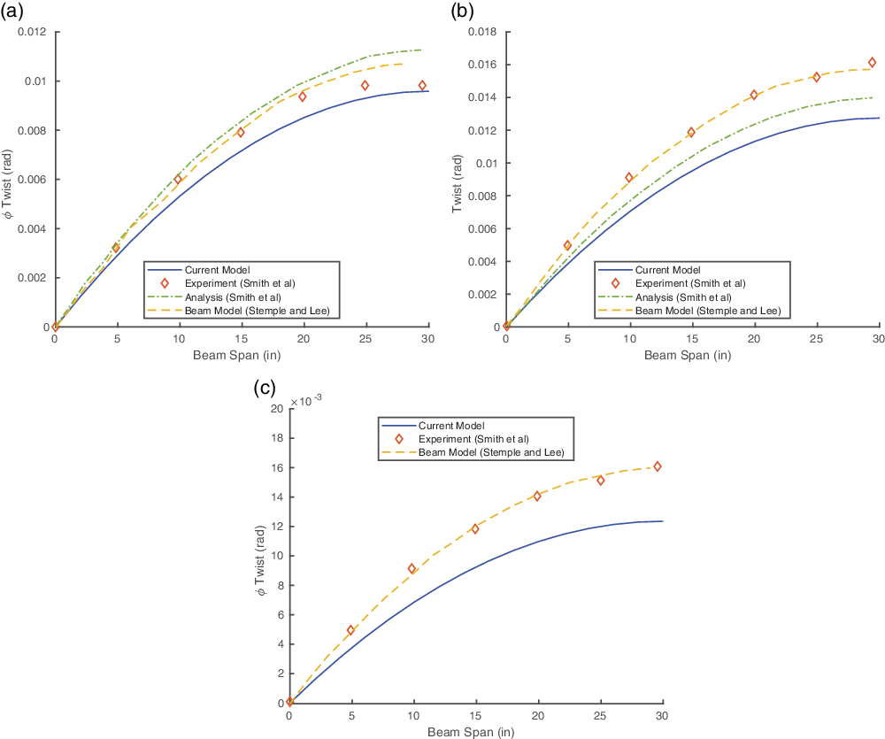
Figure 4. Twist angle for the CAS configuration under 1lb tip shear load. (a) CAS
 $_{15}$
configuration. (b) CAS
$_{15}$
configuration. (b) CAS
 $_{30}$
configuration. (c) CAS
$_{30}$
configuration. (c) CAS
 $_{45}$
configuration.
$_{45}$
configuration.
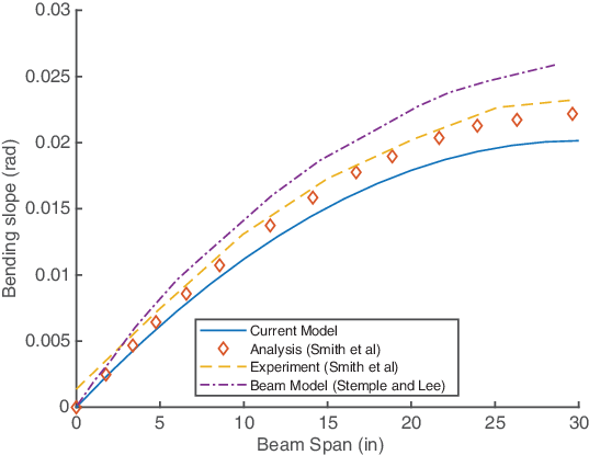
Figure 5. Bending slope for the CAS
 $_{30}$
configuration under 1lb tip shear load.
$_{30}$
configuration under 1lb tip shear load.
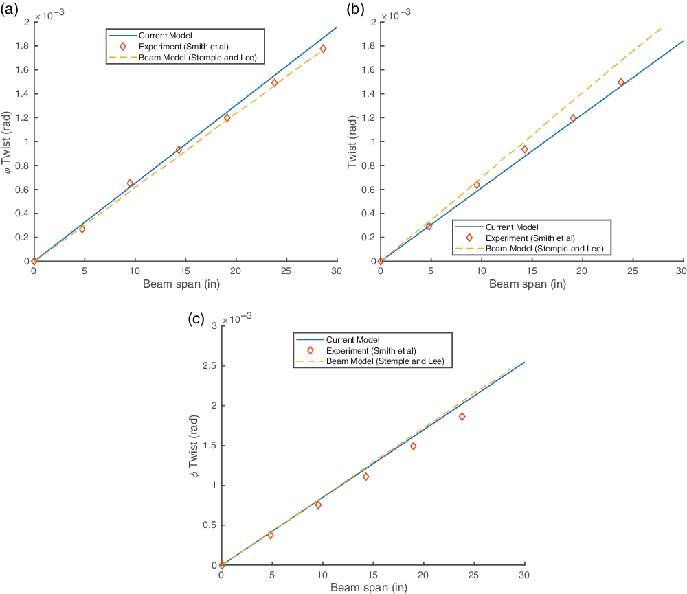
Figure 6. Twist angle for the CAS configuration under 1in.-lb tip torque. (a) CAS
 $_{45}$
configuration. (b) CAS
$_{45}$
configuration. (b) CAS
 $_{30}$
configuration. (c) CAS
$_{30}$
configuration. (c) CAS
 $_{15}$
configuration.
$_{15}$
configuration.
Table 4 CAS – configuration: quantitative comparison of tip twist (rad) under 1lb shear and 1in.-lb torque

Table 4 compares the tip twist obtained using the current approach with that of the 3D refined beam model by Stemple and Lee(Reference Stemple and Lee7) and the experimental values obtained by Smith et al.(Reference Smith and Chopra5). The present model shows a maximum error comparable to that of the beam model by Stemple and Lee (Reference Stemple and Lee7).
5.3 CUS configuration
The CUS configuration in the box beam results in extensional–twist coupling. The coupled beam extension and twisting are generated by the applied torque. The CUS configuration has been studied for two configurations:
 $\text{CUS}_{15}$
and
$\text{CUS}_{15}$
and
 $\text{CUS}_{45}$
under torque and shear loading.
$\text{CUS}_{45}$
under torque and shear loading.
Figure 7(a) and (b) shows the bending slope under 1lb shear load. The bending slope predicted by the current model is in good agreement with experiment and the analytical results by Smith et al.(Reference Smith and Chopra5). Note that, in both experiments, non-zero bending slope exists at the root. The reason for this behaviour can be attributed to the large bending–traverse shear coupling effects inherent in CUS configurations (Reference Smith and Chopra5).
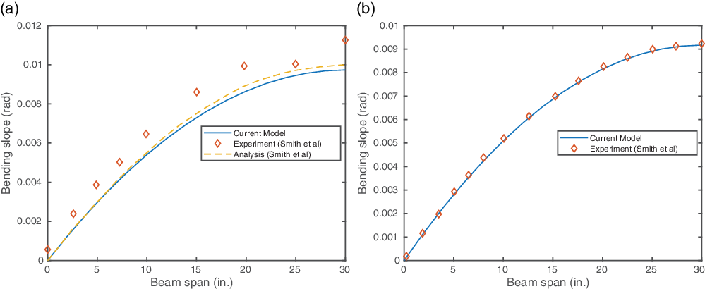
Figure 7. CUS configuration results under 1lb tip shear load. (a) CUS
 $_{15}$
configuration. (b) CUS
$_{15}$
configuration. (b) CUS
 $_{45}$
configuration.
$_{45}$
configuration.
The 1in.-lb tip torsion induced twist is shown in Fig. 8(a) and (b). Similar to the other configurations, the twist varies linearly along the beam span. The obtained results are validated by comparison with the experimental results by Chandra et al.(Reference Chandra and Chopra11).
Tables 5 and 6 list the tip bending slope and twist for shear and torque loading, respectively. The error obtained using the current approach is comparable to that obtained by Kim and White (Reference Kim and White27).
Table 5 CUS – Configuration: Quantitative comparison of tip bending slope (rad) under the 1lb tip load
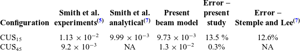
Table 6 CUS – configuration quantitative comparison of tip bending slope (rad) under 1in.-lb torque load
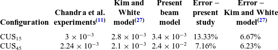
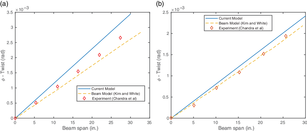
Figure 8. CUS configuration results under 1in.-lb tip torque load. (a) CUS
 $_{15}$
configuration. (b) CUS
$_{15}$
configuration. (b) CUS
 $_{45}$
configuration.
$_{45}$
configuration.
5.4 Cross-ply configuration
Figure 9(a) shows the spanwise twist angle for the beam under 1in.-lb torque. Since the cross-ply configuration exhibits no elastic coupling, there is no coupled displacement of the beam associated with the tip torque. Figure 9(b) shows the spanwise bending slope for 1lb tip shear load. Similar to the toque loading, there is no coupled displacement associated with the shear loading. The numerical results obtained are in good agreement with the experiments.
Table 7 presents a comparison of the error obtained by the present study and Kim and White(Reference Kim and White27). In comparison with the Kim and White(Reference Kim and White27) beam model, the present model predicts the deflection to a fair degree of accuracy, as is evident from the percentage error.
Table 7 Cross-ply configuration: quantitative comparison tip bending slope and twist
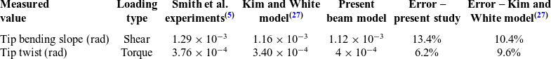
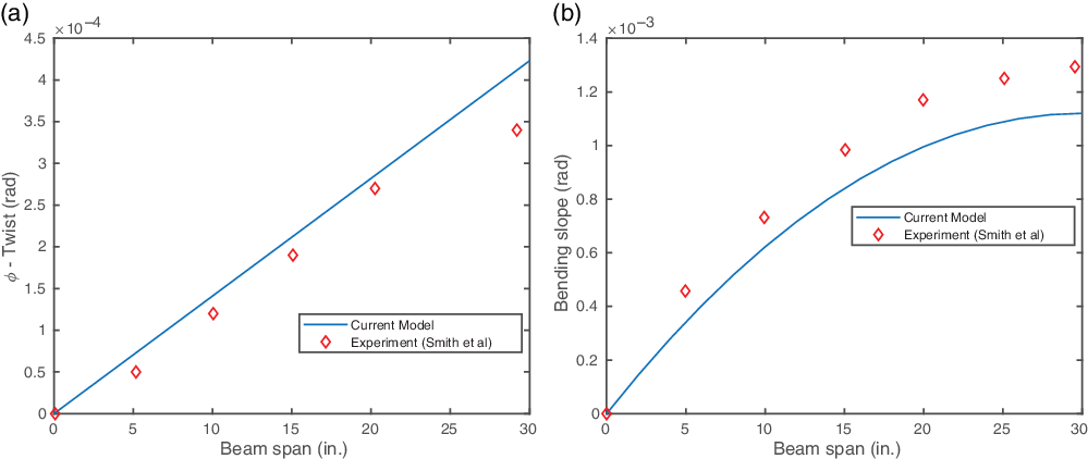
Figure 9. Cross-ply configuration results. (a) Twist angle for under 1in.-lb tip torque load. (b) Bending slope under 1lb tip shear load.
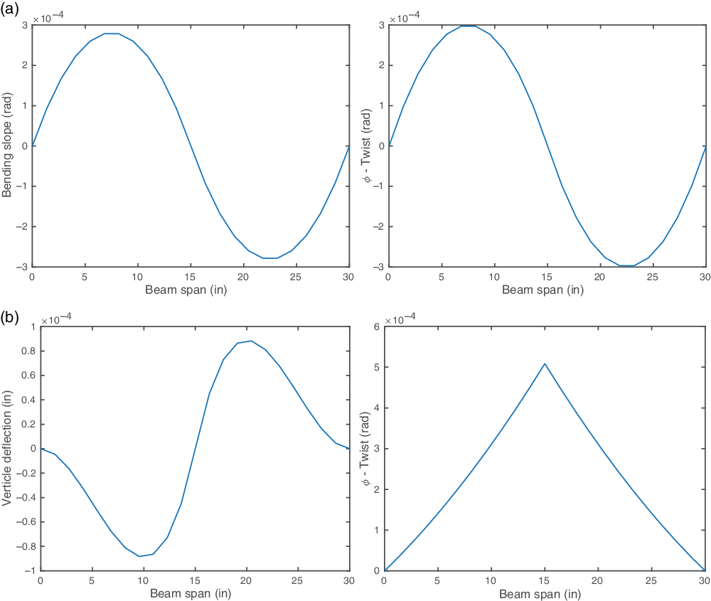
Figure 10.
 $\text{CAS}_{15}$
configuration results with fixed–fixed boundary condition and mid-span point load/torque. (a) Bending slope and twist for mid-span 1lb shear load. (b) Vertical displacement and twist for mid-span 1in.-lb torque load.
$\text{CAS}_{15}$
configuration results with fixed–fixed boundary condition and mid-span point load/torque. (a) Bending slope and twist for mid-span 1lb shear load. (b) Vertical displacement and twist for mid-span 1in.-lb torque load.
5.5 Numerical results for beam with mid-span point loading
In the previous sections, a fixed–free (fixed at one end and free at the other end) beam with a shear/torque load at the free end was considered. In this section, a fixed–fixed (both ends of the beam fixed) beam with a point load/torque at the mid-span is considered. The beam dimensions and material properties are listed in Tables 3 and 2, respectively. For the sake of brevity, only CAS
 $ _{15}$
, CUS
$ _{15}$
, CUS
 $ _{45}$
and cross-ply configuration results are studied.
$ _{45}$
and cross-ply configuration results are studied.
Figure 10(a) shows the span-wise distribution of the bending slope and twist. As expected, the beam exhibits the bending–torsion coupling inherent to the CAS configuration. Figure 10(b) shows the span-wise vertical deflection and twist under the mid-span 1in.-lb torque loading.
Figures 11 and 12 shows the mid-span loading results for the CUS
 $_{45}$
and cross-ply configurations. The twist along the beam-span varies linearly with change in slope at the mid-span. As expected, the cross-ply configuration does not exhibit elastic coupling under shear or torque.
$_{45}$
and cross-ply configurations. The twist along the beam-span varies linearly with change in slope at the mid-span. As expected, the cross-ply configuration does not exhibit elastic coupling under shear or torque.
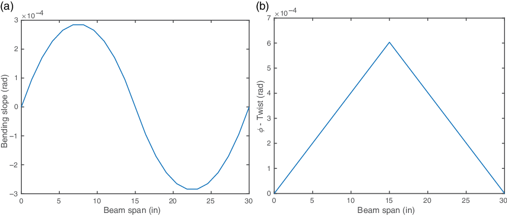
Figure 11.
 $\text{CUS}_{45}$
configuration results with fixed–fixed boundary condition and mid-span point load/torque. (a) Bending slope for mid-span 1lb shear load. (b) Twist for mid-span 1in.-lb torque load.
$\text{CUS}_{45}$
configuration results with fixed–fixed boundary condition and mid-span point load/torque. (a) Bending slope for mid-span 1lb shear load. (b) Twist for mid-span 1in.-lb torque load.
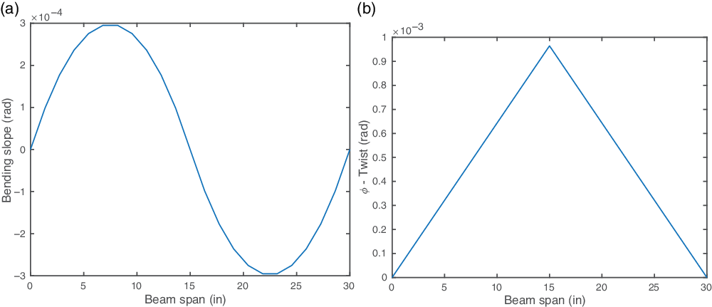
Figure 12. Cross-ply configuration results with fixed–fixed boundary condition and mid-span point load/torque. (a) Bending slope for mid-span 1lb shear load. (b) Twist for mid-span 1in.-lb torque load.
6.0 CONCLUSION
A super-convergent beam element with arbitrary cross-section is developed for the analysis of laminated composite thin-walled structures. The shape functions of the element are constructed from the analytical solutions to the homogeneous Euler–Lagrangian equations. As a result, the exact stiffness matrix is obtained for the laminated composite thin-walled beams. The developed beam model includes elastic couplings which can be exploited to enhance the response behaviour of the structure. Numerical results show that the developed element is accurate and correctly predicts the elastic coupled deformations.
In the present work, the shape functions and stiffness matrix are derived analytically using Maple. Moreover, the derivatives can also be obtained by symbolic analysis. Consequently, implementation of AD is not required for gradient-based numerical optimisation involving thin-walled composite laminated structures. The next step of this research could be the optimisation of such structures. Owing to the methodology implemented in the present work, the computational cost and development time for an optimisation framework will be greatly reduced. These effects would be even more pronounced in coupled aero-structural optimisation of composite lifting surfaces.
A APPENDIX
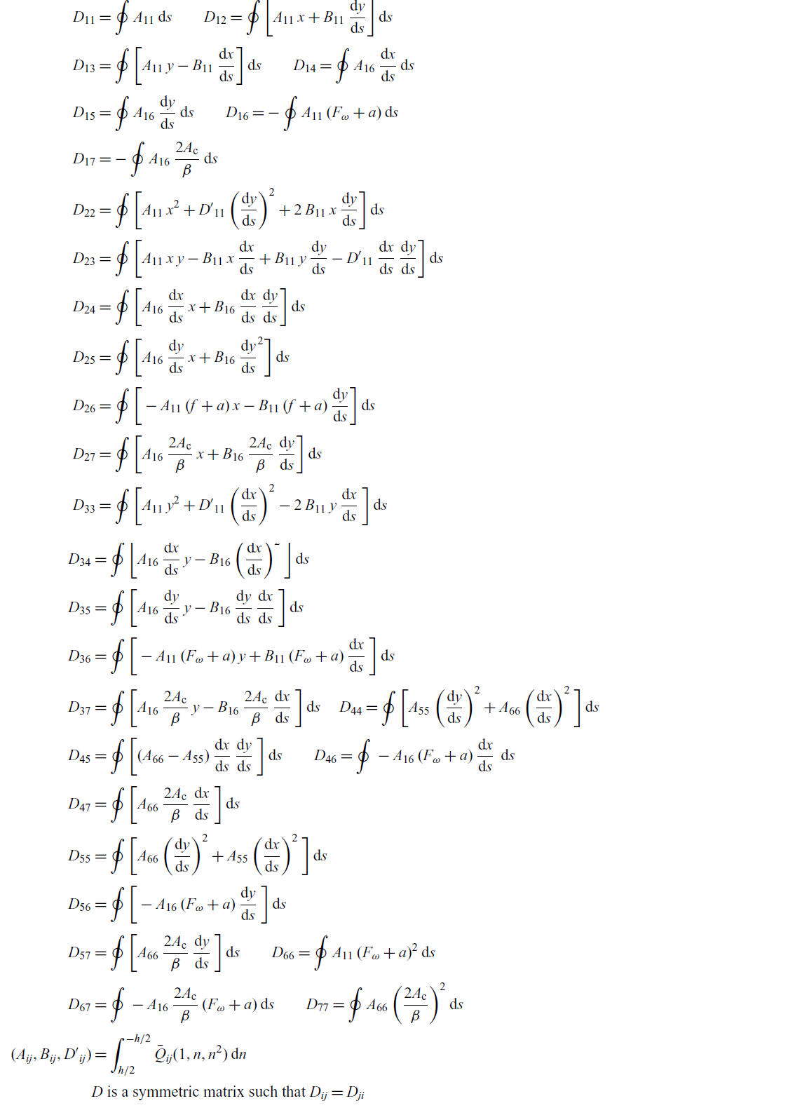 \begin{align} D_{11} &= \oint{} {A}_{11}\, \mathrm{d}s \qquad D_{12} = \oint{} \bigg[{A}_{11} \, x + {B}_{11} \, \dfrac{\mathrm{d}y}{\mathrm{d}s}\bigg] \,\mathrm{d}s \, \nonumber\\[3pt] D_{13} &= \oint{} \bigg[{A}_{11} \, y - {B}_{11} \, \dfrac{\mathrm{d}x}{\mathrm{d}s}\bigg] \,\mathrm{d}s \qquad D_{14} = \oint{} {A}_{16} \, \dfrac{\mathrm{d}x}{\mathrm{d}s}\,\mathrm{d}s \, \nonumber\\[3pt] D_{15} &= \oint{} {A}_{16} \, \dfrac{\mathrm{d}y}{\mathrm{d}s}\,\mathrm{d}s \qquad D_{16} = - \oint{} {A}_{11} \, (F_\omega + a)\,\mathrm{d}s \, \nonumber\\[3pt] D_{17} &= - \oint{} {A}_{16} \, \dfrac{2 A_{\rm c}}{\beta} \,\mathrm{d}s \, \nonumber\\[3pt] D_{22} &= \oint{} \bigg[ A_{11} \, x^2 + D'_{11} \, \bigg(\dfrac{\mathrm{d}y}{\mathrm{d}s}\bigg)^2 + 2 \, B_{11} \, x \, \dfrac{\mathrm{d}y}{\mathrm{d}s} \bigg] \, \mathrm{d}s \, \nonumber\\[3pt] D_{23} &= \oint{} \bigg[A_{11} \, x \, y - B_{11} \, x \, \dfrac{\mathrm{d}x}{\mathrm{d}s} + B_{11} \, y \, \dfrac{\mathrm{d}y}{\mathrm{d}s} - D'_{11} \, \dfrac{\mathrm{d}x}{\mathrm{d}s} \, \dfrac{\mathrm{d}y}{\mathrm{d}s}\bigg] \, \mathrm{d}s \, \nonumber\\[3pt] D_{24} &= \oint{} \bigg[ A_{16} \, \dfrac{\mathrm{d}x}{\mathrm{d}s} \, x + B_{16} \, \dfrac{\mathrm{d}x}{\mathrm{d}s} \, \dfrac{\mathrm{d}y}{\mathrm{d}s}\bigg] \, \mathrm{d}s \, \nonumber\\[3pt] D_{25} &= \oint{} \bigg[ A_{16} \, \dfrac{\mathrm{d}y}{\mathrm{d}s} \, x + B_{16} \, \dfrac{\mathrm{d}y}{\mathrm{d}s}^2\bigg] \, \mathrm{d}s \, \nonumber\\[3pt] D_{26} &= \oint{} \bigg[-A_{11} \, ( f + a) \, x - B_{11} \, (f + a) \, \dfrac{\mathrm{d}y}{\mathrm{d}s}\bigg] \, \mathrm{d}s \,\nonumber\\[3pt] D_{27} &= \oint{} \bigg[A_{16} \, \dfrac{2 A_{\rm c}}{\beta} \, x + B_{16} \, \dfrac{2 A_{\rm c}}{\beta} \, \dfrac{\mathrm{d}y}{\mathrm{d}s}\bigg] \, \mathrm{d}s \,\nonumber\\[3pt] D_{33} &= \oint{} \bigg[ A_{11} \, y^2 + D'_{11} \, \bigg(\dfrac{\mathrm{d}x}{\mathrm{d}s}\bigg)^2 - 2 \, B_{11} \, y \, \dfrac{\mathrm{d}x}{\mathrm{d}s} \, \bigg] \, \mathrm{d}s \, \nonumber\\[3pt] D_{34} &= \oint{} \bigg[ A_{16} \, \dfrac{\mathrm{d}x}{\mathrm{d}s} \, y - B_{16} \, \bigg(\dfrac{\mathrm{d}x}{\mathrm{d}s}\bigg) ^2 \, \bigg] \, \mathrm{d}s \, \nonumber\\[3pt] D_{35} &= \oint{} \bigg[ A_{16} \, \dfrac{\mathrm{d}y}{\mathrm{d}s} \, y - B_{16} \, \dfrac{\mathrm{d}y}{\mathrm{d}s}\, \dfrac{\mathrm{d}x}{\mathrm{d}s} \, \bigg] \, \mathrm{d}s \, \nonumber\\[3pt] D_{36} &= \oint{} \bigg[ -A_{11} \, ( F_\omega + a) \, y + B_{11} \, (F_\omega + a) \, \dfrac{\mathrm{d}x}{\mathrm{d}s} \, \bigg] \, \mathrm{d}s \, \nonumber\\[3pt] D_{37} &= \oint{} \bigg[A_{16} \, \dfrac{2 A_{\rm c}}{\beta} \, y - B_{16} \, \dfrac{2 A_{\rm c}}{\beta} \, \dfrac{\mathrm{d}x}{\mathrm{d}s}\,\bigg] \, \mathrm{d}s \quad\, D_{44} = \oint{} \bigg[A_{55} \ \bigg(\dfrac{\mathrm{d}y}{\mathrm{d}s}\bigg)^2 + A_{66} \, \bigg(\dfrac{\mathrm{d}x}{\mathrm{d}s}\bigg)^2 \,\bigg] \, \mathrm{d}s \, \nonumber\\[3pt] D_{45} &= \oint{} \bigg[(A_{66} - A_{55}) \, \dfrac{\mathrm{d}x}{\mathrm{d}s} \, \dfrac{\mathrm{d}y}{\mathrm{d}s}\, \bigg] \, \mathrm{d}s \qquad D_{46} = \oint{} - A_{16} \, (F_\omega + a) \, \dfrac{\mathrm{d}x}{\mathrm{d}s} \, \, \mathrm{d}s \, \nonumber\\[3pt] D_{47} &= \oint{} \bigg[A_{66} \, \dfrac{2 A_{\rm c}}{\beta} \, \dfrac{\mathrm{d}x}{\mathrm{d}s} \, \bigg] \, \mathrm{d}s \, \nonumber\\[3pt] D_{55} &= \oint{} \bigg[A_{66} \, \bigg(\dfrac{\mathrm{d}y}{\mathrm{d}s}\bigg)^2 + A_{55} \, \bigg(\dfrac{\mathrm{d}x}{\mathrm{d}s}\bigg)^2 \, \bigg] \, \mathrm{d}s \, \nonumber\\[3pt] D_{56} &= \oint{}\bigg[ - A_{16} \, (F_\omega + a) \, \dfrac{\mathrm{d}y}{\mathrm{d}s} \, \bigg] \, \mathrm{d}s \, \nonumber\\[3pt] D_{57} &= \oint{}\bigg[A_{66} \, \dfrac{2 A_{\rm c}}{\beta} \, \dfrac{\mathrm{d}y}{\mathrm{d}s}\, \bigg] \, \mathrm{d}s \qquad D_{66 }= \oint{} A_{11} \, ( F_\omega + a)^2\, \mathrm{d}s \, \nonumber\\[3pt] D_{67} &= \oint{} -A_{16} \, \dfrac{2 A_{\rm c}}{\beta} \, (F_\omega +a) \, \mathrm{d}s \qquad D_{77} = \oint{}A_{66} \,\bigg( \dfrac{2 A_{\rm c}}{\beta}\bigg)^2\, \mathrm{d}s \, \nonumber\\[3pt] (A_{ij}, B_{ij}, D'_{ij}) &= \int_{h/2}^{-h/2} \bar{Q}_{ij}(1,n,n^2) \,\mathrm{d}n \nonumber\\[3pt] &\text{\textit{D} is a symmetric matrix such that $ D_{ij} = D_{ji}$} \end{align}


 Open access