


1. Introduction
The aspect ratio of the Last Glacial Maximum (LGM) Laurentide ice sheet, as represented by the ICE-4G reconstruction of Reference PeltierPeltier (1994, Reference Peltier1996, Reference Peltier1998a), presents a challenge to coupled-climate three-dimensional (3–D) thermomechanical ice-sheet models (ISMs) of the last glacial cycle. In order to reproduce both the low surface elevation of the central dome of the ICE-4G model at LGM, required to deliver the observed southward extent of the margin, and to match the LGM Laurentide ice volume, coupled-climate and 3–D ISMs (Reference Huybrechts and TsiobbelHuybrechts and T’Siobbel, 1995,Reference Huybrechts and T’siobbel1997; Reference Tarasov and PeltierTarasov and Peltier, 1999) have required an enhancement factor for the flow law 20 to 30 times that required to reproduce the present-day Greenland ice sheet, based on transient model simulations. Furthermore, in the coupled 3–D thermomechanical ISM and the two-dimensional energy-balance-climate model (EBM) of Reference Tarasov and PeltierTarasov and Peltier (1999), near complete deglaciation of a full glacial cycle was also found to require the same very significant "speed-up" of the flow law. There is no physical process known to account for this discrepancy in the rheologies required to understand the large-scale continental ice sheets.
In one attempt to identify candidate mechanisms, Reference Marshall, Tarasov, Clarke and PeltierMarshall and others (in press) investigated a number of poorly constrained glacial processes with respect to their ability to allow the ice-dynamics model to reproduce the thin low-sloping Laurentide ice sheet of the IGE-4G reconstruction. Marine-based ice dynamics and calving were found to have a possibly significant impact on certain aspects of ice-sheet evolution, such as ice-sheet mobility and divide structure. However, the conclusion based upon these analyses was that these mechanisms were unable to account for the differences in the required flow-law enhancement. Mechanisms not ruled out included widespread basal flows and paleoclimate-ice-sheet fluctuations that could produce LGM ice sheets that were far from equilibrium.
Reference Marshall, Clarke, Dyke and FisherMarshall and others (1996) carried out a discriminant analysis of a host of North American geological and topographic properties in order to map ice-bed coupling strengths for North America. They found high support for fast basal flows over the Great Plains, continental shelf, much of the Great Lakes region and the area west of Hudson Bay. Fast basal flows over these regions would certainly impact the Laurentide ice sheet. Furthermore, steady-state flowline reconstructions with widespread basal flows over the sediment-covered regions of Hudson Bay and the southern Laurentide have yielded ice complexes in close agreement with the IGE-4G reconstruction (Reference Clark, Licciardi, MacAyeal and JensonClark and others, 1996). However, the assumptions that both the ice sheets and climate state were in equilibrium together with the external "fixing" of the ice-sheet margin suggests that these simple flowline-based reconstructions cannot be construed to have delivered definitive insight.
Due to the computational resources required to integrate them, all coupled-climate-ISM modeling studies of the 100 000 year glacial cycle must rely on highly reduced climate models and/or forcings. Given the uncertainties still present even in state-of-the-art general circulation models (GCMs), it is clear that the climate components of coupled glacial-cycle models cannot themselves be ruled out as possible explanations for the "aspect-ratio problem". Climate fields exert their influence on the cryosphere most strongly through their impact on surface mass balance (Reference Tarasov and PeltierTarasov and Peltier, 1997a). Therefore uncertainties in climate translate into uncertainties in surface mass balance.
In the present paper, three possible explanations for the discrepancy in required flow enhancement between the Greenland and Laurentide ice sheets will be investigated and evaluated. These include: enhanced basal flows; alterations to the time dependence of surface mass balance; and alterations to the spatial pattern of surface mass balance.
2. Model Description
Our coupled model is composed of a non-linear energy-balance-climate model (EBM) (Reference Deblonde, Peltier and HydeDeblonde and others, 1992), a simple isostatic-adjustment model to describe the viscoelastic relaxation of the surface under the weight of the ice, a positive degree-day (PDD) model to determine ice-surface ablation, and a 3–D thermomechanical ISM coupled implicitly to a bed-thermal model. Aside from the EBM, all components of the model are computed on a 1° longitude by 0.5° latitude grid. Model simulations are run over the entire last glacial cycle from the Eemean interglacial at 122 kyr before present (hereafter BP) with the annual cycle of sea-level temperature computed from the EBM every 500 years. Both the Eurasian and North American ice-sheet complexes are explicitly predicted while the climate and sea-level impacts of the Greenland and Antarctic ice sheets are parameterized on account of their relatively fixed margins. The ice-dynamics and isostatic-adjustment models are modified versions of those presented in Reference Deblonde and PeltierDeblonde and Peltier (1991, Reference Deblonde and Peltier1993) while the mass-balance and ice and bed thermodynamic components are fully detailed in Reference Tarasov and PeltierTarasov and Peltier (1997b, Reference Tarasov and Peltier1999). For the sake of clarity, a brief overview of these components follows.
2.1. Climate and surface mass balance
The EBM climate model is a non-linear version of the original two-dimensional EBM of Reference North, Mengel and ShortNorth and others (1983) which computes a full seasonal cycle with albedo feedback. It has been validated against the predictions of coarse-resolution GGMs under LGM boundary conditions for large spatial scales in the extra-tropics (Reference Hyde, Crowley, Kim and NorthHyde and others, 1989). The EBM derives sea-level temperature from the radiative energy balance of each tropospheric and mixed-layer ocean column using a spherical harmonic representation truncated at degree and order 11 according to the following evolution equation:

The absorbed short-wave insolation is given by the product of the solar constant, Q, the solar distribution function, S/4 and the effective co-albedo a(r,l) which tracks the seasonal variation of snow and sea-ice lines. Longwave emission is represented by a linear function of sea-level temperature derived from satellite observations, [A + BT(r,l)]. Horizontal transport is modeled as a diffusion process, with diffusion coefficient D tuned to preserve the present-day observed mean meridional temperature gradient. The heat capacity, C, is a function of surface type, but does not take into account seasonal variations. The model also incorporates a parameterized time-dependent North Atlantic heat flux (NAHF) and takes into account the radiative forcing of varying atmospheric PC02 by assuming the Vostok chronology applies globally (Reference Barnola, Raynaud, Korotkevich and LoriusBarnola and others, 1987; Reference JouzelJouzel and others, 1987).
Given that the strength of energy-balance models is their ability to capture the impact of radiative perturbations on surface-sea-level temperature, the raw output of the EBM is not directly coupled to the ISM. Rather the EBM is employed to compute perturbations to a present-day observational climatology (based upon a 14 year mean (1982–95) of re-analyzed European Center for Medium-range Weather Forecasts monthly mean-temperature fields, ds090.0 NMG/ NGAR global re-analysis project dataset). Adjustments from sea level to surface temperature are carried out by assuming a fixed 7.5°C km−1 environmental lapse rate.
The ablation model uses the now standard PDD formalism (Reference ReehReeh, 1991) with ablation parameters, unless otherwise stated for specific model runs, of 3 and 8 mm/PDD of ice equivalent for snow and ice respectively. Furthermore, 60% of melted snow is assumed to refreeze to superimposed ice. Monthly PDD are computed from monthly mean temperatures with a normal statistical model using a standard deviation of 5.5° G.
Calving represents an important component of ice-sheet mass balance, however given the small-scale controls and complexities of this process, no credible model is available, especially on "whole-ice-sheet" scales. Therefore, for the sake of simplicity, we assume that complete calving of ice occurs at the 400 m bathymetric contour.
Given its dependence on small-scale atmospheric dynamics, precipitation is much more difficult to constrain in reduced models. In the work performed to date, we have simply chosen to perturb a present-day monthly precipitation climatology (Reference Legates and WillmottLegates and Willmott, 1990) by a 3% reduction per degree cooling of gridpoint monthly mean sea-level temperature with respect to the present, in weak correspondence with the effect expected as a consequence of the temperature dependence of saturation vapour pressure. Furthermore an added desert-elevation effect (Reference Budd and SmithBudd and Smith, 1981) is also incorporated, whereby precipitation is decreased by 50% for each kilometer by which the surface elevation exceeds the height of 2 km. Rain/snow fractions are computed using a normal statistical model with a standard deviation of 4.5°C based on monthly mean temperatures, again using the logic of the PDD formalism.
2.2. Ice and bed dynamics and thermodynamics
The initial bedrock topography is derived from the ETOP05 dataset using a 2:1 weighted average of the mean and maximum gridcell elevations to capture the high-elevation nucleation zones better. Deformation of the bedrock is computed on the assumption that it occurs via a simple, local, damped return to isostatic equilibrium with an e-folding time of 4 kyr.
The 3–D thermomechanical ISM incorporates full coupling between an ISM based on Glen’s flow law and an ice-thermodynamics solver. The ice dynamics assumes the Arrhenius-type temperature dependence discussed fully in Reference PatersonPaterson (1994). The evolution equation for the ice thickness, H, is based on the vertically integrated continuity equation for ice mass as:

in which horizontal ice velocities, ![]() are determined in the shallow-ice approximation by the expression (Reference HutterHutter,1983):
are determined in the shallow-ice approximation by the expression (Reference HutterHutter,1983):

Here h is the ice-surface elevation above present-day sea level, P i is the density of ice, g is the acceleration due to gravity, T* is the ice temperature relative to the pressure-melting point and G is the mass balance. In the Glen rheology, the stress exponent n is set to 3.
According to Reference WeertmanWeertman’s (1957) original analysis, basal sliding would be expected to be controlled by a combination of two mechanisms, namely ice deformation and regelation (pressure-melting and refreezing). However, as argued by Reference PatersonPaterson (1994), it is expected that ice deformation should predominate for large-scale ice sheets (or at least for numerical models thereof). As such, the sliding law for the basal velocity of a large-scale ice sheet would be expected to be of the form:
wherever the base is at or near the pressure-melting point. This form obviously avoids the issue of hydrological controls for which no credible large-scale model presently exists. As a reference model, we have chosen to employ a simple Weertman sliding model validated for simulations of the Greenland ice sheet (Reference HuybrechtsHuybrechts, 1996), with A, = 2 × 10⁻¹³ Pa−3 m a"1.
The temperature field for the ice sheet is computed on the basis of an evolution equation for the internal energy that incorporates the influence of both horizontal and vertical advection, vertical diffusion (with temperature-dependent diffusion coefficient k(T)), and heat generation due both to ice deformation, Qd, and sliding (incorporated as a basal-boundary condition). The evolution equation for the internal temperature of the ice is therefore:

As is common in models such as this, horizontal diffusion is not included on account of the dominant influence of horizontal advection. The thermodynamic solver employs 35 equidistant vertical layers and is implicitly coupled to a local-bed-thermal model with five layers spanning the top 2 km of the bedrock. The lower boundary condition for the bed-thermal model is assumed to be provided by the digitized geothermal heat-flux map of Reference Pollack, Hurter and JohnsonPollack and others (1993), unless otherwise stated.
2.3. Model certainties and uncertainties
In considering the properties of this coupled model, it is worthwhile to clarify which components are well-constrained and which are not. The thermomechanical ISM, with only weak reliance on the basal-sliding component, has been validated in detail in the context of the European Ice Sheet Modelling Initiative (EISMINT) model-inter-comparison project (Payne and others, 1999; Ritz and others, in preparation). Analyses of the predictions made with the models demonstrated close agreement in predicted ice-sheet topographies. It should be noted that all these models were based on the same rheology and temperature dependence of the flow law. The simple relaxation model used to represent glacial-isostatic adjustment has also been validated (Reference Tarasov and PeltierTarasov and Peltier, 1997a) against the same viscoelastic gravitationally self-consistent global model of isostatic adjustment used to compute the ICE-4G reconstruction (see, e.g., Reference PeltierPeltier (1998b) for a recent review of the required theory).
The PDD formalism, employed to compute ablation, is highly reduced. However, although there are variations in the required parameter values when the model is tuned to observations from different present-day glaciers and ice sheets (see, e.g., Reference BraithwaiteBraithwaite, 1995, Reference Braithwaite1996; Reference Jóhannesson, Sigurdsson, Laumann and KennettJohannesson and others, 1995, and references therein), this sensitivity largely translates into a freedom to tune so as to provide an adequate LGM ice volume while allowing deglaciation to obtain under appropriate conditions. It is unlikely, though unproven, that a much more detailed ablation parameterization would result in a major change in ice-sheet topography that could not be obtained through simple retuning of the PDD model.
In considering the coupled model as a whole, it is therefore clear that the climate forcing and basal components of the model are in fact the least well-constrained. The EBM is a coarse-resolution energy-balance model that neglects the influence of atmospheric dynamics. Climate forcing is most important in its impact on surface mass balance, but it also contributes the upper-boundary condition required to drive the ice-bed thermodynamics. Furthermore, the precipitation parameterization is based on a highly simplified representation of the physical dynamics. Therefore, it is possible that uncertainties in the precipitation and climate components of the coupled model could of themselves account for the different flow-law enhancements required to simulate the Greenland and Laurentide ice sheets.
Basal-boundary conditions of the ISM do represent a poorly constrained and incomplete representation of actual physical processes. Though a sliding model is incorporated, there is presently little constraint on the actual form of the sliding law. Furthermore, no account is taken of basal hydrology and differing basal-surface materials. Two other processes highly sensitive to basal hydrology, namely ice streaming and deformation of subglacial till, are also not explicitly included in the model. Both sliding and till deformation reduce coupling between bed and ice and thereby enhance ice flow.
These weak constraints on modeled climate and basal processes motivated the following investigation into the possible roles that uncertainties with respect to these processes might have in explaining the aspect-ratio challenge that the IGE-4G reconstruction presents to those who would model the evolution of continental-scale ice-age ice sheets.
3. Model Analyses
The choice of flow and sliding enhancements is difficult to constrain. Observations of borehole tilt on the Greenland ice sheet do indicate enhancements of 2–10 of Glen’s flow law for certain types of older, Wisconsinan, ice relative to newer Holocene ice (Reference Dahl-Jensen and GundestrupDahl-Jensen and Gundestrup, 1987; Reference Thorsteinsson, Waddington, Taylor, Alley and BlankenshipThorsteinsson and others, 1999). Mechanisms for this enhancement appear to include: development of anisotropic fabrics due to recrystallization of ice grains under shear (Reference Budd and JackaBudd and Jacka, 1989); and the development of smaller grain-size caused by increased dust and salt concentration in the Wisconsinan ice (Reference PatersonPaterson, 1991; Reference Thorsteinsson, Waddington, Taylor, Alley and BlankenshipThorsteinsson and others, 1999). As well, analyses with an isothermal version of our model found a somewhat reduced need for flow enhancement with increased horizontal gridpoint resolution of the ice-dynamics model (Reference Tarasov and PeltierTarasov and Peltier, 1997b). Thus some part of the required flow enhancement for simulations of both the Greenland and Laurentide ice sheets, as compared to the usual Glen flow law, are likely due to the limited gridpoint resolutions of the models. All these mechanisms add uncertainty to the actual flow parameter appropriate for numerical models. However, given the longer time-scales of the Greenland ice sheet as compared to the Laurentide ice sheet, both on account of lower mean accumulation and apparent survival through past interglacials, it is difficult to conceive how Laurentide ice could develop flow enhancements a factor 2 or more than those required for Greenland, except possibly arising from dirtier Laurentide ice (Reference PatersonPaterson, 1991, Reference Paterson1994). Therefore, as a reference limit, we have chosen a flow enhancement 2.5 times that required for our Greenland model; a factor 10 greater than the base Glen flow law used in the EISMINT intercomparison projects.
One other ice-mechanics-related mechanism not explicitly included is the impact of liquid water within the ice on effective ice viscosity Sensitivity studies for Greenland-type ice sheets found that inclusion of this polythermal mechanism resulted in a slight increase in the effective viscosity, due to a reduction in the volume of temperate ice, but no significant change in the area of temperate ice (Reference GreveGreve, 1997). Therefore, it is unlikely that this mechanism could account for the flow-enhancement discrepancy identified.
Even more difficult to constrain, given the lack of data and the complexities of basal hydrology, is the range of acceptable enhancements of the sliding law. A comparison of ice-volume chronologies (Fig. 1a) for the reference model with flow enhancement of 10, relative to the standard Glen flow law, hereafter referred to as "Tbasel0", indicates that sliding factors >1 result in less LGM ice than sliding factors ≤0.5. The comparison suggests some sensitivity with respect to sliding factors that lie between 0.5 and 1. Below this threshold, sliding has no significant impact upon the ice-volume chronology nor upon surface-elevation transects at 86.5° W (Fig. 1b), which corresponds to the longitude of maximum southerly extent of the Laurentide ice sheet for the Tbase reference model of Reference Tarasov and PeltierTarasov and Peltier (1999). All versions of Tbasel0, with sliding enhancements up to a factor of 2, exhibit minimal deglaciation, excessive dome thickness, and insufficient horizontal extent in comparison to the Tbase (80× flow and 2× sliding enhancements) model of Reference Tarasov and PeltierTarasov and Peltier (1999) and to the ICE-4G reconstruction, as is clearly demonstrated in Figure 1. Increased sliding primarily tends to decrease the southerly extent due to thinning of the margin on account of greater ice transport into the ablation zone. The base of the northern flank, and part of the core of the ice sheet, is frozen (Fig. 2b) and therefore sliding cannot act on the divide of the TbaselO model. Significant extension of the southern margin, without changes to the climate forcing, requires southward displacement of the divide to sustain surface elevations above the equilibrium-line altitude. However, given the frozen base at the current divide, southward displacement is only possible with an increase in surface elevation of the displaced divide, which is what happens when sliding enhancement is decreased from 1 to 0.5 forTbaselO.
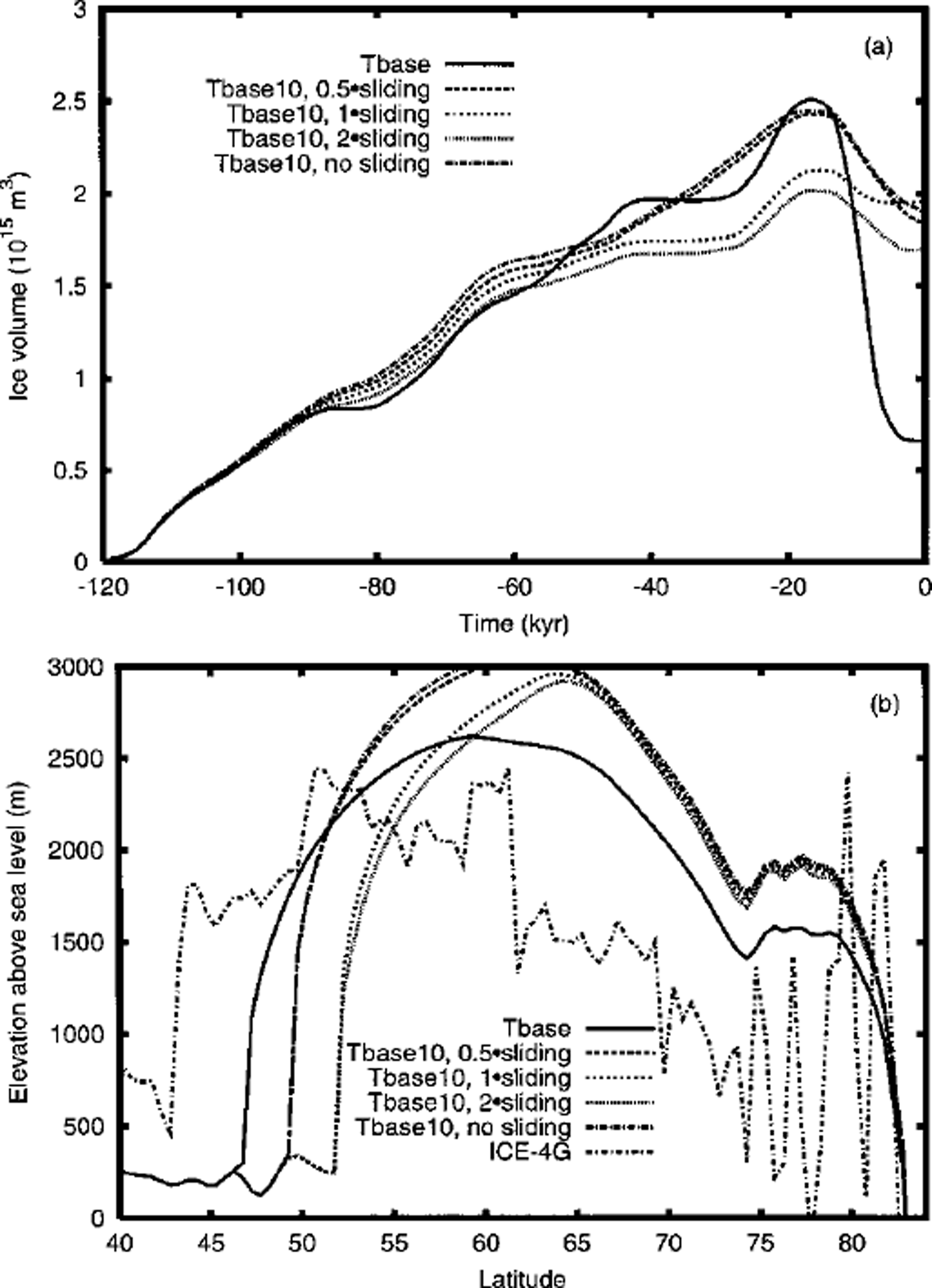
Fig. 1. Impact of different sliding enhancements to Tbasel0 model on (a) NA ice-volume chronology and (b) surface-elevation transect (also includes transect from the ICE-4G reconstruction (Reference PeltierPeltier, 1994), but does not include the contribution from "implicit ice" (Reference PeltierPeltier, 1998)). Tbasel0 uses 10 × flow enhancement of Glen flow while Tbase reference model of Reference Tarasov and PeltierTarasov and Peltier (1999) uses 80× flow enhancement and 2× sliding enhancement to Weertman sliding law as outlined in the text. Note: all transects will be taken at 86.5° W corresponding to the longitude of maximum extent for the Tbase model.

Fig. 2. Tbasel0 model with 0.5× sliding enhancement of Weertman sliding law ( Tbase uses 2× enhancement), (a) Surface topography (m) and (b) basal temperature relative to the pressure-melting point (°C).
Throughout our analyses it will be important to remember that even our Tbase reference model has insufficient southward extent compared to the geomorphologically constrained margins of the ICE-4G reconstruction (Fig. 1b). Furthermore, the apparent divide is about 3° farther south, and about a hundred or more meters lower in the ICE-4G reconstruction. The much lower surface elevations of the northern flank of ICE-4G relative to any of the Tbase and TbaselO models will be seen to be the hardest feature to obtain. This could very well be due to an error in the geophysical reconstruction in this region.
Comparison of the LGM surface topography of the TbaselO model (Fig. 2a) with 0.5 × sliding enhancement, chosen for its southerly extent, with that of the Tbase reference model reveals almost complete separation of the Cordilleran and Laurentide ice sheets, contrary to the ICE-4G reconstruction. Tbasel0 does not even extend to the Great Lakes and both southward and westward extent of the simulated Laurentide ice sheet are much short of that in the ICE-4G inference. On the other hand, Tbasel0 displays the same separation of the Innuitian dome that is characteristic of Tbase.
Comparison of the LGM basal-temperature field of the TbaselO model (Fig. 2b) with that of the Tbase model reveals a bed 1–2°C warmer on account of reduced vertical cold advection and reduced horizontal flows, allowing more time for geothermal heat to build up. Most of the Cordillera as well as much of the southern flank of the Laurentide TbaselO ice sheet have temperate bases. However, as already noted, most of the northern flank of the TbaselO Laurentide ice sheet has a frozen base.
Inspection of meridional surface- and sliding-velocity transects (Fig. 3) for the TbaselO models with various sliding enhancements reveals high maximum velocities. On this particular transect, TbaselO models have meridional surface-velocity maxima of nearly 200 m a"1 while Tbase has a maximum of over 400 m a"1 of meridional surface velocity arising only from internal ice deformation (i.e. not from sliding). However, surface velocities >100ma−1 or so, are currently observed only in ice streams and surging valley glaciers, thereby suggesting the presence of ice streams within the Laurentide ice sheet. This does raise some uncertainty with respect to the model results, given the neglect of longitudinal stresses that are known to be significant in ice streams.

Fig. 3. Impact of different sliding enhancements to Tbasel0 model on (a) meridional surface velocity (b) basal-sliding velocity.
It is noteworthy that in spite of the factor 2 range in sliding velocities, all TbaselO models have almost identical peak surface velocities for this transect. Surface velocities are of the order of balance velocities, computed as the total upstream accumulation divided by the ice thickness of the point under consideration, and decreased sliding is compensated by increased shear stress and resultant increased ice deformation. High terminal ice velocities can be expected simply on account of the large separation between divide and margin.
3.1. Impact of different sliding models
Assuming the validity of the Glen rheology, it is unlikely that the exponent in the sliding law would be below 3. However, enhancement of basal velocities through the deformation of subglacial material (Reference PatersonPaterson, 1994) is thought to have been widespread for the Laurentide ice sheet (Reference Boulton and JonesBoulton and Jones, 1979; Reference AlleyAlley, 1991) and could possibly mimic a slid-ing-law exponent as low as 1, though very large exponents approaching plastic flow have also been proposed to govern till deformation (Reference KambKamb, 1991). Lower values of the exponent in the sliding law would promote lower aspect ratios due to increased sliding away from the margins. Two simulations were carried out with linear sliding laws tuned to match the sliding velocities of the reference Weertman law for basal shear stresses of 100 kPa. As is evident from the simulated surface transects and ice-volume chronologies (Fig. 4), a sliding exponent, m, of 1 does improve both the southerly LGM extent of Tbasel0 and deglaciation, but has little impact on the elevation of the divide surface. Again, the frozen northern flank of the Laurentide ice sheet anchors the divide position and even the strongly increased sliding near the core, as compared to the exponent 3 base Weertman sliding law, associated with the 2 × enhanced linear sliding law is only able to slightly "eat away" at the divide. Stronger enhancements to the linear sliding law could have more impact on the divide. However given that the 2× enhanced linear sliding Tbasel0 model already has maximum meridional velocities of over 550 ma−1 near the margin, and maximum sliding velocities of about 300 m a−1, the numerical and physical acceptability of such enhanced and sustained large-scale flows would start to become doubtful. The surface-transect irregularities, associated with the linear sliding law, arise from finger instabilities (Payne and others, 1999) and from the transect not being along a flowline.

Fig. 4. Impact of linear-sliding model (with enhancement factors 1 and 2) applied to the Tbasel0 model on (a) NA ice-volume chronology and (b) surface-elevation transect. Tbasel0 m = 1 sliding law is tuned to match the Weertman sliding law at a basal shear stress of 100 kPa.
The improvement to Tbasel0 due to exponent 1 sliding is on the optimistic side, sliding occurs everywhere that the base is near temperate, given the lack of basal hydrology and accounting for the influence of basal-surface type. The predominance of the Canadian Shield in northern Ontario would act to reduce the area of sliding and till deformation. Furthermore, the computed basal-temperature field is quite sensitive to the geothermal heat flux, which is not strongly constrained. Use of an alternative heat-flux field based on the map of Reference Blackwell and SteeleBlackwell and Steele (1992) resulted in a decrease in the percentage area of North American ice (NA) at LGM with a temperate base from 47–34% (Reference Tarasov and PeltierTarasov and Peltier, 1999). This would have a significant impact on models relying heavily on basal processes, which all require basal temperatures to be at the pressure-melting point.
When all is taken into account, these results suggest that enhanced basal flows from low-exponent sliding, possibly due to a non Glen flow ice rheology or to extensive till deformation, can only partially improve the aspect ratio of modeled Laurentide ice sheets.
3.2. Impact of mass-balance chronology uncertainties
The largest sources of uncertainty with respect to simulated mass balance are the climate fields. Given the complexity of the climate system, it is very difficult to assign clear error bars to GCM output, let alone to the much simpler EBM and precipitation parameterizations used in the coupled model. We have therefore chosen to proceed via reducto absurdum. Instead of attempting to pinpoint error bars in the time dependence of the EBM, we have chosen two extreme glacial histories to represent strongly contrasting archetypes. These contrasting scenarios are designed to produce LGM Laurentide ice sheets that are far from equilibrium, thereby offering a limited test of the suggestion of Reference Marshall, Tarasov, Clarke and PeltierMarshall and others (in press) that paleoclimate-ice-sheet fluctuations that produce far-from-equilibrium LGM Laurentide ice sheets may be able to account for much of the required flow-law discrepancy. The first scenario, referred to as "fast growth" in Figure 5, involves suppression of Laurentian glaciation from 90–40kyrBP via an ad hoc 4°C increase of surface temperatures, as computed by the EBM, followed by a fast glaciation phase aided by an applied 4°C decrease of surface temperature from 30–25 kyr BP. This modification delivers a small improvement to both the dome elevation and the southward extent. However, the final ice volume does not differ appreciably from that of Tbasel0. Furthermore, dome peak position is not altered, thereby offering little improvement in the southward extension. An even more extreme version of this scenario ("extreme growth") with an applied 5°C warming from 90–35 kyr BP followed by an applied 5°C cooling from 33–23 kyr BP does result in major "improvements" to the Tbasel0 LGM Laurentide ice sheet. Deglaciation is slightly improved to almost 50% residual (Fig. 5a). But most significantly, the surface transect of this version of Tbasel0 is a relatively close match to that of Tbase, apart from a split divide structure, slightly lower surface elevations and about a degree of latitude less southern extent. This scenario provides an example of the impact of extreme disequilibrium.
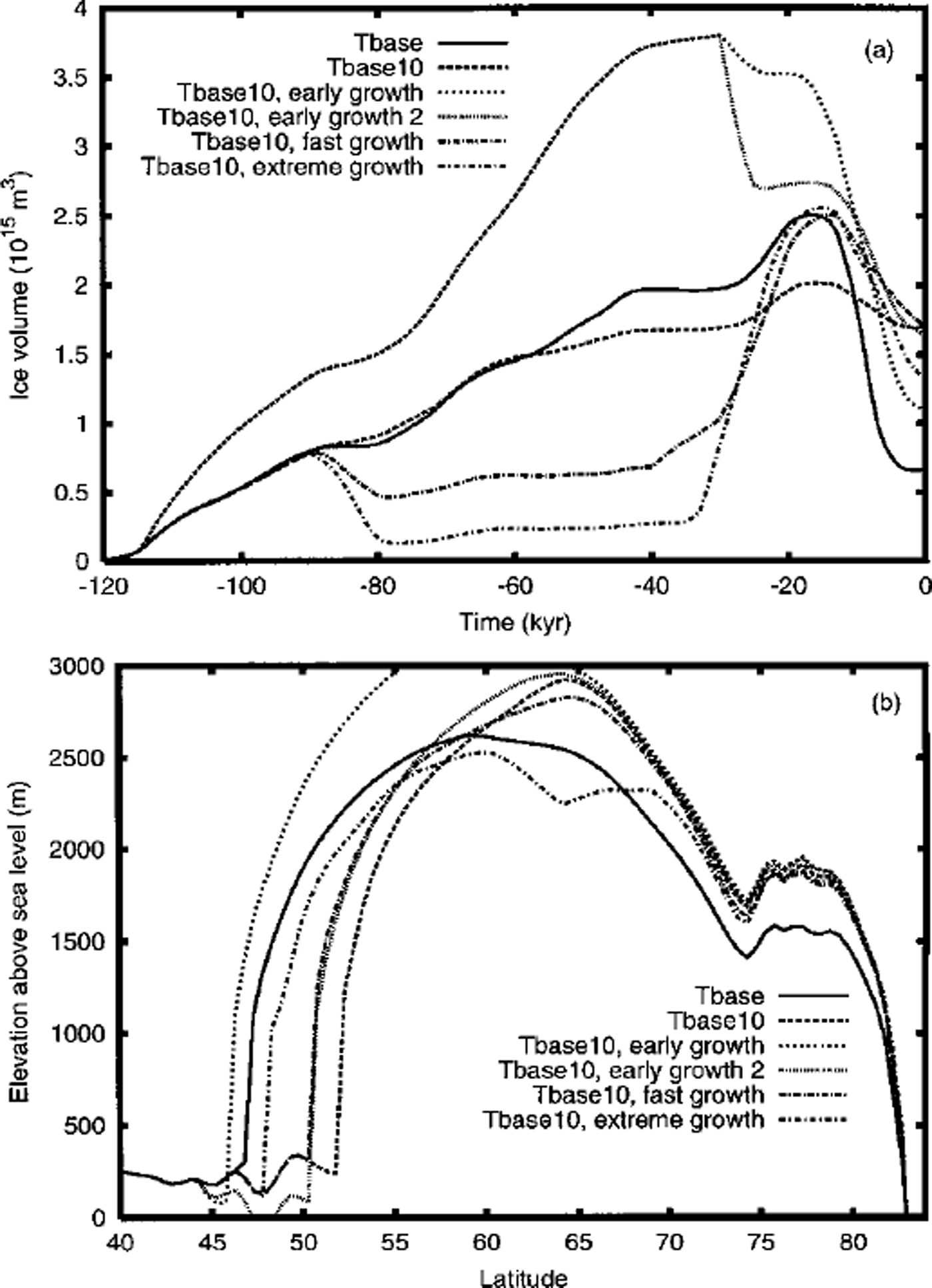
Fig. 5. Impact of different ad hoc glacial chronologies on (a) NA ice-volume chronology and (b) surface-elevation transect. The early growth model uses the Tbasel0 base model with an imposed extra TC cooling 115–35 kyr BE Early growth 2 uses same imposed cooling in addition to a 30–25kyrBP TC imposed warming. The fast-growth model uses an imposed 4°C warming from 90–40 kyr BP and an imposed 4°C cooling for 30–25 kyr BE The extreme growth model uses a 90–35 kyr BP 5° C imposed warming followed by an applied 5°C cooling for 33–23 kyr BE All models use factor 2 sliding enhancement.
The second scenario represents an opposite extreme, early glaciation aided by an applied 2°C decrease of surface temperatures 115–35 kyr BP ("early growth" in Fig. 5). This results in a large excess of ice at LGM. Application of an ad hoc 2°C increase in surface temperature from 30–25 kyr BP ("early growth 2") brings the LGM ice volume within reasonable bounds. The same small improvement to southerly extent as for the "fast growth" scenario obtains. However, in this case peak dome elevation is not lowered. It should also be stated here that such a large pre-LGM ice volume would have left a strong isostatic signature, contrary to observations.
Both of the above non-extreme scenarios produce ice-volume chronologies that (distantly) bound the range of possible NA ice-volume chronologies that could be inferred from the spectral-mapping project (SPECMAP) δ18O record of Reference Imbrie, Berger, Imbrie, Hays, Kukla and SaltzmanImbrie and others (1984) given the continental partition of ice volumes in both Tbase (Reference Tarasov and PeltierTarasov and Peltier, 1999) and the ICE-4G reconstruction. Though SPECMAP represents a filtered record of past global ice-volume changes, it is difficult to conceive how the extremely fast growth scenario could be reconciled with it. Furthermore, the large resultant isostatic disequilibrium at LGM would imply that the ICE-4G reconstruction is severely underpre-dicting LGM NA ice volume, which would likely be difficult to reconcile with the strong sea-level constraints from the Barbados coral records (Reference FairbanksFairbanks, 1989). Therefore, possible uncertainties in the time dependence of the simulated gross temperature field or mass-balance history do not appear to offer a solution to the aspect-ratio problem or required flow-enhancement discrepancy.
3.3. Impact of the geographic pattern of mass balance
Given the strong sensitivity of ice-sheet mass balance to surface temperatures on account of ablation-rate sensitivities, a trial hypothesis we wished to test is that mass-conserving changes to the geography of accumulation within the non-ablation zones of the ice sheet, the dry-snow and percolation zones, a subarea of the accumulation zone where no runoff occurs, would not have a significant impact on the ice sheet. Model simulations using Tbase parameters were carried out with mass-conserving extremal modifications to the geography of accumulation. At one extreme, the mean accumulation for the whole non-ablation zone was used at each gridpoint. The opposite extreme involved a quadratic enhancement of the meridional accumulation gradient at each longitude. Interestingly, both of these modifications resulted in a strong reduction of the degree of glaciation. To tune the modified models for a reasonable LGM ice volume, the precipitation-reduction factor (Rp) was reduced to 1% for the enhanced-accumulation-gradient scenario (Fig. 6). However, even with the elimination of the Rp (i.e. set to 0), the average-accumulation scenario produced insufficient ice volume at the LGM, slightly less than that of Tbase10 10. Furthermore, southward extent of the ice complex of this latter simulation is even less than that of Tbasel0 (Fig. 6b). Unlike most other simulations considered in this study, mean thickness chronologies for this scenario were significantly greater than those of other scenarios with even more LGM ice volume, not shown. This is the consequence of the increase of accumulation over colder regions in this scenario which allowed increased build-up of cold ice and a subsequent increase in the modeled aspect ratio.

Fig. 6. Impact of modifications to geographic pattern of accumulation on (a) NA ice-volume chronology and (b) surface-elevation transect. "Avg accum." applies non-ablation-region average accumulation to every point in that region. “Enhanced accum.” uses a mass-conserving quadratic enhancement of the accumulation gradient in the non-ablation zone. All models use factor 2 sliding enhancement and stated precipitation reduction factors Rp (default value = 3%).
The enhanced-gradient version of Tbasel0 (and Rp = 1%) leads to some improvements in the deglaciation phase of the simulation (Fig. 6a). It also leads to the southward displacement of the divide in better agreement with ICE-4G and Tbase. Most significantly, this scenario improves the aspect ratio of Tbasel0 both by decreasing divide elevation to within tens of meters of that of Tbase and by extending the southern margin beyond that of Tbase. This improvement relies on a major change in precipitation patterns with precipitation reduced by a third to a half or more north of 55° N compared to that computed for Tbase for transects at 86.5° W (not shown). Precipitation rates near the margin increase by a factor of two and surpass 1.5ma−1. This modification appears to provide one solution to the required flow-law discrepancy. However, given that Tbase already underpredicts precipitation almost everywhere over the Laurentide ice sheet, in comparison to T32 GCM simulations using ICE-4G LGM boundary conditions (Reference Vettoretti, Peltier and McFarlaneVettoretti and others, in press), there is little support for such an extreme modification.
The above results negate our trial hypothesis. Ice-sheet evolution is sensitive to the internal geography of accumulation. Given the large uncertainties with respect to GCM precipitation fields, this suggests that definitive modeling of ice sheets is dependent on accurate precipitation fields, which are difficult to obtain even with state-of-the-art GCMs.
Surface temperature is the most important control on surface mass balance, especially given the sensitivity of ablation to temperature. The margin of LGM Tbase stays between the –2.5° and –5°C mean annual isotherms along the entire southern margin. Even the reduced ice flow in Tbasel0 does not appear to hinder its southward penetration into warmer regions significantly as its southern LGM margin stays within a degree of –4°C; a result that likely would not obtain for simulations without full two-way coupling between ice and climate. Therefore, the most obvious mechanism by which we might extend the southern margin would simply be to modify the surface-temperature field.
An ad hoc cooling in the region bounded by 70°–90° W and 40°–60°N applied to the Tbase model (Reference Tarasov and PeltierTarasov and Peltier, 1999) was found to produce a southeastern lobe corresponding with the geomorphological data (Reference Dyke and PrestDyke and Prest, 1987) used to constrain the southern margin of the ICE-4G reconstruction. This result is hardly surprising given the sensitivity of surface mass balance to surface temperature. More interesting are recent analyses that suggest this imposed regional cooling may have a physical basis. GCM simulations with LGM and ICE-4G boundary conditions (Reference Vettoretti, Peltier and McFarlaneVettoretti and others, in press) produce a cooling effect in this region that is much stronger than that predicted by the EBM, even after correcting for differing surface elevations with a 7.5˚Ckml atmospheric lapse rate. This arises as a result of the strengthening of the Rossby wave field over LGM North America which results in more northerly flows over the Great Lakes region. Applying the above mentioned ad hoc cooling to Tbasel0, however, results in a large excess of LGM ice volume and high dome center. A reduction of ice volume and dome elevation, along with maintenance of the gains in southerly extent, can be obtained with an increase of the desert-elevation gradient from a two-fold to an eight-fold reduction in precipitation for every kilometer increase in surface elevation over 2 kma.s.l. However, given that the same GCM study indicates that our reference model already underpredicts precipitation almost everywhere over the Laurentide ice sheet, other mechanisms must be invoked to explain the low surface elevation of the ICE-4G Laurentide dome.
Strongly enhanced sliding with either an 8–fold sliding enhancement of the reference sliding law or use of the linear sliding law, with sliding enhancement set to 1, coupled with an extremal value for the PDD ablation parameters (4.4 and 10.0 mm/PPD of ice equivalent), allows the model to produce southward extent better than that of Tbase and within approximately two degrees of latitude of the ICE-4G margin (Fig. 7). Furthermore, deglaciation is improved significantly with the 8× reference sliding model having even less residual ice at present than Tbase, a not unexpected consequence of the increased ablation-rate parameters. However, both divide position and surface elevation remain relatively unchanged from those of Tbasel0. Though extreme, the above PDD ablation parameters cannot be ruled out on the basis of observational data (see, e.g., Reference BraithwaiteBraithwaite, 1995, Reference Braithwaite1996; Reference Jóhannesson, Sigurdsson, Laumann and KennettJohannesson and others, 1995, and references therein) especially given the uncertainties in the surface temperatures derived from an EBM based upon the assumption of a fixed lapse rate. Slight surface irregularities, situated around 55° N in the LGM-forced, lobe-enhanced, sliding-model topographies, again arise from finger instabilities and from the fact that the transect crosses different flowlines. Stronger enhancements of the sliding law (results not shown) may extend the southern margin even further (by about a half degree of latitude for 2× linear sliding), but stronger fingering instabilities along with maximum sliding velocities >350 m a"1 call into question the numerical, if not the physical, acceptability of the result. Furthermore, factor 2 sliding enhancements to the above do not significantly modify the position nor the surface elevation of the divide. This again supports the thesis that enhanced basal flows requiring a temperate base cannot extend the southern margin and significantly reduce surface elevation at the divide simultaneously, nor displace the divide southward when the northern flank has a frozen base.
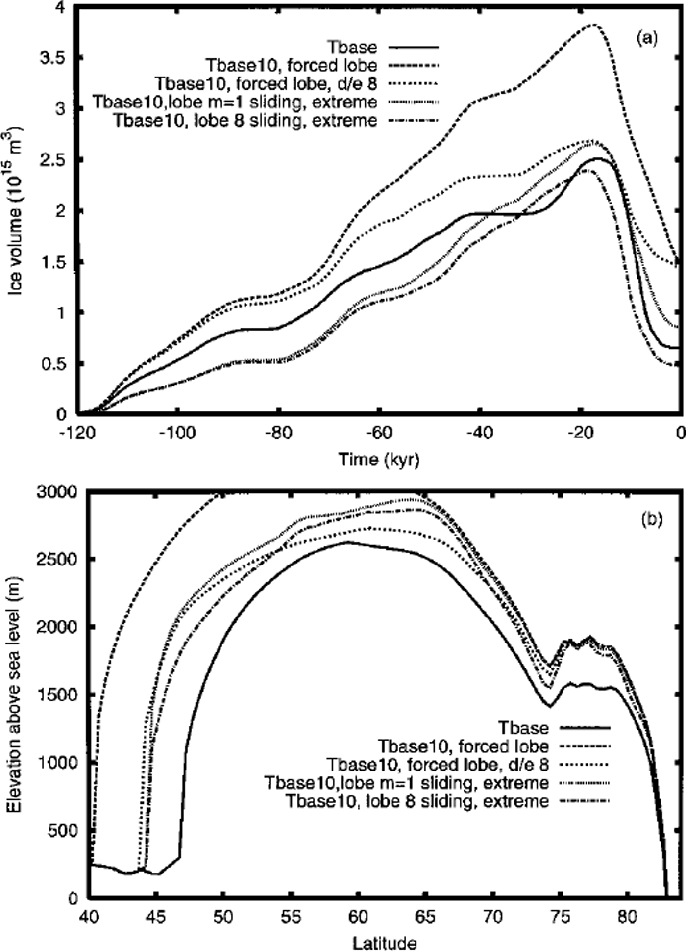
Fig. 7. Impact of ad hoc forced southeastern lobe development on (a) NA ice-volume chronology and (b) surface-elevation transect. Cooling proportional to the radiative perturbation from varying PCo2 is applied to the 90°–70° W, 60°–40° N region. "d/e8" version incorporates quartic strengthening of desert-elevation effect, "m = 1 extreme" version uses linear sliding law and 4.0 and 10.0 PPD snow and ice-melt parameters respectively. "8sliding"extreme uses identical PDD parameters but 8 × enhancement of base Weertman sliding law.
4. Conclusions
Our analysis of the ice sheets expected to form under extreme conditions has not led to the identification of a clear solution to the question of the ICE-4G aspect-ratio problem. Enhanced sliding alone contributes neither to southward extent nor to reduction of surface elevation at the divide due to the frozen northern flank of the Tbasel0 Laurentide ice sheet. Sliding laws with reduced exponents are able to increase the southward extent partly, but are unable to reduced the elevation of the dome. Given that regelation is unlikely to dominate in ice-sheet basal sliding, the use of lower-order sliding laws deliver results that are best interpreted as representing large-scale till deformation or indicating a need to modify the ice rheology itself. It should be noted that the evidence for widespread subglacial-till deformation under the Laurentide ice sheet is inconclusive (Reference AlleyAlley, 1991). Recent measurements on Ice Stream B, Antarctica, indicate that 83% of the surface motion arose within 30 mm of the ice-bed interface (Reference Engelhardt and KambEngelhardt and Kamb, 1998). These observations support the possibility of significantly enhanced sliding under large-scale ice streams or at least lend further credence to theoretical analyses suggesting that till deformation is highly non-linear (Reference KambKamb, 1991), and thereby further tend to question the physical basis for a linear sliding law.
Contrary to the results of Reference Marshall, Tarasov, Clarke and PeltierMarshall and others (in press), given the constraints of the SPECMAP record, uncertainties in the chronology of total ice-sheet mass balance do not appear to offer a solution to the aspect-ratio problem with mass-balance chronologies that produce ice sheets far from equilibrium. A strong increase of the meridional precipitation gradient was able to produce an LGM ice sheet with greater southward extent and similar surface elevation at the divide as that of Tbase. However, this modification required major reductions to precipitation rates over much of the core and all of the northern flank, contrary to the results obtained in recent analyses (Reference Vettoretti, Peltier and McFarlaneVettoretti and others, in press) in which the LGM precipitation fields of the reference coupled model are already found to be significantly lower than GCM predictions.
These analyses nevertheless highlight the sensitivity of predicted ice-sheet topography to the geographic pattern of accumulation. Even though margins are strongly controlled by surface temperatures, dome location and marginal extent are significantly influenced by the geography of the accumulation field.
Ad hoc changes to the surface-temperature field suggested by the above mentioned GCM analyses can act to form a southeastern lobe and greatly extend the southern margin. However, in order to matchTbase LGM ice volumes, strong basal sliding and extremal ablation parameters are required. Furthermore, divide surface elevations are significantly in excess of those of Tbase and the divide location is not displaced from that of Tbasel0.
The above results may be summarized as follows: enhanced basal flows can neither displace southward nor reduce the surface elevation of a divide for which the northern flank is frozen to the bed; southward displacement and simultaneous reduction in surface elevation of the divide is possible with large changes to the meridional mass-balance gradient. However these changes are contra-indicated by GCM simulations; extension of the southern margin is easily obtained with regional cooling, but in order to avoid an increase of surface elevation at the divide extreme ablation and sliding are required. Therefore, if one assumes that no more than a 2.5 flow enhancement relative to that required to simulate the Greenland ice sheet can be used for Laurentide ice sheet and if one accepts the validity of the T32 GCM simulations used to bound acceptable mass-balance changes, all of the above mechanisms and uncertainties can at best only partly account for the low surface elevation, extended margins, and southerly divide position of the ICE-4G reconstruction for the LGM Laurentide ice sheet.
It should be noted that this conclusion depends on the fact that the Tbasel0 model has a frozen base over most of its northern flank. Though this ice-sheet model has been validated against other 3–D thermomechanical ISMs for predicted surface elevations, recent model intercomparisons (Payne and others, 1999; Ritz and others, in preparation) have found significant scatter in the predicted basal-temperature fields especially when fast flows arise. Furthermore, uncertainties in the geothermal heat flux can also have a major impact on the area of temperate base. However, given that a relatively warm geothermal heat-flux map is used in the Tbasel0 model, Tbasel0 should if anything be providing a warm upper bound to the simulated Laurentide basal-temperature field.
Our analyses did not include detailed ice-stream dynamics nor did they take into consideration basal hydrology. However, by considering enhanced basal flows wherever the base was near-temperate and with maximum surface velocities in excess of 500 ma−1 arising for certain cases, and thereby approaching maximum observed velocities for large-scale ice streams (Reference ClarkeClarke, 1987), the above simulations have in effect crudely subsumed the possible impact of these processes. Analysis of transient and small-scale phenomena, such as surge lobes, would of course require detailed models of basal hydrology and ice-stream dynamics. However for the large spatial scales and millennial time-scale features under consideration here, it is unclear how the details of ice-stream dynamics and basal hydrology could act to significantly increase the further southward extent of the margins and simultaneously lower, and displace southward, ice divides which are frozen at the base of the northern flank.
One process that could reduce the thickness of ice on the northern flank would be extensive calving. However, given the shallow bathymetry of the Canadian Arctic Archipelago, it is hard to conceive of a significant reduction there. Sensitivity analyses with simple calving models can create scenarios of strongly delayed grounding of ice over Hudson Bay (Reference Marshall, Tarasov, Clarke and PeltierMarshall and others, in press). However, once grounded, the ice was found to be quite stable over Hudson Bay. Furthermore, both low- and high-calving scenarios resulted in LGM ice sheets very similar to the reference model employed for that analysis. Given the absence of a well-constrained calving model, however, it is clear that we are not yet in a position to develop any strong constraint on the role that calving might play in thinning Laurentide ice on its northern flank.
Assuming the basic validity of LGM precipitation fields predicted by the Canadian Climate Centre GCM (Reference Vettoretti, Peltier and McFarlaneVettoretti and others, in press) and with the caveat concerning the uncertain role of calving in thinning the northern flank, we are left to conclude that some major enhancement to the rate of flow of Laurentide ice is required to obtain the LGM surface topography of the ICE-4G reconstruction. This raises the question of the validity of the basic Glen flow law that is most often assumed to apply for large-scale ice-sheet modelling. The issue of alternative rheologies is addressed directly in the companion paper of Reference Peltier, Goldsby, Kohlstedt and TarasovPeltier and others (2000), a preliminary discussion having previously appeared in Reference PeltierPeltier (1998b).


