


1. Introduction
High Mountain Asia (HMA) contains the densest concentration of alpine glaciers that are sensitive to global warming. Retreat and thinning of alpine glaciers have changed meltwater flow routines and water availability thus affected daily life of the local communities (Immerzeel and others, Reference Immerzeel2020). The rapid ice mass loss has also contributed to the rise of global sea level. Glacier volume change (mass balance) due to ice thickness change and redistribution can indicate climate change directly. Therefore, it is particularly significant to study glacier mass balance across the HMA.
Glaciological in situ measurements over a limited number of glaciers and subsequent extrapolation to the entire region (WGMS, 2020) may lead to large biases toward low-altitude glaciers (Fujita and Nuimura, Reference Fujita and Nuimura2011). For the alleviation of this problem, geodetic remote-sensing datasets have been introduced to glacier mass-balance analysis to partially compensate for deficiencies of in situ measurements at high elevations. Those datasets include laser altimeter data (Kääb and others, Reference Kääb, Berthier, Nuth, Gardelle and Arnaud2012, Reference Kääb, Treichler, Nuth and Berthier2015; Wang and others, Reference Wang, Yi and Sun2021), radar altimeter data (Jakob and others, Reference Jakob, Gourmelen, Ewart and Plummer2021), Digital Elevation Models (DEMs) data (Brun and others, Reference Brun, Berthier, Wagnon, Kääb and Treichler2017; Zhou and others, Reference Zhou, Li, Li, Zhao and Ding2018; Shean and others, Reference Shean2020; Bhattacharya and others, Reference Bhattacharya2021; Hugonnet and others, Reference Hugonnet2021), the Gravity Recovery and Climate Experiment (GRACE) and GRACE-Follow On (GRACE/FO) satellites (Wouters and others, Reference Wouters, Gardner and Moholdt2019; Ciracì and others, Reference Ciracì, Velicogna and Swenson2020). Accuracy of altimeter-derived mass-balance estimates rely on representativeness of spatial sampling because only a few glaciers are sampled, and the whole glacier area is never fully sampled (Treichler and others, Reference Treichler, Kääb, Salzmann and Xu2019). DEM has advantage of high spatial resolution and temporal coverage. A time series of advanced spaceborne thermal emission and reflection radiometer (ASTER) DEMs can provide detailed glacier elevation information of each DEM pixel. Nevertheless, ASTER-derived DEM may have biased errors or voids in featureless accumulation areas (Wang and Kääb, Reference Wang and Kääb2015). Therefore, ASTER DEM stacks for a short period of time were too noisy for mass-balance estimates (Treichler and others, Reference Treichler, Kääb, Salzmann and Xu2019). Gravity is a potential field, and gravity signals can come from any changes in mass, including those from glaciers, permafrost and water storage. However, it is difficult to isolate glacier signals directly from the GRACE measurement (Zhang and others, Reference Zhang, Yao, Xie, Kang and Lei2013).
Uncertainties in glacier mass balance can be affected by penetration depth differences of different radar frequencies (Round and others, Reference Round, Leinss, Huss, Haemmig and Hajnsek2017), different spatial and temporal coverage/resolution of different data sources, as well as data accuracy. Penetration depth of radar signals through ice can be a significant source of uncertainty when using radar-based DEM data such as the C-/X-band Shuttle Radar Topography Mission (SRTM) and the updated NASADEM (NASA JPL, 2021). Radar penetration depths into glaciers can be estimated by different methods: (i) linear extrapolation of ICESat-derived glacier elevation change backdating to the SRTM acquisition date of February 2000 by assuming glacier elevation-change rate that showed the same trend during 2003–2008 and 2000–2003 (Kääb and others, Reference Kääb, Berthier, Nuth, Gardelle and Arnaud2012, Reference Kääb, Treichler, Nuth and Berthier2015); (ii) subtracting DEMs from field measurements or optical DEM (Dehecq and others, Reference Dehecq2016; Round and others, Reference Round, Leinss, Huss, Haemmig and Hajnsek2017; Lambrecht and others, Reference Lambrecht, Mayer, Wendt, Floricioiu and Völksen2018); (iii) adding the relative penetration differences between C-/X-band SRTM and the X-band penetration estimation from the assumption of dry snow percentage (Zhou and others, Reference Zhou2019); (iv) doubling the relative penetration differences between SRTM-C and X-band DEMs (Jaber and others, Reference Jaber, Rott, Floricioiu, Wuite and Miranda2019); and (v) ignoring the penetration issues by assuming that SRTM has captured the 1999 autumn elevation profiles (Berthier and others, Reference Berthier, Arnaud, Vincent and Rémy2006) and choosing data acquired during autumn season to calculate the mass balance.
ICESat-2's ATLAS instrument can provide elevation measurements with a specific timestamp and without the effect of penetration. The ICESat-2 ATL06 (Land Ice Elevation) product has been applied to study the ice mass balance of Greenland and Antarctic ice sheets (Smith and others, Reference Smith2020), small glaciers such as those in Svalbard (Sochor and others, Reference Sochor, Seehaus and Braun2021) and glacier elevation changes in steep and rugged regions such as HMA (Wang and others, Reference Wang, Yi and Sun2021; Shen and others, Reference Shen, Jia and Ren2022; Zhao and others, Reference Zhao, Long, Li, Huang and Han2022). The ICESat-2 ATL06 product was also found to have a higher accuracy than other DEM products (Chen and others, Reference Chen2022). Consequently, it is relevant to use ICESat-2 data collected over the HMA from 2018 to 2021 to study the spatiotemporal glacier mass variations. To this end, we will: (1) correct penetration depths for NASADEM to obtain penetration-corrected elevation data in 2000 by doubling the difference between the X-band SRTM DEM and NASADEM; (2) compare penetration estimations estimated with different methods; and (3) obtain the HMA glacier mass balance from 2000 to 2021 through comparing the elevation differences between ICESat-2 and penetration-corrected NASADEM.
2. Study area, data sources and methods
2.1 Study area
HMA has a glacier area of ~9.76 × 10⁴ km2 (RGI Consortium, 2017) and accounts for ~7.6% of the global glacier volume, excluding the Greenland and Antarctic ice sheets (Zemp and others, Reference Zemp2019). The climate of the HMA region is mainly controlled by three atmospheric circulation systems: the westerlies, the Indian summer monsoon (ISM) and the East Asia monsoon (Fig. 1). The climate in southern HMA is controlled by the ISM, and that in the north-western HMA is controlled by the westerlies (Ménégoz and others, Reference Ménégoz, Gallée and Jacobi2013). The climate in the south-eastern margin zones is additionally affected by the East Asia monsoon. Because of different atmospheric circulation patterns, glaciers have distinct accumulation periods and are consequently categorized into three main categories: winter-, spring- and summer-accumulated glaciers (Maussion and others, Reference Maussion2014). Different regions exhibit various percentages of debris due to local variations in geology, topographic relief and glacier dynamics (Herreid and Pellicciotti, Reference Herreid and Pellicciotti2020). Glaciers in the western and southern HMA have a high percentage of debris coverage, among which the highest occurs in the Hindu Kush mountain range (19.3%). However, glaciers in the inner HMA have a low percentage of debris coverage of about only 2% (Scherler and others, Reference Scherler, Wulf and Gorelick2018).
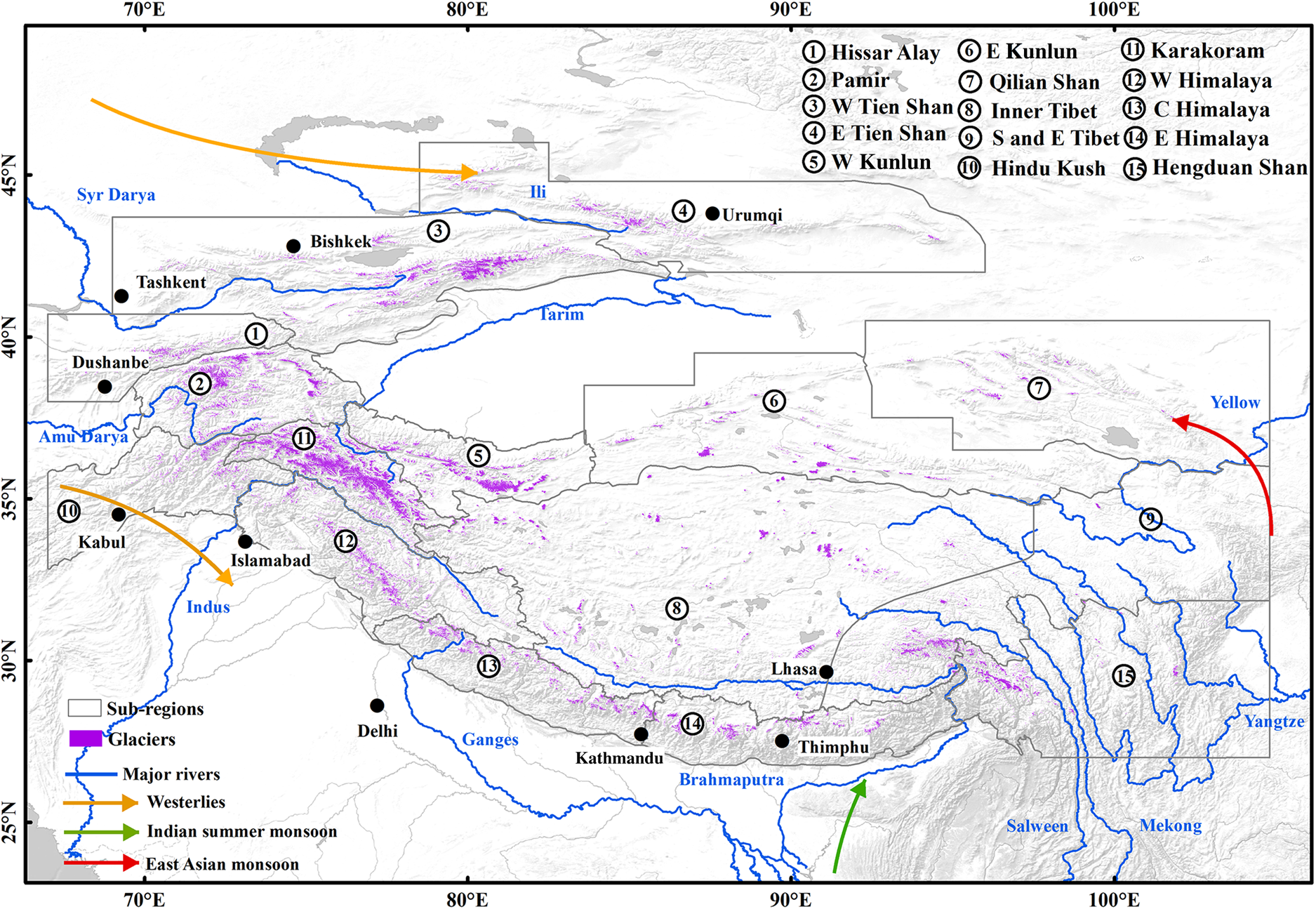
Fig. 1. Glacier distribution of the High Mountain Asia region. Purple polygons indicate glaciers, sub-region boundaries are marked and the names are notated in black. The glacier and region boundaries were from the Randolph Glacier Inventory 6.0. Blue lines and notations represent the flows and names of major HMA rivers. The arrows show the three atmospheric circulation systems of HMA, including the westerlies, Indian summer monsoon and East Asia monsoon.
2.2 Data sources
2.2.1 ICESat-2 data
The advanced topographic laser altimeter system (ATLAS) instrument on the ICESat-2 satellite provides significantly increased spatial coverage compared to previous altimeters by dividing the transmitting laser pulse into six beams (Markus and others, Reference Markus2017). The ICESat-2 ATL06 (version 4) product uses a window size ranging from 40 to 80 m to segment photons from global geo-located photon data (ATL03) to estimate the geolocated land ice surface height (Smith and others, Reference Smith2019). Pair tracks are ~3 km apart in the across-track direction, and the strong and weak beams within one pair are separated by ~90 m. Land ice surface height is then determined after corrections for instrument bias (e.g. transmit pulse shape bias correction and first-photon bias correction) (Smith and others, Reference Smith2019).
The ATL06 product contains latitude, longitude and height above the WGS84 ellipsoid for each measurement footprint. Land ice heights represent the mean surface height averaged over 40 m segments of the ground track and spaced 20 m apart (Smith and others, Reference Smith2019). ATL06 product has better than 5 cm height accuracy in the Antarctic, and the biases of two beams in one pair are <2 cm (Brunt and others, Reference Brunt, Neumann and Smith2019). Compared with in situ continuously operating reference system and unmanned aerial vehicle data acquired in Qilian Shan, ATL06 data have very high vertical and horizontal positioning accuracy (Zhang and others, Reference Zhang2021), which is indispensable for glacier mass-balance estimates.
We selected the ATLAS/ICESat-2 data that were acquired around the same season as the NASADEM was acquired (mid-February), and a window of 2 months around 15 February was chosen to obtain the appropriate laser altimetry data and minimize seasonal-related bias. Therefore, the data from 15 January to 15 March in 2019, 2020 and 2021, which included more than 2.53 × 10⁶ footprints on the glaciers over the HMA region, were used to estimate glacier mass balance.
2.2.2 DEM datasets
NASADEM is an update of the SRTM DEM. It was derived by reprocessing the original SRTM interferometric SAR data using updated interferometric unwrapping algorithms by applying vertical and tilt adjustments based upon GCPs derived from ICESat to improve the vertical accuracy (Crippen and others, Reference Crippen2016). Compared with the C-band SRTM 1 arc-second v3 product, this processing scheme can deal with strong offsets and ramps occurring in regions where the acquisition strips cross each other (Crippen and others, Reference Crippen2016). It has the best performance among the open-access DEMs (Chen and others, Reference Chen2022), and has few voids remaining. We masked out the void-fill regions in the NASADEM data (Braun and others, Reference Braun2019), as the fill-in data have a completely different time stamp and may not be inherently consistent with the original radar data on glaciers, or the data used to fill in could have already originated from optical data like ASTER Global Digital Elevation Model (GDEM) (NASA JPL, 2021).
The SRTM X-band DEM was acquired simultaneously with the NASADEM, with the same 30 m resolution; however, the SRTM-X DEM shows an ‘X’ stripe-like coverage due to a smaller swath width. The horizontal datum of the two DEM datasets is the same (WGS84 datum), but the vertical datums are different; the EGM96 geoid height datum was used for the NASADEM, and the WGS84 height datum was used for the X-band SRTM DEM. In this study, we used the X-band SRTM DEM as the reference to estimate the radar penetration depth for NASADEM.
2.2.3 Glacier boundary dataset
The Randolph Glacier Inventory (RGI) 6.0 (RGI Consortium, 2017) used images acquired near year 2000 to generate glacier boundaries all over the world. It included glaciers of all sizes, which are beneficial for glacial mass change evaluation during 2000–2021. The HMA region consists in regions 13, 14 and 15 in RGI 6.0, so we used the glacier boundaries of these three regions to classify the ICESat-2 footprints and DEM datasets into glacier and non-glacier sections.
2.3 Methods
2.3.1 Co-registration of different datasets
The EGM96 datum for the NASADEM was converted to the WGS84 height datum by adding the geoid height difference in the ENVI software. We then divided the HMA into grids of 1° × 1°, and NASADEM was registered to ICESat-2 or X-band SRTM DEM within each grid by applying the method proposed by Nuth and Kääb (Reference Nuth and Kääb2011), which is given by Eqn (1):
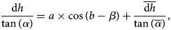
where dh is the elevation difference between the NASADEM and ICESat-2 (or X-band SRTM DEM), α is the slope, β is the aspect, a and b are the magnitude and direction of the shift vector, $\overline {{\rm d}h\;}$ is the mean elevation difference between the two DEM datasets and $\overline {\alpha \;}$
 is the mean slope.
We calculated the shift vector by applying Eqn (1) to each grid to correct the displacement. This process was iterated 30 times, and the shift vector that minimizes the product of the std dev. and the median of the elevation difference was selected as the final offset result. Each 1° × 1° NASADEM grid was shifted to the ICESat-2 data during co-registration. The detailed offset vector was shown in Figure S1. The offset in the plane was, at most, 15 m, which was less than the pixel size of the NASADEM, and the offsets in the Z direction of 99.4% (318/320) of the grids were within ±5 m.
For the NASADEM and X-band SRTM DEMs, we corrected for the maximum curvature- and elevation-dependent bias by fitting the second-order polynomial to the elevation difference on stable ground (Gardelle and others, Reference Gardelle, Berthier and Arnaud2012, Reference Gardelle, Berthier, Arnaud and Kääb2013). Filters of ±150 m in dh were used to remove outliers.
2.3.2 Representativeness of the ICESat-2 footprints
ICESat-2 samples have to match the glaciers within each spatial unit with respect to the glacier hypsometry to get a statistically robust signal (Kääb and others, Reference Kääb, Berthier, Nuth, Gardelle and Arnaud2012; Neckel and others, Reference Neckel, Kropáček, Bolch and Hochschild2014). Glacier hypsometry results of each mountain range derived from ICESat-2 and NASADEM show that there are few differences between them. But for a smaller area of interest like 1° × 1° cells, hypsometry tends to show some discrepancy. If we found that glacier hypsometry between NASADEM and ICESat-2 is larger than 10% at any elevation band for one cell, we iteratively eliminated some footprints at this elevation band until glacier hypsometry difference at all elevations is smaller than 10% (Treichler and others, Reference Treichler, Kääb, Salzmann and Xu2019; Jakob and others, Reference Jakob, Gourmelen, Ewart and Plummer2021). We generated estimates of elevation change and mass change from the reduced samples. However, if it turns out we cannot control the hypsometry difference between ICESat-2 and NASADEM under 10%, this cell would not be taken into consideration when estimating glacier mass change. In total, 256 cells were retained after this process and 46 cells were eliminated for the 1° × 1° cell mass-balance estimation. Neckel and others (Reference Neckel, Kropáček, Bolch and Hochschild2014) found that glacier elevation change became stable when the ICESat footprint ratio exceeded 60% for each mountain range. Therefore, a bootstrapping analysis was performed by iteratively and randomly selecting ICESat-2 glacier footprints and computing the mean dh value in each iteration, the sampled footprints can represent the entire region since we found the same trend for the ICESat-2 footprints.
2.3.3 Radar penetration-depth correction
The penetration depth issue of radar signals can lead to underestimation of glacier surface elevation (Kääb and others, Reference Kääb, Berthier, Nuth, Gardelle and Arnaud2012). The radar penetration depth into the snow/ice of a glacier needs to be corrected. For C-band DEM, the C-band penetration depth was corrected by doubling the difference between the X-band SRTM DEM and the NASADEM (Jaber and others, Reference Jaber, Rott, Floricioiu, Wuite and Miranda2019) using Eqn (2):

where k is the C-band penetration depth in each NASADEM elevation bin.
The coordinates of the NASADEM and X-band SRTM DEM were transformed into their corresponding UTM projections to a resolution of 30 m through cubic interpolation and then were co-registered as described in section 2.3.1. We clipped the grid by the glacier boundary of the region and analyzed the penetration depth of each sub-region according to the boundary. Penetration depths exceeding ±15 m were identified as outliers (Neelmeijer and others, Reference Neelmeijer, Motagh and Bookhagen2017). We divided each RGI mountain range into zones with 100 m intervals in elevation and calculated the median value of penetration depth in each zone, and added the value to the NASADEM value of each pixel in the corresponding bin. For areas of higher or lower elevations in which there were not enough X-band SRTM DEM pixels to be used in the penetration-depth correction, the median value of penetration depth of the nearest elevation zone was used instead.
We investigate alternative methods to estimate the penetration depth following the method proposed by Kääb and others (Reference Kääb, Berthier, Nuth, Gardelle and Arnaud2012, Reference Kääb, Treichler, Nuth and Berthier2015) for comparison of penetration estimate.
2.3.4 Mass-balance estimation
Elevation differences (dh) between the corrected NASADEM and the ICESat-2 elevation were calculated for each on-glacier footprint. The ICESat-2 footprints were enclosed according to the sub-region boundary. Any footprints with dh values exceeding ±200 m were excluded as outliers, assuming that this value was the maximum possible elevation change. First, we removed footprints using the three std dev. (3σ) outlier rejection criteria within each sub-region (Flament and Rémy, Reference Flament and Rémy2012), which removed ~5–20% footprints, with the largest removal concentrated in the southeastern HMA and the Himalaya. We then divided each sub-region into elevation zones with 100 m interval and calculated the mean dh (Ei) of each zone. If no data were available for an elevation bin, a zero elevation-change rate was assigned. Volume change was then calculated by multiplying Ei and the glacier area (Ai) of the corresponding zone. The ice density of 850 ± 60 kg m−3 was used to translate the volume change into a mass change since the ice density is appropriate for a wide range of conditions and longer-term trends (>5 years) (Huss, Reference Huss2013), and the final mass-balance change (dB) was obtained using Eqn (3):
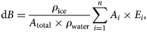
where n is the number of elevation zones, ρ ice is the glacier ice density, ρ water is the mass density of water (1000 kg m−3) (Huss, Reference Huss2013) and A total is the total glacier area in each sub-region.
2.3.5 Mass-balance accuracy assessment
Uncertainties in mass-balance estimates can originate from four sources: residual errors between ICESat-2 DEM and NASADEM after co-registration, uncertainty in penetration depth estimates, glacier area uncertainty and glacier density uncertainty.
Uncertainties of point measurements (i.e. the std dev. of the elevation based on individual grid points) were used to represent lumped uncertainty of geodetic mass balance. In that sense, the uncertainties are implied to be totally correlated (Rolstad and others, Reference Rolstad, Haug and Denby2009). Therefore, decorrelation distance has to be considered. Previous studies have assumed that the ICESat footprints within each 2 km cluster are fully correlated (Moholdt and others, Reference Moholdt, Hagen, Eiken and Schuler2010a). In case of few ICESat footprints available, a correlation distance of 5 km was chosen (Moholdt and others, Reference Moholdt, Nuth, Hagen and Kohler2010b). We used semi-variogram cloud to simulate correlation distance of ICESat-2 due to its higher resolution and denser distribution (Nuth and others, Reference Nuth, Kohler, Aas, Brandt and Hagen2007), and the value obtained was 2 km. The elevation uncertainty (σ g) that originates from the residual errors between ICESat-2 and NASADEM after co-registration was then calculated by Eqn (5):
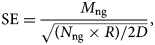
where M ng is the std dev. of the elevation differences in the non-glacier region, N ng is the number of ICESat-2 footprints in the non-glacier, R is the spatial resolution of the ATL06 product (20 m) and D is the correlation distance (2 km). SE is the standard mean error, and MD is the mean value of the elevation residuals in the non-glacier region.
The penetration correction uncertainty of the NASADEM was calculated from the std dev. of the median penetration depths for all elevation zones below 6500 m (Neelmeijer and others, Reference Neelmeijer, Motagh and Bookhagen2017). We also added the median value of penetration of the non-glacier pixels in calculating penetration correction uncertainty:
where σ penetration is the penetration correction uncertainty of the NASADEM, and ki is the median penetration depth estimated for each elevation zone in each sub-region.
The uncertainty of elevation changes in glaciers can be obtained by:
Regional mass uncertainties can be affected by uncertainty in glacier area σ A (±10%) and uncertainty in glacier density σ ice (±60 kg m−3). Uncertainty of glacier volume (σV) and mass changes (σB) will be estimated as follows:
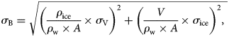
where σ V is the uncertainty in glacier volume, σ h is the uncertainty in elevation changes, A is the glacier area, σ A is the uncertainty of glacier area, dh is the mean value of glacier elevation-change rate, σ B is the uncertainty in mass change, ρ ice is the mean ice density (850 kg m−3), ρ w is the water density, V and σ V are the glacier volume change and its uncertainty, respectively.
3. Results
3.1 Penetration depths
The radar penetration depths for NASADEM DEM correction were estimated by doubling elevation difference between the X-band SRTM DEM and NASADEM DEM data. Penetration depths in the 15 sub-regions depend strongly on elevation. With increasing elevation, the radar penetration depth into snow and ice for the NASADEM showed a near linear upward trend. Exceptions occurred at the high altitudes of Hissar Alay, Central Himalaya and East Himalaya Mountains, which could be related to the uneven distribution of the X-band SRTM DEM. There were insufficient number of pixels to obtain radar penetration depth estimations at high altitudes. In general, the average penetration depths showed spatial variability in the HMA region (Fig. 2). The lowest penetration depth of ~1.00 m occurred in the South and East Tibetan Mountains, followed by that in the Hindu Kush Mountains at 1.18 m and the Karakoram Mountain at 1.78 m. The largest penetration depth occurred in the Hissar Alay and Qilian Shan mountains, while moderate penetration depths ranging from 2.26 to 4.31 m occurred in the central HMA. Most of the sub-regions exhibited a penetration depth between ±0.1 m for the off-glacier data points.
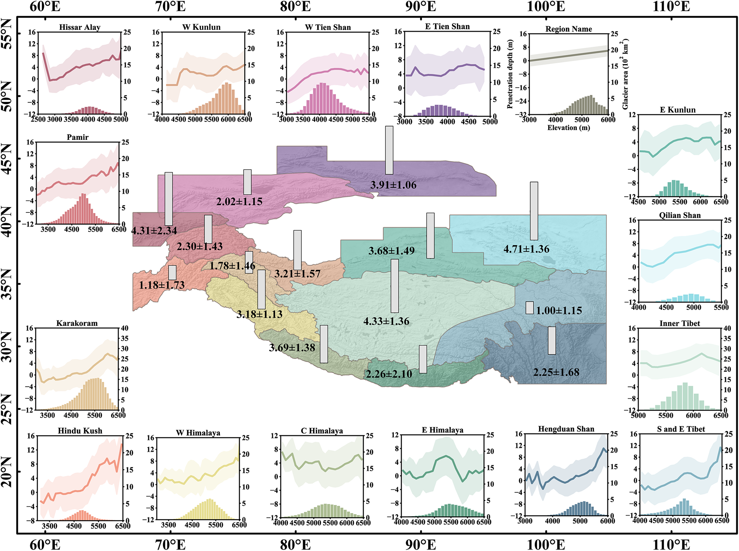
Fig. 2. NASADEM penetration of the 15 sub-regions of HMA. The bars on the spatial map show the average penetration depth of each region. The line of each subplot donates the penetration depth of each elevation bin (left y-axis), and the shade represents the penetration correction uncertainty of the corresponding bin. The horizontal lines indicate zero line to the penetration estimates. The bars of each subplot display the glacier area of the corresponding bin (right y-axis). Base map was from Esri, USGS, NOAA.
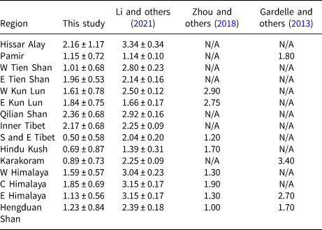
Additionally, the average penetration depths agreed well with estimations by ICESat extrapolation within the error bars in 10 of the 15 regions (Table 1). Regions with larger discrepancies concentrated in the eastern HMA, especially the South and East Tibet Mountains and the Hengduan Shan region.
Table 1. Estimated average NASADEM penetration depth (m) in this study by using method proposed by Jaber and others (Reference Jaber, Rott, Floricioiu, Wuite and Miranda2019) and comparisons with estimates based on ICESat extrapolation (error level given is 1 standard error)
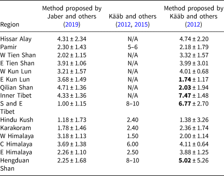
Regions with large discrepancies are marked in bold.
3.2 Altitudinal distribution of glacier elevation changes
The altitudinal distributions of the glacier elevation changes in 15 mountain ranges (sub-regions) are shown in Figure 3. The glacier elevation changes in three autumns exhibited similar patterns. For this reason, we merged data from the three years to increase data coverage and statistics. The common pattern of decreasing rates in glacier elevation with increasing altitude can be observed. All the elevation zones in the West Kun Lun Mountain showed a positive trend while thinning occurred in the Himalaya, South and East Tibet, and the Hengduan Shan Mountains, even at the highest elevations.
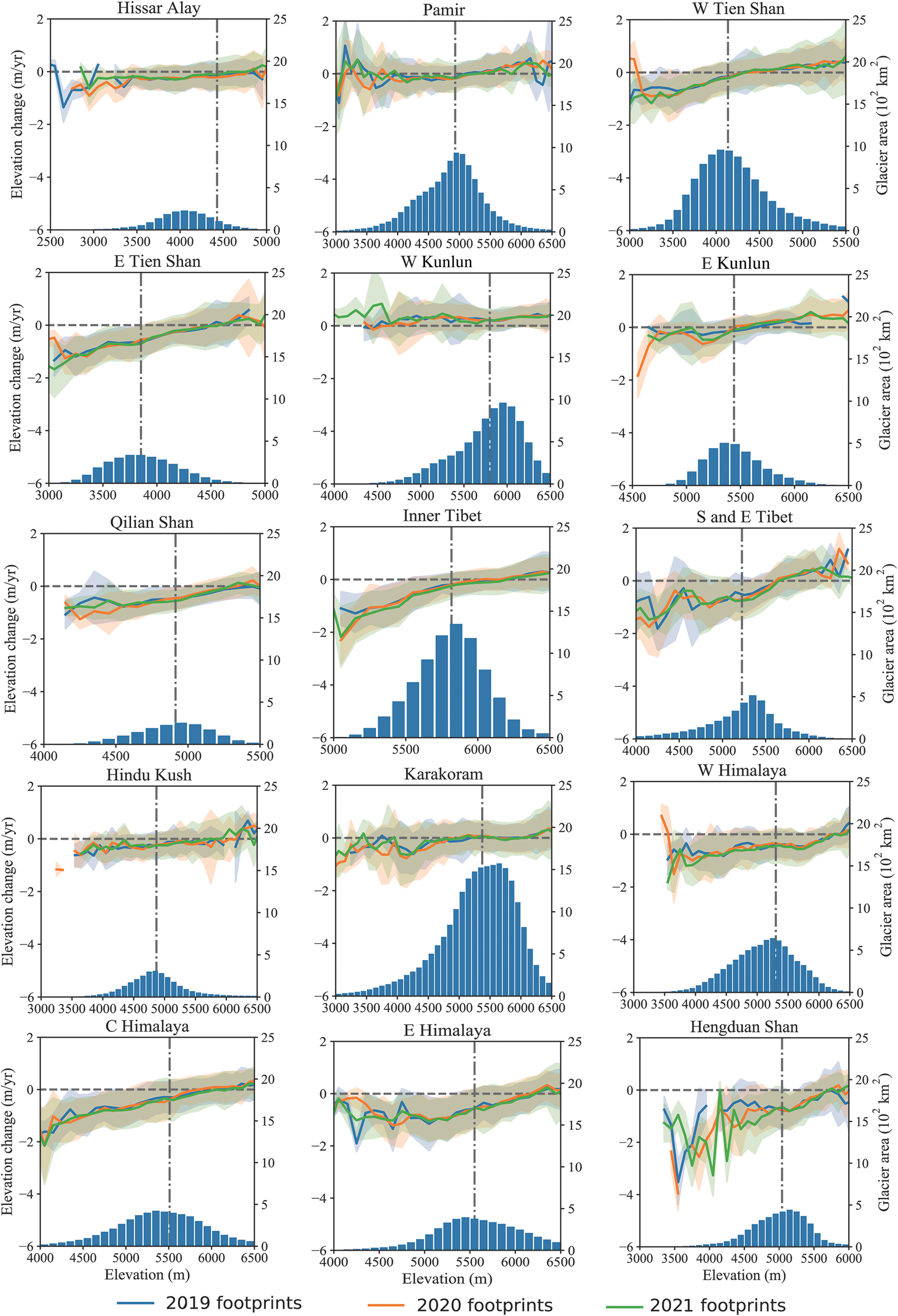
Fig. 3. Altitudinal distribution of glacier elevation changes in 15 sub-regions in HMA. The blue and orange lines represent the elevation change rates with uncertainty envelopes calculated with footprints of 2019, 2020 and 2021 for each 100 m elevation band (left y-axis). The vertical lines indicate the median glacier elevation, and the horizontal lines indicate zero line to the elevation change. The bars of each subplot display the glacier area of the corresponding bin (right y-axis).
3.3 Glacier mass-balance changes
3.3.1 Glacier mass balance of HMA mountain ranges
The estimated total mass change rate of glaciers in HMA was ~−0.18 ± 0.12 m w.e. a−1 (−17.53 ± 11.36 Gt a−1) from 2000 to 2021. Figure 4a shows the glacier mass changes per year in HMA aggregated over 1° × 1° grids in detail. The south-eastern HMA experienced a relatively significant thinning rate of up to −1 m w.e. a−1, followed by the southern and north-eastern HMA of ~−0.6 m w.e. a−1. A moderate loss rate of −0.1 m w.e. a−1 was seen in the Hissar Alay, Pamir and West Tien Shan Mountains. In contrast, a cluster of positive trends of ~0.2–0.4 m w.e. a−1 occurred near the West Kun Lun Mountains. The South and East Tibet and Hengduan Mountains exhibited the largest mass-balance uncertainty, followed by the Himalaya, while the Tien Shan, Pamirs and eastern Kun Lun Mountains were subjected to less uncertainty (Fig. 4b).
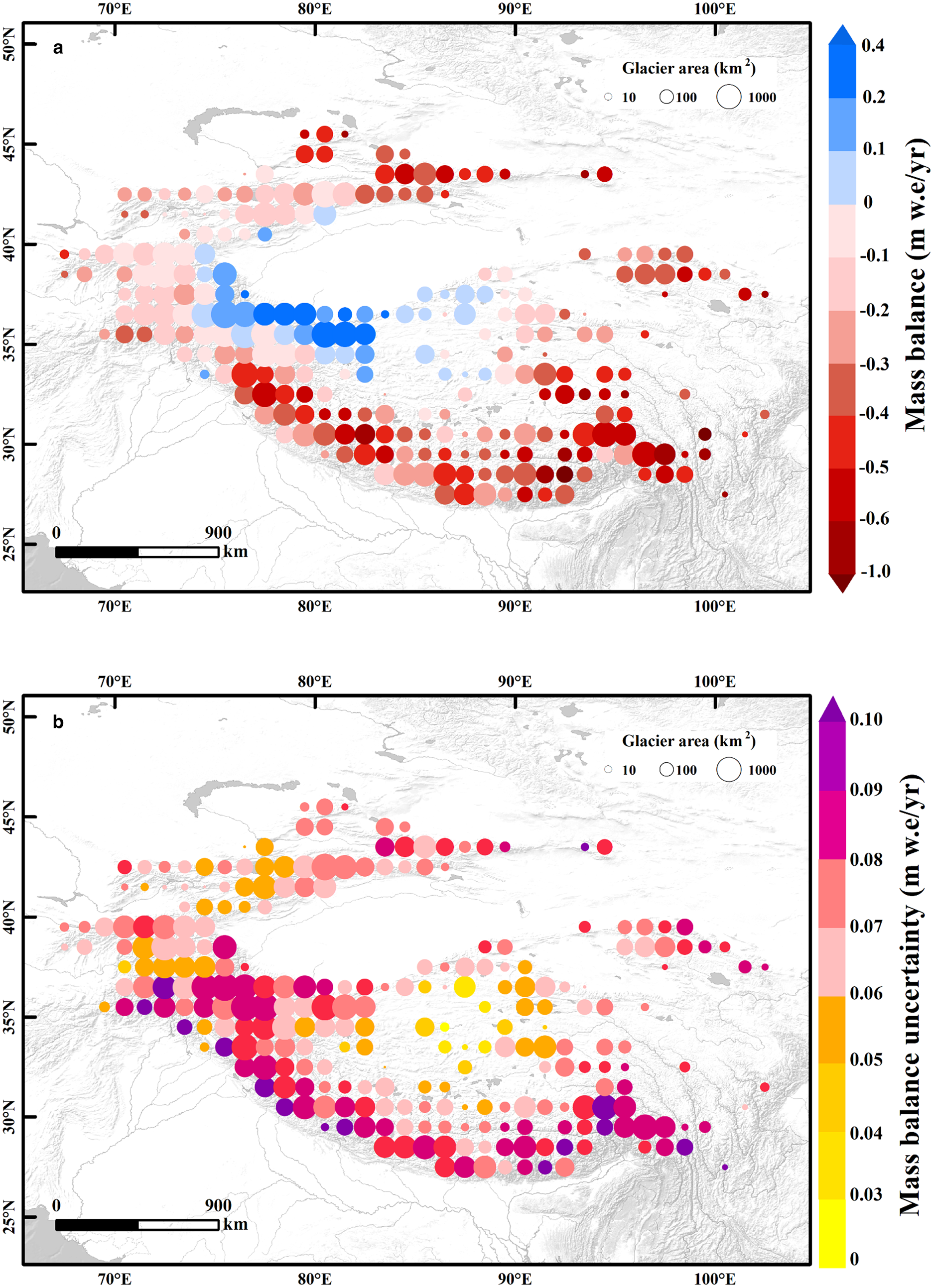
Fig. 4. Glacier mass-balance changes (a) and uncertainty (b) over the HMA for the period from 2000 to 2021. Data are shown on a 1° × 1° grid. The circle color represents the mass-balance variation, and the circle size is scaled according to the glacier area. Cells that do not match the glacier hypsometry were eliminated. Base map was from Esri, USGS, NOAA.
Mass changes varied among regions, with a decrease in glacier mass occurring in most sub-regions (Fig. 5). The Hengduan Shan experienced the highest rate of mass loss at −0.62 ± 0.10 m w.e. a−1 (−2.67 ± 0.45 Gt a−1), followed by the South and East Tibet Mountains with a mass change rate of −0.47 ± 0.11 m w.e. a−1 (−1.85 ± 0.43 Gt a−1). Moderate loss rates occurred in the central and northern HMA, and a negative mass rate ranging from −0.43 to −0.03 m w.e. a−1 was observed. Positive anomalies of 0.23 ± 0.13 m w.e. a−1 only occurred in the West Kun Lun Mountain.
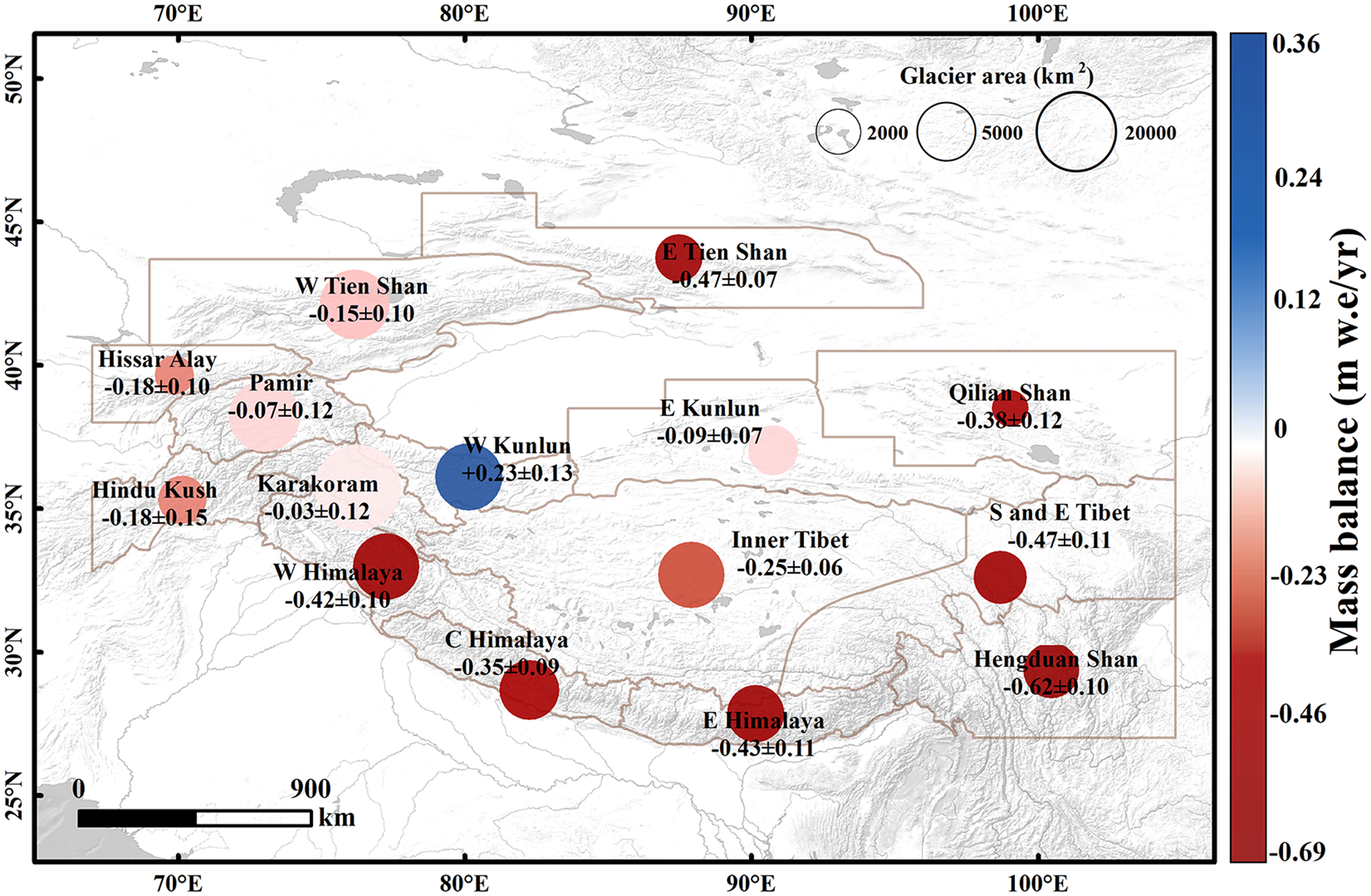
Fig. 5. Specific glacier mass balance (m w.e. a−1) for the period from 2000 to 2021, aggregated over the RGI mountain ranges. Sub-regions from HiMAP (Bolch and others, Reference Bolch, Wester, Mishra, Mukherji and Shrestha2019) and Kääb and others (Reference Kääb, Treichler, Nuth and Berthier2015) can be found in Figure S2.
3.3.2 Glacier mass budget of river basins
The spatial distribution of all river basins in HMA following the basin boundaries of Shean and others (Reference Shean2020) is shown in Figure 6. The most severe mass loss took place in the exorheic Brahmaputra, Ganges and Indus Basins and in the endorheic Ili and Amu Darya Basins. Only Tarim Basin showed a mass gain of +2.91 ± 1.82 Gt a−1.
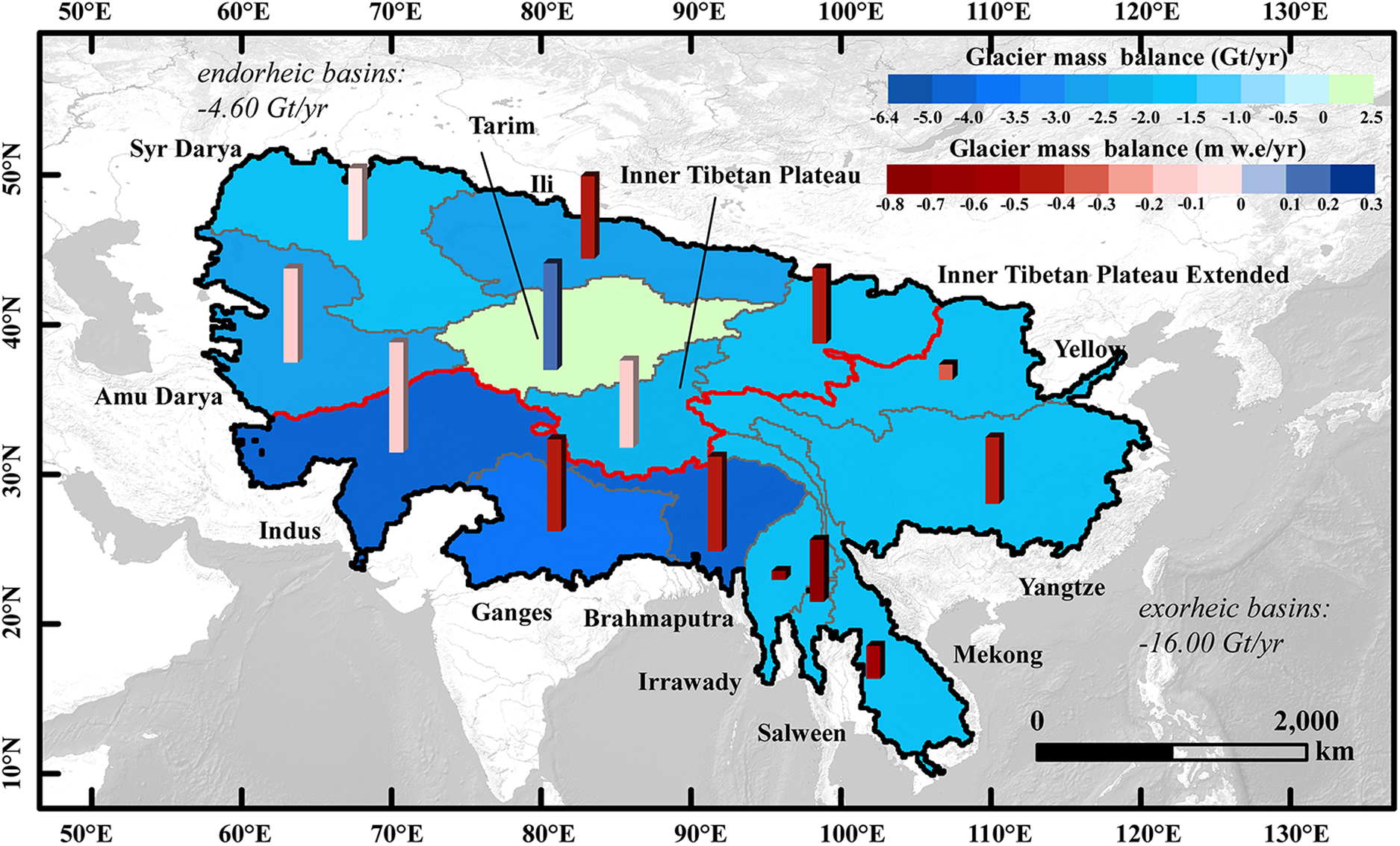
Fig. 6. Glacier excess melt runoff for the major river basins in HMA during 2000–2021. Colors of polygons denote the glacier runoff in Gt a−1, the heights of bars represent the sizes of the glacier in each basin, and the colors of bars represent the mass balance in units of m w.e. a−1. The red line indicates the dividing line of the exorheic and endorheic basins. Total mass losses were indicated in italics. Base map was from Esri, USGS, NOAA.
To estimate the contribution to sea level rise (SLR), we assume an ocean area of 3.62 × 10⁸ km2 (Jakob and others, Reference Jakob, Gourmelen, Ewart and Plummer2021). The excess discharge is 0 for glaciers with a balanced or positive mass budget (Brun and others, Reference Brun, Berthier, Wagnon, Kääb and Treichler2017), so we excluded Tarim Basin for further analysis. We considered two conditions for SLR contribution: from all basins and only from exorheic basins. The total potential contribution to SLR from all basins can be equivalated to a SLR of 0.055 ± 0.031 mm a−1. The total contribution from exorheic basins is equivalent to 0.043 ± 0.015 mm a−1.
4. Discussion
4.1 Penetration uncertainties/comparison
The offsets over debris-covered ice and off-glacier terrain are negative in few elevation bands of some sub-regions meaning that we observe a negative penetration. One main reason is the insufficiency of valid samples in the X-band SRTM data in these elevation zones. Another possible reason may be attributed to a biased correction in bedrock areas, due to inaccurate co-registration in high-relief regions (Li and others, Reference Li, Jiang, Liu and Wang2021). This kind of trend can also be seen in the penetration depths estimated by ICESat backpropagation (Kääb and others, Reference Kääb, Berthier, Nuth, Gardelle and Arnaud2012). In addition, the penetration depth is small at the high altitudes of Hissar Alay, Central Himalaya and East Himalaya Mountains, which may be connected to the spatial difference in the glacial distribution.
Secondly, the estimation of penetration depth varies with different estimation methods. Subtracting DEMs from field measurements or optical DEMs can provide accurate penetration depths, but is generally difficult to apply to the entire HMA region since there were no field or optical data available when the NASADEM data were acquired. Therefore, penetration depth can only be estimated through different assumptions. Methods proposed by Jaber and others (Reference Jaber, Rott, Floricioiu, Wuite and Miranda2019) and Zhou and others (Reference Zhou2019) rely on relative penetration depth differences between the X-band and C-band SRTM or NASADEM. We compare the relative penetration depth differences with previous studies (Table 2). The penetration depths we estimated agree well with those by Li and others (Reference Li, Jiang, Liu and Wang2021) except for the southern and south-eastern HMA. Li and others (Reference Li, Jiang, Liu and Wang2021) used the void-filled SRTM, which may contain fill-in pixels that are composed of different timestamps or from optical data. The void-filled portions are ~20% in the south-eastern HMA, thus the estimates derived from X-band SRTM and NASADEM are more consistent with those obtained by the non-void-filled SRTM (Zhou and others, Reference Zhou, Li, Li, Zhao and Ding2018, Reference Zhou2019). In addition, when we assumed that the average X-band penetration depth of 4 m and the percentage of dry snow area of 40% (i.e. the average SRTM X-band penetration of 1.6 m) (Zhou and others, Reference Zhou2019), the estimates by doubling the relative penetration differences generally agreed with them. However, it is difficult to quantify the percentage of dry snow area for each region in HMA, where each region has its own climatology.
Table 2. Estimated average NASADEM/C-band SRTM penetration depth (m) relative to the X-band SRTM
This study used non-void-filled NASADEM and X-band SRTM to estimate penetration differences. Li and others (Reference Li, Jiang, Liu and Wang2021) and Gardelle and others (Reference Gardelle, Berthier, Arnaud and Kääb2013) used X-band SRTM and the void-filled C-band SRTM, while Zhou and others (Reference Zhou, Li, Li, Zhao and Ding2018) masked out void-filled regions in the C-band SRTM to estimate penetration differences.
Furthermore, we compared the average penetration depth estimates of C-band radar proposed by Kääb and others (Reference Kääb, Berthier, Nuth, Gardelle and Arnaud2012). Compared with ICESat extrapolation, penetration estimates derived from doubling the relative penetration differences agreed well within the error bars in 10 of 15 regions (Table 1). Area with larger discrepancies located in the east HMA, especially the South and East Tibet Mountains and the Hengduan Shan mountains. ICESat only contained ~1000 on-glacier points in each measurement cycle in each sub-region, whereas the SRTM-X DEM can cover 10–40% glaciated areas. Hence, the difference mainly originated from the different sampled areas and elevations. The penetration depth of the C-band radar estimated by ICESat linear extrapolation was ~8–10 m in the south-eastern HMA (in both this study and that by Kääb and others (Reference Kääb, Berthier, Nuth, Gardelle and Arnaud2012)), which could have been overestimated, as this depth only occurs when the snow density is ~200 kg m−3 (Zhou and others, Reference Zhou, Li, Li, Zhao and Ding2018). On the contrary, the penetration depth estimates by ICESat extrapolation are smaller in East Kun Lun and Qilian Shan mountains. Estimates based on ICESat extrapolation may be suitable for areas with relatively consistent interannual elevation variations. Kääb and others (Reference Kääb, Berthier, Nuth, Gardelle and Arnaud2012) pointed out that the C-band penetration is also expected to be deeper on winter-accumulated glaciers than on summer-accumulated ones. The estimates derived from doubling the relative penetration differences are consistent with this assumption given the wider spatial coverage of X-band SRTM.
We finally considered the method of assuming that SRTM radar captured the 1999 autumn elevation profiles due to a reflective ice layer (Berthier and others, Reference Berthier, Arnaud, Vincent and Rémy2006) so that we could use ICESat-2 acquired during autumn season to calculate glacier mass balance. However, such a reflective-ice-layer assumption may work for lower glacier areas but may not be true for the upper accumulation areas in HMA where a distinct firn layer may not exist. C-band radar penetration is deeper in the accumulation areas in HMA, and the assumption may lead to much underestimated mass balance (Table S1).
For errors associated with radar penetration, we have considered the large uncertainties by using conservative error bars with the std dev. of the median penetration depths. Uncertainty in most regions exceeded 50% of the estimated region-mean penetration depths. As one of the significant sources of mass-balance uncertainty in using SAR-based DEMs, we provided a reference data for estimating regional glacier mass balance in HMA based on NASADEM, which may favor the increase of mass-balance accuracy.
4.2 Impact of NASADEM voids
The larger uncertainty in higher altitude regions is associated with the small number of laser footprints collected in glaciated areas. The larger uncertainty may also be attributed to the larger errors in the NASADEM on steeper slopes (Chen and others, Reference Chen2022) and the relatively larger percentage of voids compared to lower-slope regions.
The exclusion of void-filled areas in the NASADEM may introduce bias in the sampling (Kääb and others, Reference Kääb, Berthier, Nuth, Gardelle and Arnaud2012). We matched the glacier hypsometry of ICESat-2 and the void-filled NASADEM so that the area sampled by ICESat-2 is sufficiently representative of the entire region. Mass balance was calculated by comparing ICESat-2 and non-void-filled NASADEM because the void-filled portions may come from completely different data sources. The hypsometry difference between the void-filled and non-void-filled NASADEM may introduce additional uncertainty during mass-balance calculation. Therefore, we calculated the percentage of NASADEM voids in each sub-region. Different regions have different percentage of voids, and the regions that are most affected by voids are the Central Himalaya, followed by Hengduan Shan and South and East Tibet Mountains. Subsequently, we compared the hypsometry of the void-filled NASADEM and the non-void-filled NASADEM since the void-filled portions can serve as an elevation-range reference, and the two hypsometry results agreed well in 14 of 15 regions, except the South and East Tibet Mountain. Nonetheless, due to lack of measurements in the high altitudinal zones, it is difficult to apply the hypsometry filter; thus, we add an additional 10% of mass-balance uncertainty for the South and East Tibet Mountain in the final results. The voids are mostly distributed in the upper elevation zones, which are often above the mass equilibrium line, and any missing elevation measurements may cause the estimated mass balance toward a more negative value.
4.3 Comparisons with previous studies
Glacier mass balance in this study was generally consistent with other assessments. We found that the mass loss over the entire HMA during 2000–2021 is most similar to those derived from ASTER DEMs (Table 3). The sub-regional mass balances all showed the same spatial patterns with mass balance aggregated over the RGI regions (Table 4), Kääb boundary (Table S2) and HiMAP boundary (Bolch and others, Reference Bolch, Wester, Mishra, Mukherji and Shrestha2019) (Table S3). The glacier mass-balance estimates for the river basins in HMA also conformed to previous studies (Brun and others, Reference Brun, Berthier, Wagnon, Kääb and Treichler2017; Shean and others, Reference Shean2020) (Table S4), with the only difference occurring in the Tarim Basin. Results revealed a mass gain of +2.91 ± 1.82 Gt a−1 in Tarim from 2000 to 2021, while a mass loss of −0.87 ± 0.71 Gt a−1 was observed from 2000 to 2018 (Shean and others, Reference Shean2020).
Table 3. Previously published mass-balance estimates for HMA
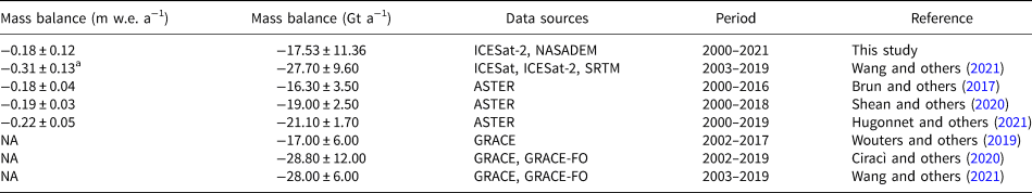
a Represents data obtained by elevation change by assuming the snow density of 850 ± 60 kg m−3, which is the same as the density assumption in other studies. NA indicates data not available in the reference.
Table 4. Region-wide mass balance compared with previous studies aggregated over the RGI boundary
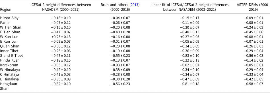
Linear-fit of ICESat/ICESat-2 height differences between NASADEM was obtained by following the method of Wang and others (Reference Wang, Yi and Sun2021). The result of ASTER DEMs during 2000–2019 was derived from the published elevation-change map by Hugonnet and others (Reference Hugonnet2021).
Mass-balance estimation by Hugonnet and others (Reference Hugonnet2021) is the recent research without the influence of radar penetration depth, the glacier mass balance derived from the elevation-change map can serve as a validation of absolute differencing of ICESat-2 and NASADEM. Wang and others (Reference Wang, Yi and Sun2021) used relative elevation differences between ICESat/ICESat-2 and void-filled SRTM, and performed a linear fit to the relative elevation differences to obtain glacier elevation change. Void-filled portions may bias the mass-balance estimates, so we recalculated the glacier mass balance using the non-void-filled NASADEM to make the comparison more robust. The glacier mass balances derived from absolute differencing of ICESat-2 and NASADEM tend to be less negative than those from the linear-fit (Table 4 and Fig. S3), although mostly within the error envelop, and we attributed the difference to the fewer ICESat footprints. The results show more consistency with the ASTER-based estimates (Table 4), but the elevation changes difference between the NASADEM and ASTER DEMs appear to be systematically biased. Taking the East Himalaya Mountain as an example, the glacier elevation changes in the low altitudes are more negative from the absolute differencing of ICESat-2 and NASADEM (Fig. S4), which might be associated with the penetration depth estimates tending to be slightly overestimated, but we have considered this penetration correction uncertainty in the accuracy assessment.
5. Conclusions
Radar penetration into snow/ice is essential for accurately estimating glacier mass balance based on the radar-derived NASADEM. To resolve the problem, we corrected the NASADEM DEM by doubling elevation differences between the SRTM X-band DEM and NASADEM. The glacier elevation and mass changes from 2000 to 2021 over the HMA region were then estimated by comparing the elevation differences of ICESat-2 and penetration depth corrected NASADEM.
We concluded that: (1) the penetration depths show an elevation-dependent pattern in which the penetration depth into the snow/ice by the C-band radar showed an upward trend with increasing elevation. Relatively larger average penetration depths occurred in the Himalaya and Hissar Alay mountain range, while smaller penetration depths were found in the South and East Tibet and Hengduan Mountains; (2) from 2000 to 2021, the glacier mass balance of HMA was −0.18 ± 0.12 m w.e. a−1 (−17.53 ± 11.36 Gt a−1), where the greatest mass loss occurred in the south-eastern HMA. Compared with previous studies, the West Kun Lun Mountain experienced a more conspicuous mass gain at a rate of 0.19 ± 0.13 m w.e. a−1; (3) the HMA glaciers have experienced mass losses in all basins but the Tarim basin, with the largest loss of −4.99 ± 2.05 Gt a−1 in the exorheic Indus basin, and the excessive glacier melt runoff of HMA was equivalent to a SLR of 0.055 ± 0.031 mm a−1.
The glacier mass balance during 2000–2021 yielded the same spatial patterns as previous studies, and the conformity of DEM-derived mass-balance estimates confirm the necessity of penetration depth correction for the NASADEM. ICESat-2 can be used to estimate glacier mass balance by comparing it with DEMs directly for regions where ICESat-2 data have a reasonable altitudinal distribution.
Supplementary material
The supplementary material for this article can be found at https://doi.org/10.1017/jog.2022.78.
Acknowledgements
We thank Etienne Berthier for his valuable suggestions, which significantly improved the quality of the manuscript. This work was supported by National Natural Science Foundation of China (grant No. 41830105 and 42011530120). The ICESat-2 data used in this study were obtained from the National Snow and Ice Data Center (http://nsidc.org). The NASADEM data were obtained from NASA (https://search.earthdata.nasa.gov/), and the SRTM X-band DEM were obtained from German Aerospace Center (https://download.geoservice.dlr.de/SRTM_XSAR/). The glacier boundaries were obtained from http://www.glims.org/RGI/rgi60_dl.html.


 Open access