


1. Introduction
Recent years have seen a surge of interest in deterministic wave forecasting for marine decision support systems, a sector that is poised to continue to grow along with further investment in the marine environment. Increasing the efficiency and safety of offshore renewable energy, autonomous shipping and navigation, and supply and offload operations from very large floating structures (see e.g. Zhao et al. Reference Zhao, Milne, Efthymiou, Wolgamot, Draper, Taylor and Eatock Taylor2018) relies on accurate, timely forecasts of wave conditions.
Such operations cannot rely on well-developed stochastic wave forecasts, which provide information of a space/time-averaged nature, on typical scales of  ${\sim }100\ \textrm {km}$ and
  ${\sim }6\ \textrm {h}$. Rather, a deterministic approach is needed, valid over typical scales of
  ${\sim }1\ \textrm {km}$ and
  ${\sim }5\ \textrm {min}$. The information provided about the sea state can then be used to calculate forces and moments on ships or structures (Kusters et al. Reference Kusters, Cockrell, Connell, Rudzinsky and Vinciullo2016), inform decisions about the feasibility of marine operations (Belmont et al. Reference Belmont, Christmas, Dannenberg, Hilmer, Duncan, Duncan and Ferrier2014), or provide input to adaptive control systems (Fusco & Ringwood Reference Fusco and Ringwood2010; Ma et al. Reference Ma, Sclavounos, Cross-Whiter and Arora2018).
Deterministic wave forecasting is a two-step process: (i) the sea-surface elevation (or some proxy thereof) must be measured, and (ii) the spatio-temporal evolution of that measurement must be computed. Both steps present unique theoretical and practical challenges, although herein only those associated with step (ii) will be addressed. Even if precise information about the sea state is available, the fact that waves in deep water are dispersive produces the major limitation to prediction. At lowest order, the phase velocity  $c_p$ of the waves is given by
  $c_p = \omega /k$ for
  $\omega ^2 = g|k|$ the deep-water dispersion relation, with
  $g$ the acceleration of gravity,
  $\omega$ the radian frequency and
  $k$ the wavenumber. Thus waves of different frequencies propagate at different speeds. Moreover, the energy of a wave group moves at the so-called group velocity
  $c_g = \textrm {d}\omega /\textrm {d}k$, and in deep water
  $c_g = c_p/2$. Therefore, waves within a measured area will move out of it at different speeds, and will mix with other waves originating outside that area. The theoretical region that is amenable to prediction is usually called the ‘predictable zone’. When the finite steepness of the waves is accounted for, it can be seen that amplitudes also have an influence on the frequencies, altering the dispersion relation, and thereby the predictable zone. All of these factors impact the ability to produce a forecast from measured data.
For usable forecasts, the sea state must be measured remotely, and for most applications the measurement technique of choice is based on marine wave radar (Borge et al. Reference Borge, Rodríquez Rodríguez, Hessner and González2004). Many existing applications (e.g. Connell et al. Reference Connell, Rudzinsky, Brundick, Milewski, Kusters and Farquharson2015; Hilmer & Thornhill Reference Hilmer and Thornhill2016; Al-Ani, Belmont & Christmas Reference Al-Ani, Belmont and Christmas2020) of deterministic forecasting, both research and commercial, make use of X-band radar backscatter (see Young, Rosenthal & Ziemer Reference Young, Rosenthal and Ziemer1985; Lee et al. Reference Lee, Barter, Beach, Hindman, Lake, Rungaldier, Shelton, Williams, Yee and Yuen1995; and others), although approaches based on LIDAR have also been advanced (see e.g. Belmont et al. Reference Belmont, Horwood, Thurley and Baker2007; Grilli, Guérin & Goldstein Reference Grilli, Guérin and Goldstein2011). X-band radar has the advantage of a large existing hardware base, as well as greater range, reflecting the relatively greater maturity of the technology.
No matter the source, wave measurements inevitably suffer from a number of uncertainties. Wave buoy measurements exhibit deviations from the actual sea state due to the buoy response (McAllister & van den Bremer Reference McAllister and van den Bremer2019), while radar is limited by wave shadowing (Plant & Farquharson Reference Plant and Farquharson2012) (the inability to observe in the radar shadow of a wave crest). While an accurate measurement of the sea-surface height at a single instant, like that furnished by the WASS (wave acquisition stereo system) of Fedele et al. (Reference Fedele, Benetazzo, Gallego, Shih, Yezzi, Barbariol and Ardhuin2013), would be ideal, radar measurements are further impacted by the rotation time of the radar antennae (typically several seconds (Al-Ani et al. Reference Al-Ani, Belmont and Christmas2020)). Moreover, the spacing of the measurement points cannot be determined a priori (Desmars et al. Reference Desmars, Bonnefoy, Grilli, Ducrozet, Perignon, Guérin and Ferrant2020). This issue was recently addressed by Qi et al. (Reference Qi, Wu, Liu and Yue2018b), who provided a very general formulation of the predictable region based on multiple spatio-temporal measurements, both fixed and moving.
For practical forecasts, with a time horizon limited to several minutes, it is imperative that the forecast is produced quickly. For this reason, linear wave propagation, with its low computational demands, has been widely used (Hilmer & Thornhill Reference Hilmer and Thornhill2016; Kusters et al. Reference Kusters, Cockrell, Connell, Rudzinsky and Vinciullo2016; Al-Ani et al. Reference Al-Ani, Belmont and Christmas2020). This means that such factors as wave–wave interaction, as well as the presence of bound modes, are necessarily missed. Since the importance of these, and the time scale of nonlinear evolution (theoretically  $\epsilon ^{-2}$ times a typical wave period in deep water, where
  $\epsilon$ is the wave steepness), depends on the wave steepness, linear theory may be appropriate for short-term predictions of quiescent states for some marine operations (Belmont et al. Reference Belmont, Christmas, Dannenberg, Hilmer, Duncan, Duncan and Ferrier2014). Nevertheless, considerable recent research has been devoted to nonlinear deterministic forecasting.
Early work on nonlinear wave forecasting used classical perturbation theory up to second order for unidirectional (Zhang et al. Reference Zhang, Chen, Ye and Randall1996) and short-crested waves (Zhang et al. Reference Zhang, Yang, Wen, Prislin and Hong1999). This relied on a division of the amplitude spectrum into frequency bands, with assumptions about distinct interactions between wave modes in each band. Subsequent work, starting with Wu (Reference Wu2004), sought to extend the order of nonlinearity and the physics accounted for by using the high-order spectral method (HOS) formulated by West et al. (Reference West, Brueckner, Janda, Milder and Milton1987) and Dommermuth & Yue (Reference Dommermuth and Yue1987). This method employs Zakharov's (Reference Zakharov1968) reformulation of the water-wave problem, together with eigenfunction expansion at each order, to account for arbitrary nonlinearity and large numbers of free modes (see e.g. Mei, Stiassnie & Yue Reference Mei, Stiassnie and Yue2018).
Since then, numerous studies have appeared on deterministic wave forecasting using HOS, including Köllisch et al. (Reference Köllisch, Behrendt, Klein and Hoffmann2018), who supplemented the HOS with a Newton–Krylov method for determining initial conditions, rather than the optimization procedures employed in Wu (Reference Wu2004) or Blondel, Bonnefoy & Ferrant (Reference Blondel, Bonnefoy and Ferrant2010). Qi et al. (Reference Qi, Wu, Liu, Kim and Yue2018a) employed HOS to extend the general linear predictable zone of Qi et al. (Reference Qi, Wu, Liu and Yue2018b), as well as comparing with tank data. They emphasize the importance of nonlinearity in reconstructing a sea state, and develop a method to optimize this reconstruction for a given number of wave modes. Klein et al. (Reference Klein, Dudek, Clauss, Hoffmann, Behrendt and Ehlers2019) subsequently investigated the use of HOS for a variety of different sea states, and used a surface similarity parameter to quantify the accuracy of the forecast. Law et al. (Reference Law, Santo, Lim and Chan2020) recently used an artificial neural network trained with HOS simulations to produce predictions. Desmars et al. (Reference Desmars, Bonnefoy, Grilli, Ducrozet, Perignon, Guérin and Ferrant2020) have developed a nonlinear Lagrangian model (see Guérin et al. Reference Guérin, Desmars, Grilli, Ducrozet, Perignon and Ferrant2019) and employed this for forecasting from non-uniformly spaced data from both HOS simulations and experiments.
Other approaches to nonlinear forecasting focus on using particular closed-form equations, such as the narrow-band cubic Schrödinger equation (NLS), and its extensions (Trulsen Reference Trulsen2005; Simanesew et al. Reference Simanesew, Trulsen, Krogstad and Nieto Borge2017). Such model equations have the advantages of providing analytical insight and tractability, as well as computational efficiency, albeit with some loss of predictability for broad-banded or short-crested seas. Klein et al. (Reference Klein, Dudek, Clauss, Ehlers, Behrendt, Hoffmann and Onorato2020) have compared several nonlinear Schrödinger models to HOS in a variety of conditions, and found that the inclusion of higher-order dispersion in NLS is crucial in achieving accuracy over a variety of conditions.
In the present paper we pursue wave forecasting using the Zakharov equation (Zakharov Reference Zakharov1968), a natural extension of the NLS that has not hitherto been used for this purpose. The Zakharov equation includes wave–wave interaction up to third order and yields the NLS and its extensions as narrow-band simplifications. It also serves as the basis for deriving Hasselmann's kinetic equation, which is widely used in (phase-averaged) oceanic wave forecasting models. Owing to a lack of bandwidth restriction and an explicit separation of resonant and non-resonant terms, the Zakharov formulation is simultaneously general and able to furnish detailed insight into the dominant nonlinear interactions for deep-water waves. Moreover, it is possible to distinguish among those nonlinear interactions which give rise to energy exchange, and those which effect only a mutual frequency correction among waves. Isolating this frequency correction yields a computationally simple but remarkably effective forecast. By revisiting the non-resonant contributions, it is likewise possible to isolate the contribution of bound modes to the evolution of a sea state.
In § 2 we describe how a reference ocean surface can be generated computationally to provide the basis for a forecast, and subsequently give a brief overview of some key concepts relating to discrete data points and Fourier transforms, which will be used for forecasting. In § 3 we introduce three possibilities for the time evolution of the forecast. These are linear frequency dispersion, weakly nonlinear amplitude dispersion derived from the Zakharov equation, or weakly nonlinear amplitude dispersion with energy exchange (using the Zakharov equation). The concept of a predictable region, and its dependence on linear and nonlinear forecasting, are discussed in § 3.2. Numerical results are provided in § 4: narrow spectra from the Joint North Sea Wave Observation Project (JONSWAP) are explored in § 4.1, and examples with broad Pierson–Moskowitz (PM) spectra are treated in § 4.2. Then § 4.3 looks at the inclusion of second-order bound modes and their effect on the forecast; and § 4.4 applies the forecasting methodology to reference seas generated by HOS. Finally § 5 provides some concluding remarks and directions for future research.
2. Synthetic sea surfaces and measurements
2.1. The synthetic sea surface
A computational study of the effects of nonlinearity on deterministic wave forecasting requires that realizations of various sea surfaces are available. Samples from these furnish the measurements that drive the forecast, and those forecasts are compared with subsequent spatio-temporal pictures of the sea surfaces. In common with much other work on deterministic forecasting (see e.g. Desmars et al. Reference Desmars, Perignon, Ducrozet, Guérin, Grilli and Ferrant2018; Klein et al. Reference Klein, Dudek, Clauss, Ehlers, Behrendt, Hoffmann and Onorato2020; Law et al. Reference Law, Santo, Lim and Chan2020), engineering design spectra will be used to generate the synthetic sea surfaces herein. These design spectra provide the basic parameters of the synthetic sea surface. For the time evolution of these sea surfaces, we will largely employ the Zakharov equation, which includes the effects of cubic nonlinearities. To incorporate higher-order nonlinearities, we also use the HOS method developed by Dommermuth & Yue (Reference Dommermuth and Yue1987) and West et al. (Reference West, Brueckner, Janda, Milder and Milton1987) to propagate our synthetic sea surfaces (see § 4.4).
The following steps towards generating and propagating the sea surface will be outlined in detail below: (i) select a continuous wavenumber spectrum; (ii) discretize the spectrum with a suitably dense number of modes  $M$; (iii) relate the
  $M$ modal amplitudes to complex amplitudes
  $B_i$ in the Zakharov formulation; (iv) use the
  $B_i$ to write the free surface
  $\eta = \eta _1 + \eta _2 + O(\epsilon ^3)$, including leading-order terms in
  $\eta _1$ and second-order bound modes in
  $\eta _2$; and (v) employ the Zakharov equation to calculate the temporal evolution of
  $\eta$ above.
The JONSWAP spectrum is widely used in engineering design, and gives a useful representation of energy density for a variety of wind conditions, including for stormy seas. The spectral shape is
 \begin{equation} \varPsi(k) = \frac{\alpha}{2 k^3} \exp\left(-\frac{5}{4} \left(\frac{k}{k_p}\right)^{{-}2} \right) \gamma^{\exp(-(\sqrt{{k}/{k_p}}-1)^2/(2 \sigma^2))}, \end{equation}
depending on wavenumber  $k$, with peak wavenumber
  $k_p$ and tunable parameters
  $\alpha$,
  $\gamma$ and
  $\sigma$. The PM spectrum, a common one-parameter representation of a fully developed sea, is obtained from (2.1) by setting the peak-sharpening parameter
  $\gamma =1$ and
  $\alpha =0.0081$. It is important to note that any spectrum is essentially a linear concept, drawing on the idea that a free surface can be described as a superposition of sinusoidal wave modes (see e.g. Holthuijsen Reference Holthuijsen2007).
To generate a synthetic sea surface, the wavenumber spectrum  $\varPsi (k)$ (either JONSWAP or PM) must first be discretized into a large number of wavenumber ‘bins’
  $k_i$, with
  $2\varPsi (k_i) \Delta k = a_i^2$ giving the corresponding mode amplitude, where
  $\Delta k$ is the width of each bin. This dense discretization furnishes the (initial) magnitude of the complex amplitudes
  $|B_k|$ via
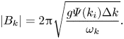 \begin{equation} |B_k| = 2{\rm \pi} \sqrt{\frac{g \varPsi(k_i) \Delta k}{\omega_k}}. \end{equation}
The phases  $\phi _k$ corresponding to the magnitudes
  $|B_k|$ are arbitrary, and play no role in the energy spectrum
  $\varPsi (k)$, which is predicated on an assumption of a spatially homogeneous and temporally stationary sea.
To third order in the wave steepness  $\epsilon$, the complex amplitudes evolve according to the Zakharov equation
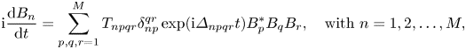 \begin{equation} \textrm{i} \frac{\textrm{d}B_n}{\textrm{d}t} = \sum_{p,q,r =1}^M T_{npqr} \delta_{np}^{qr} \exp({\textrm{i} \varDelta_{npqr} t}) B_p^* B_q B_r, \quad \text{with } n = 1, 2, \ldots , M, \end{equation}
where  $T_{npqr}=T({k}_n,{k}_p,{k}_q,{k}_r)$ are lengthy kernels (Mei et al. Reference Mei, Stiassnie and Yue2018),
  $\delta _{np}^{qr}$ is a Kronecker delta function such that
 \begin{equation} \delta_{np}^{qr} = \begin{cases} 1, & \text{for } {k}_n+{k}_p={k}_q+{k}_r,\\ 0, & \text{otherwise}, \end{cases} \end{equation}
and  $\varDelta _{npqr} = \omega _n + \omega _p - \omega _q - \omega _r$ is a frequency detuning. This equation captures energy exchange and nonlinear frequency correction due to resonant and near-resonant interactions of quartets of waves (see Mei et al. Reference Mei, Stiassnie and Yue2018). This is implicit in the derivation, and requires the frequency detuning to be small in an appropriate sense. (For computational implementation of the Zakharov equation, the criterion
  $\varDelta _{npqr}/\omega _p < \epsilon ^2$ is used, where
  $\omega _p$ is the peak frequency of the input spectrum, and
  $\epsilon$ an average steepness.) The Zakharov equation thus contains as special cases the third-order Stokes waves, the nonlinear wave–wave interactions of Longuet-Higgins & Phillips (Reference Longuet-Higgins and Phillips1962), the nonlinear Schrödinger equation (Zakharov Reference Zakharov1968) and many other phenomena.
The leading-order free-surface elevation  $\eta _1$ is obtained from the complex amplitudes via
 \begin{equation} \eta_1(x,t) = \frac{1}{2 {\rm \pi}} \sum_n \left( \frac{\omega_n}{2 g} \right)^{1/2} [ B_n\exp({\textrm{i}({k}_n {x} - \omega_n t)}) + \text{c.c.} ], \end{equation}
where ‘c.c.’ stands for the complex conjugate of the preceding expression. The next-order surface elevation  $\eta _2$ is associated with second-order bound harmonics. These arise due to non-resonant interactions, i.e. the linear harmonic wave description gives rise at second order to terms that include sums and differences of wavenumbers and frequencies like
 \begin{equation} \exp[\textrm{i}(k_i \pm k_j)x - (\omega(k_i) \pm \omega(k_j))t]. \end{equation}
Because  $\omega (k_i) \pm \omega (k_j) \neq \omega (k_i \pm k_j)$ in general, such bound modes do not propagate with the usual (linear or nonlinear) dispersion relation. For the same reason, these waves cannot fulfil both wavenumber and frequency resonance conditions. Their contribution to the free surface can be written in terms of complex amplitudes
  $B_i$ and kernels
  $V^{(1)}, V^{(2)}, V^{(3)}$ (see Mei et al. Reference Mei, Stiassnie and Yue2018, chap. 4.A) as
 \begin{align} \eta_2(x,t) &={-}\frac{1}{2 {\rm \pi}} \sum_{i,j=1}^{M/2-1} \sqrt{\frac{\omega_{i+j}}{2g}} \left( \frac{V^{(1)}_{i+j,i,j}}{\omega_{i+j} - \omega_i - \omega_j} + \frac{V^{(3)}_{{-}i-j,i,j}}{\omega_{i+j}+\omega_i+\omega_j} \right) \nonumber\\ &\quad \times \{ B_i B_j \exp[{\textrm{i}((k_i+k_j)x - (\omega_i+\omega_j)t)}] + \text{c.c.} \} \nonumber\\ & \quad + \, \sqrt{\frac{\omega_{j-i}}{2g}} \frac{V^{(2)}_{j-i,i,j}}{\omega_{j-i}+\omega_i-\omega_j} \{B_i^* B_j \exp[{\textrm{i}((k_j-k_i)x - (\omega_j - \omega_i)t)}] + \text{c.c} \}, \end{align}
where the shorthand notation 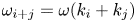 $\omega _{i+j}=\omega (k_i+k_j)$,
 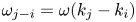 $\omega _{j-i}=\omega (k_j-k_i)$ and
  $V^{(n)}_{\pm i \pm j,\, i, j} = V^{(n)}(\pm k_i \pm k_j, k_i, k_j)$ is used.
Equations (2.5) and (2.7) together yield a free surface with sum and difference harmonics included, corresponding to the  $O(\epsilon )$ correction in Wehausen & Laitone (Reference Wehausen and Laitone1960, equation (27.25)). (For computational implementation, only modes that are in the support of the spectrum are considered, in order to prevent the accumulation of energy in high wavenumbers.) We will omit higher-order bound waves from the description of the free-surface, although these may be calculated from equation (14.3.5) of Mei et al. (Reference Mei, Stiassnie and Yue2018).
Thus, to obtain a realization of the reference ocean surface with particular statistical properties (such as significant wave height, or spectral peak period), initial magnitudes  $|B_n|$ are provided by (2.2) and initial phases
  $\phi _k$ are chosen randomly from a uniform distribution over
  $[0,2{\rm \pi} )$. Inserting these initial data into (2.5) yields a leading-order free surface, and inserting into (2.7) allows second-order bound modes to be added if desired. These reference ocean surfaces at
  $t=0$ will be measured (see § 2.2 below), and snapshots at
  $t>0$ (generated from numerical integration of (2.3)) will be compared to forecasts. The above formulation clearly separates the effects of nonlinearity on wave frequency and energy exchange (included in (2.5)) and the effects of nonlinearity on wave shape (included in (2.7)), allowing for the relative importance of bound modes to be examined.
2.2. Discrete measurements and the fast Fourier transform
Provided a free surface  $\eta (x,t)$ composed of long-crested unidirectional waves, we take samples at
  $N$ points
 \begin{equation} y_0, y_1, \ldots, y_{N-1}, \end{equation}
corresponding to a set of physical locations 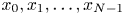 $x_0, x_1, \ldots , x_{N-1}$ at a specified time. It is simplest to assume that these data points are equally spaced, and so write
  $x_n = nL/N$, for
  $N$ samples covering a length
  $L-L/N$. Alternatively, for non-uniformly spaced points, a resampling based on interpolation can be used (see Desmars et al. (Reference Desmars, Bonnefoy, Grilli, Ducrozet, Perignon, Guérin and Ferrant2020) for an example of how non-uniformly sampled points may be treated). Then the discrete-time Fourier transform (DTFT) of the sequence
  $\{y_n\}_{n=0}^{N-1}$ is defined as
 \begin{equation} Y(\,j) = \sum_{n=0}^{N-1} y_n \exp(-\textrm{i} 2 {\rm \pi}j n /N) = \sum_{n=0}^{N-1} y_n \exp(-\textrm{i} k_j x_n), \end{equation}
for  $k_j = 2 {\rm \pi}j/L$.
Since  $Y(\,j+N) = \sum _n y_n \exp (-\textrm {i} 2{\rm \pi} j n/N) \exp (-\textrm {i}2{\rm \pi} n) = Y(\,j)$, the new sequence is
  $N$-periodic. The
  $Y(\,j)$ are the discrete-time Fourier coefficients, obtained by multiplying the original sequence by the
  $N$th complex roots of unity, and may be efficiently calculated using the fast Fourier transform (FFT).
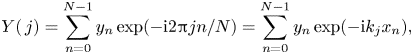
The inverse transform is given by
 \begin{equation} y_n = \frac{1}{N} \sum_{m=0}^{N-1} Y(m) \exp(\textrm{i} 2 {\rm \pi}m n /N), \end{equation}
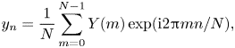
which yields an  $N$-periodic extension of the original sequence. Moreover, it is possible to construct a continuous signal by replacing
  $nL/N$ by a continuous variable
  $x$:
$x$:
 \begin{equation} y(x) = \frac{1}{N} \sum_{m=0}^{N-1} Y(m) \exp(\textrm{i} k_m x). \end{equation}
For  $N$ even, it will be convenient for subsequent computations to rewrite (2.11) in the form
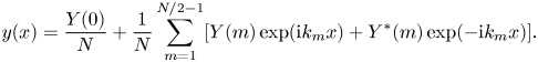 \begin{equation} y(x) = \frac{Y(0)}{N}+\frac{1}{N} \sum_{m=1}^{N/2-1} [ Y(m) \exp(\textrm{i} k_m x) + Y^*(m) \exp(-\textrm{i} k_m x) ]. \end{equation}
The first term  $Y(0)/N$ is the mean of the sampled points by (2.9) – an approximation to the mean sea surface over the measurement area. The forecast is thus prepared using
  $N/2-1$ distinct Fourier modes, which should be significantly smaller than, and not a subset of, the
  $M$ modes in the generated sea.
3. Deterministic forecasting
3.1. Linear and nonlinear forecasts
Section 2.2 describes the process of  $(a)$ taking a continuous sea-surface elevation,
  $(b)$ measuring it at
  $N$ equidistant points
  $x_n = nL/N$,
  $(c)$ computing the FFT of the measured sequence, and
  $(d)$ using the inverse transform to construct an
  $L$-periodic, continuous approximation to the original sea. That approximation will form the basis for a leading-order forecast, with different possibilities for its forward evolution in time. The possibilities to be explored here are: (i) linear dispersion, assuming modes
  $k_n$ have a frequency
  $\omega _n = \sqrt {g |k_n|}$; (ii) Stokes’ corrected dispersion, where the linear frequency is corrected by the presence of other waves to
  $\varOmega _n = \omega _n + \sum _p e_{np} T_{npnp} |B_p|^2$; and (iii) third-order nonlinear evolution using the Zakharov equation.
The simplest spatio-temporal forecast is obtained by assuming that propagating modes are governed by the linear dispersion relation  $\omega _m = \sqrt {g |k_m|}$, which establishes a one-to-one correspondence between wavenumbers
  $k \in \mathbb {R}^+$ and (positive) frequency. For unidirectional propagation, this allows for a linear forecast
  $\zeta _L$ to be constructed directly from the Fourier coefficients via (2.12) to yield
 \begin{equation} \zeta_L(x,t) = \frac{Y(0)}{N} + \frac{1}{N} \sum_{m=1}^{N/2-1} [ Y(m) \exp(\textrm{i}( k_m x-\omega_m t)) + Y^*(m) \exp(-\textrm{i} ( k_m x - \omega_m t) ) ], \end{equation}
where the subscript ‘ $L$’ is used to denote linear dispersion.
Linear theory is predicated on assumptions of small wave steepness  $\epsilon$. Thus, for steeper waves, a number of nonlinear effects manifest:
(i) amplitude-dependent, mutual frequency correction of different wave modes; and
(ii) slow energy exchange among resonant and near-resonant wave modes.
The simplest way to exploit the Zakharov formulation is to employ it to calculate an analogue of Stokes’ frequency correction, whereby the finite amplitude affects the dispersion relation of waves. This was first demonstrated for a single wave mode by Stokes (Reference Stokes1847), for two wave modes by Longuet-Higgins & Phillips (Reference Longuet-Higgins and Phillips1962), extended to include the effects of surface tension by Hogan, Gruman & Stiassnie (Reference Hogan, Gruman and Stiassnie1988), and subsequently to many modes (Stiassnie Reference Stiassnie1991) and finite depth (Madsen & Fuhrman Reference Madsen and Fuhrman2012).
The Zakharov equation (2.3) makes the calculation of the mutual frequency correction algebraically simple: assuming that the magnitude of the complex amplitudes is constant, so  $|B_n(t)| = |B_n(0)|$, the Zakharov equation can be integrated in time to leading order, as described by Stuhlmeier & Stiassnie (Reference Stuhlmeier and Stiassnie2019). This leads to the compact expression for the nonlinear frequency correction
 \begin{equation} \varOmega_n = \omega_n + \sum_p e_{np} T_{npnp} |B_p|^2, \end{equation}
where  $\omega _n$ is the linear frequency,
  $\varOmega _n$ the nonlinear corrected frequency and
 \begin{equation} e_{np} = \begin{cases} 1, & \text{for } n = p,\\ 2, & \text{for } n \neq p. \end{cases} \end{equation}
For long-crested waves, as those treated herein, the kernel  $T_{npnp}$ takes the following simple form:
 \begin{equation} T(k_n,k_p,k_n,k_p) = \begin{cases} \dfrac{k_n k_p^2}{4 {\rm \pi}^2}, & \text{for } 0< k_p < k_n , \\ \dfrac{k_n^2 k_p}{4 {\rm \pi}^2}, & \text{for } k_p \geq k_n >0. \end{cases} \end{equation}
Comparing (2.12) and (2.5), the rescaling between Fourier amplitudes  $Y(m)$ and initial values for the complex amplitudes
  $B_m$ is
 \begin{equation} B_m(0) = \frac{2 {\rm \pi}}{N} \sqrt{\frac{2 g}{\omega_m}} \, Y(m), \end{equation}
for  $N$ the number of sampling points, and
  $m=1,\ldots ,N/2-1$, so that the measured sea-surface elevation provides all the ingredients for calculating the corrected frequencies.
In turn, this allows for a second forecast, improving upon (3.1):
 \begin{align} \zeta_S(x,t) = \frac{Y(0)}{N} + \frac{1}{N} \sum_{m=1}^{N/2-1} [ Y(m) \exp(\textrm{i}( k_m x-\varOmega_m t)) + Y^*(m)\exp(-\textrm{i} ( k_m x - \varOmega_m t) ) ]. \end{align}
Here the subscript ‘ $S$’ is used to denote Stokes’ corrected dispersion. The measured mode amplitudes
  $Y(m)$ remain constant, but the frequency
  $\varOmega _m$, as well as phase and group velocities, depend on those amplitudes through (3.2).
Finally, it is possible to include third-order energy exchange between quartets of waves in the forecast, allowing the mode amplitudes to be functions of time. The forecast is then cosmetically similar to (3.1):
 \begin{align} \zeta_Z(x,t) = \frac{Y(0)}{N} + \frac{1}{N} \sum_{m=1}^{N/2-1} [ Y(m,t) \exp(\textrm{i}( k_m x-\omega_m t)) + Y^*(m,t) \exp(-\textrm{i} ( k_m x - \omega_m t) ) ], \end{align}
The subscript ‘ $Z$’ is used to denote evolution using the Zakharov equation, and the argument of the (complex) terms
  $Y(m,t)$ contributes the nonlinear frequency correction seen in (3.6). This forecast entails numerical integration of
 \begin{align} \textrm{i} \frac{Y(m,t)}{\textrm{d}t} =\frac{8 {\rm \pi}^2 g}{N^2} \sum_{p,q,r=1}^{N/2-1} \left(\frac{\omega_m}{\omega_p \omega_q \omega_r} \right)^{1/2} T_{mpqr} \delta_{mp}^{qr} \exp({\textrm{i}\varDelta_{mpqr}t}) Y^*(p,t) Y(q,t) Y(r,t), \end{align}
where  $Y(i,0)$ are the Fourier coefficients obtained from the measurement. This is equivalent to solving a Zakharov equation with
  $N/2-1$ modes (with
  $N/2-1 < M$ for
  $M$ the number of modes in the sea). Here the initial amplitudes and phases are obtained from the measurements directly, whereas the initial data for the sea are initialized from a given spectrum. The
  $N$ surface-elevation measurements give only
  $N/2-1$ coupled Zakharov equations because the complex amplitudes
  $B_i$ depend on both the free surface and the potential at the free surface (see (2.12a,b) in Stiassnie & Shemer Reference Stiassnie and Shemer1984).
3.2. The predictable region
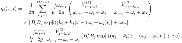
Owing to their dispersive nature, waves measured over a given area of ocean surface will travel through – and ultimately out of – that area at different speeds. Thus the group velocities of the longest and shortest waves in the measurement, denoted  $c_{g,L}$ and
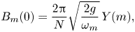
  $c_{g,S}$, respectively, determine the predictable region. Any deterministic forecast is thus time-limited, with the extent of the predictable region determined largely by the region of sea measured, and the group velocities of the waves therein. Because nonlinear effects change the dispersion relation, as encapsulated in (3.2), they also affect the group velocity, as depicted in figure 1. Since the effect of nonlinearity in (3.2) is to increase phase and group velocities versus linear theory (an effect also observed experimentally by Taklo et al. (Reference Taklo, Trulsen, Gramstad, Krogstad and Jensen2015)), in a manner dependent on the amplitudes of other waves in the sea, the extent to which the predictable region varies depends on
  $\epsilon$.
Figure 1. Predictable regions according to the linear (dashed lines) and nonlinear (solid lines) dispersion relations. The waves are derived from a JONSWAP spectrum with either  $\epsilon =0.1$ (a) or
  $\epsilon =0.2$ (b); see table 1. In panels (a) and (b),
  $c_{g,L}$ and
  $c_{g,S}$ are calculated for
  $k_L = 0.028\ \text {m}^{-1}$ and
  $k_S = 0.25\ \text {m}^{-1}$, respectively.
In figure 1 the predictable regions are shown using linear dispersion ( $\triangle ABC$) and nonlinear dispersion (
 $\triangle ABD$), with the lines
  $\overline {AC}$,
  $\overline {AD}$ and
  $\overline {BC}$,
  $\overline {BD}$ calculated for
  $k_L$ and
  $k_S$, respectively. For low (mean) steepness, the predictable regions are nearly identical, but, as steepness increases, the nonlinear theory allows for a theoretically larger, and slightly shifted, predictable region. (The predictable region increases in size because the nonlinear frequency correction disproportionately affects shorter waves; see the discussion in Stuhlmeier & Stiassnie (Reference Stuhlmeier and Stiassnie2019).) In what follows, we shall compare the forecast and the synthetic ‘sea’ within the nonlinear predictable region only.
4. Results
The above sections describe a procedure generating a synthetic sea from a spectrum, sampling that sea at a number of spatial locations, and using those measurements to generate a spatio-temporal forecast. Deriving the measurements from reference ocean surfaces generated from JONSWAP and PM wavenumber spectra as described in § 2.1 allows for the effects of nonlinearity on the forecast to be examined in detail. Moreover, many statistically identical realizations of the ocean surface can be generated to test each forecasting approach. A schematic of our forecasting approach using a JONSWAP spectral shape is given in figure 2.
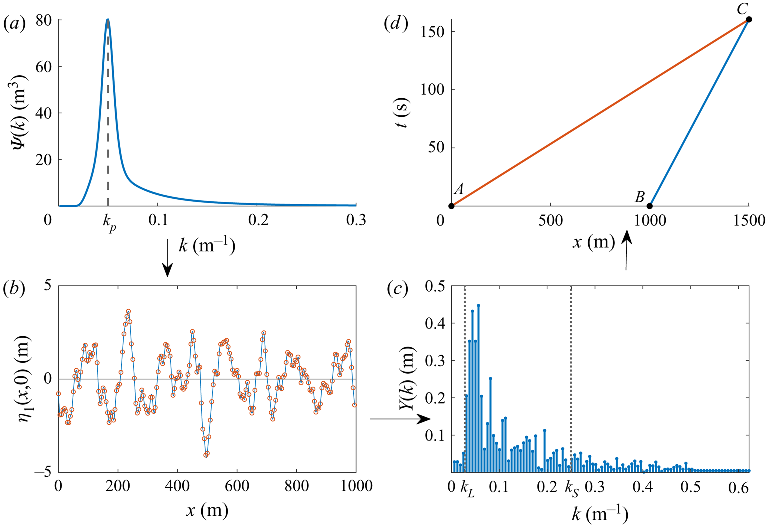
Figure 2. Schematic diagram for wave forecasting with a synthetic sea surface. Anticlockwise from top left: (a) JONSWAP energy spectrum with  $k_p=0.05\ \text {m}^{-1}$ and
  $\epsilon =0.1$. (b) A synthetic sea surface derived from the JONSWAP spectrum, here sampled at
  $N=200$ points (red circles) over
  $L=1000\ \textrm {m}$. (c) The FFT of the sampled values yields
  $N=200$ Fourier amplitudes. Only modes between
  $k_L=0.028\ \text {m}^{-1}$ and
  $k_S=0.25\ \text {m}^{-1}$ are retained as significant. (d) The group velocities
  $c_{g,L}$ and
  $c_{g,S}$ associated with
  $k_L$ and
  $k_S$ determine the predictable region
  $\triangle ABC$ of space–time. All the wave energy in modes
  $k \in [k_L, k_S]$ within the triangular region enters it through the segment
  $\overline {AB}$ at time
  $t=0$.
Figure 2(a) shows the JONSWAP energy spectrum  $\varPsi (k)$. This is used to generate a reference surface or ‘sea’
  $\eta _1(x,0)$, and in figure 2(b) the samples of the reference ocean surface are represented by red circles. As mentioned in § 3.1, it is convenient to choose these measurement points with uniform spacing in the
  $x$-direction. In real-world applications, the sampling length and measurement spacing might be constrained by the range and resolution of a shipboard X-band radar, but for our synthetic seas no such restrictions exist. Measuring at
  $N$ points over a length
  $L$ means that wave modes
  $k \in \{ 2 {\rm \pi}/L, 4 {\rm \pi}/L, \ldots , 2{\rm \pi} (N/2-1)/L\}$ can be resolved. Therefore,
  $L$ must be sufficiently large to resolve the longest waves of interest, and
  $N$ must be sufficiently large to avoid aliasing errors. The primary effect of selecting
  $L$ is to determine the size of the
  $x$–
$x$– $t$ domain for which prediction is possible.
Depending on the situation of interest, not all of the sampled modes may be relevant – particularly long or short waves may not have a significant effect on shipping, for example. To this end, a reduced set of modes  $k \in [ k_L, k_S]$ is used, which are depicted by the dotted vertical lines in figure 2(c). These represent the longest and shortest waves accounted for in the forecast.
Following § 3.2, the nonlinear predictable region  $\triangle ABC$, depicted in figure 2(d), is calculated. For waves travelling in the positive
  $x$-direction, measured waves
  $k \in [ k_L, k_S]$ will propagate through the region bounded by lines
  $\overline {AC}$ with slope
  $1/c_{g,L}$ and
  $\overline {BC}$ with slope
  $1/c_{g,S}$. As time progresses, waves shorter than
  $k_S$ (originating at
  $t=0$ at points
  $x>B$) will infiltrate the region
  $\triangle ABC$ from the right of
  $\overline {BC}$, and waves longer than
  $k_L$ (originating at points
  $x<A$) will do likewise from the left of
  $\overline {AC}$. In the scenario depicted, at
  $t=160\ \textrm {s}$ the information in the measurement region
  $\overline {AB}$ has completely dispersed, and no prediction can be made. In the examples below, we present the three forecasting techniques of § 3.1 applied to a variety of cases.
4.1. Examples based on JONSWAP spectra
In discretizing the spectrum we employ  $M=198$ wavenumber bins from
  $k=0.0012\ \text {m}^{-1}$ to
  $k=0.24\ \text {m}^{-1}$, with uniform spacing
  $\Delta k = 0.0012\ \text {m}^{-1}$. This gives the reference sea
  $\eta _1$ (without bound waves, calculated using (2.5) as described in § 2.1, and simulated in time with the Zakharov equation (2.3)) a spatial periodicity of
  $5236$ m. For simplicity, in figures and tables we denote the reference sea throughout by ‘Sea’. As shown in figure 2, we shall measure a stretch of this reference sea
  $L=1000\ \textrm {m}$ in length at
  $N=200$ measurement points to avoid errors in the short wavelengths. (The forecast is thus constructed from 99 Fourier modes, versus 198 modes in the synthetically generated sea. The former are not a subset of the latter.) As cutoff wavenumbers for the measured waves we take
  $k_L = 0.028\ \text {m}^{-1}$ and
  $k_S = 0.25\ \text {m}^{-1}$, so that the longest and shortest waves in the forecast are 224 and 25 m long, respectively (the peak of our JONSWAP spectrum corresponds to 126 m waves).
The parameter  $\alpha$ can be interpreted as an energy scale, and is proportional to the significant wave height and average slope as seen in table 1 (
 $\sigma = 0.08,\ \gamma = 5$ and peak wavenumber
  $k_p = 0.05\ \text {m}^{-1}$ are held constant).
Table 1. The JONSWAP parameter  $\alpha$ and corresponding
  $\epsilon$ and spectral significant wave height
  $H_{m_0}$. Other JONSWAP parameters are fixed at
  $\sigma = 0.08,\ \gamma = 5$ and
  $k_p = 0.05\ \text {m}^{-1}$.
In table 1 we use the integral of the spectrum
 \begin{equation} m_0 = \int \varPsi(k)\,\textrm{d}k \end{equation}
to define  $\epsilon =\sqrt {2 m_0}k_p$ and
  $H_{m_0}=4\sqrt {m_0}$.
Just as the predictable region depends on the nonlinearity of the sea state, so does the accuracy of the forecast itself. In figure 3 a number of forecasts are depicted compared to a reference sea initialized using a JONSWAP spectrum (as described above). Three mean steepness values  $\epsilon =0.1,\ 0.15$ and
  $0.2$ are shown (see table 1), and the sea at
  $t=60\ \textrm {s}$ is compared to forecasts using linear dispersion (3.1) and the Zakharov equation (3.7) (figure 3a,c,e), or linear dispersion (3.1) and nonlinear dispersion (3.6) (figure 3b,d,f). The theoretical predictable region at this time is bounded on the
  $x$-axis by two dashed vertical lines, which are determined from the group velocities of the longest and shortest waves accounted for.
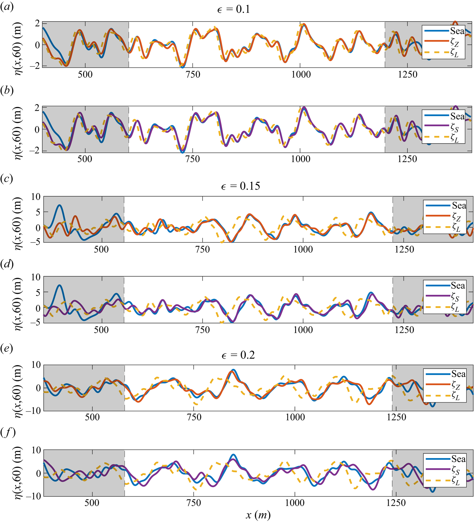
Figure 3. Comparison of forecasts with a reference sea  $\eta _1$ (blue solid line, denoted ‘Sea’) at
  $t=60\ \textrm {s}$, for
  $\epsilon = 0.1,\ 0.15$ and
  $0.2$. (a,c,e) The sea is compared to a linear forecast (yellow dashed line) and a forecast based on the Zakharov equation (red solid line). (b,d,f) The sea is compared to a linear forecast (yellow dashed line, as in a,c,e) and a linear forecast with nonlinear frequency correction (purple solid line).
For  $\epsilon =0.1$, all three forecasts agree reasonably well – there is little difference between linear and nonlinear dispersion, and scant energy exchange within the framework of the Zakharov equation. For
  $\epsilon =0.15$ the lower phase and group speeds of the linear theory lead to departures from the reference sea. Finally, for
  $\epsilon =0.2$, the evolving amplitudes become important, with the best agreement seen for the forecast based on the Zakharov equation. Nevertheless, the simpler forecast
  $\zeta _S$ continues to display satisfactory agreement.
It is possible to obtain a measure of the quality of the forecast in space and time by considering the difference between reference sea and forecast as in figure 4, which compares the sea and forecasts based on (3.6) and (3.7) throughout the predictable region. While both forecasts initially match the sea (at time  $t=0$, on the
  $x$-axis of both plots), the forecast based on integrating the Zakharov equation remains very accurate until at least
  $t=60\ \textrm {s}$, while the forecast based on nonlinear dispersion alone shows significant deviations, comparable to the significant wave height of the sea itself.
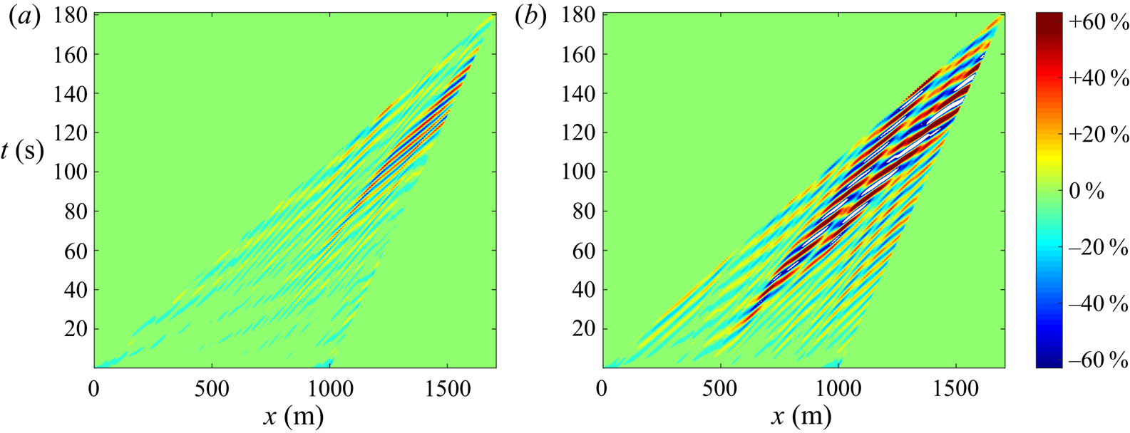
Figure 4. Signed difference between the reference ocean surface and (a) the forecast  $\zeta _Z$ computed from the Zakharov equation (3.7) or (b) the forecast
  $\zeta _S$ with nonlinear frequency correction (3.6). Only differences within the predictable regions (see figure 1) are shown, for a reference sea with
  $\epsilon = 0.15$ (see table 1). Colours denote the percentage of the significant wave height
  $H_{m_0}=8.5\ \textrm {m}$, and the area outside the predictable region is set to zero.
The comparisons shown in figures 3 and 4 are each based on a single realization of the reference ocean surface from a JONSWAP spectrum, so that the quality of the forecast will vary depending on those waves measured over the length  $L$ at
  $t=0\ \textrm {s}$. An aggregate measure of quality is provided by computing the linear correlation between forecast and sea, a simple measure of whether the forecast rises and falls with the reference sea. For two samples
  $x=\{x_1,\ldots ,x_n\}$ and
  $y=\{y_1,\ldots ,y_n\}$, Pearson's correlation coefficient is written as
 \begin{equation} \rho_{x,y} = \frac{\sum_{i=1}^n (x_i - \bar{x})(y_i-\bar{x})}{\sqrt{\sum_{i=1}^n (x_i-\bar{x})^2}\sqrt{\sum_{i=1}^n (y_i - \bar{y})^2}}, \end{equation}
where  $\bar {x}$ denotes the mean. The correlation coefficient ranges between
  $-1$ and
  $+1$, with 0 implying no linear correlation. A value of
  $+1$ means perfect positive correlation, e.g. crests in one signal coincide with crests in the second, while
  $-1$ means perfect negative correlation, where crests in one signal coincide with troughs in the second. Other aggregate measures of fit exist, including the ‘surface similarity parameter’ developed by Perlin & Bustamante (Reference Perlin and Bustamante2016) and used to investigate deterministic wave predictions in Klein et al. (Reference Klein, Dudek, Clauss, Ehlers, Behrendt, Hoffmann and Onorato2020).
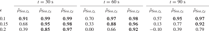
For the three values of  $\epsilon$ in table 1, the correlation
  $\rho$ between sea and forecast is computed at three forecasting times
  $t=30,\ 60$ and
  $90\ \textrm {s}$ throughout the predictable interval bounded by the nonlinear group velocities (see figure 1). Repeating this procedure with 50 realizations of the sea surface, each initialized with random, uniformly distributed phases, and averaging the correlation, yields the results shown in table 2, where
  $\bar {\rho }$ denotes the average correlation. Note that figure 3 is one representative realization for the middle column
  $(t=60\ \textrm {s}$) of table 2. To identify high-quality forecasts, those entries with mean correlation equal to or greater than 0.8 have been marked in bold. For short time and low mean steepness, all three forecasting methods are comparable. Even through intermediate time
  $t=60\ \textrm {s}$ and steepness
  $\epsilon =0.15$, the frequency-corrected forecast
  $\zeta _S$ in (3.6) performs very well. For severe seas associated with
  $\epsilon =0.2$, however, a forecast based on the Zakharov equation (3.7) is clearly preferable.
Table 2. Mean correlation between sea and forecast for  $t=30,\ 60$ and
  $90\ \textrm {s}$, with
  $\epsilon =0.1,\ 0.15$ and
  $0.2$. In each instance, 50 realizations of the reference ocean surface and corresponding forecasts are employed, and the mean correlation over the predictable interval is calculated. Mean correlations
  $\geq 0.8$ have been marked bold.
4.2. Forecasting for a broad spectrum
Because a forecasting approach based on the Zakharov equation has no bandwidth limitation, it is instructive to consider an example of forecasting for a fully developed sea provided by a PM spectrum, which is discretized using 200 wavenumber bins between 0.001 and 0.2. To compare with the results for a narrower spectrum in § 4.1, we select a PM spectrum with significant wave height 5.7 m (see table 1), which yields  $k_p=0.029$ and
  $\epsilon =0.056$ from (4.1). Since the PM spectrum represents a scenario of wind blowing over unlimited fetch, only one free parameter is available to describe such a fully developed sea.
Given the smaller peak wavenumber, the forecasting region must be increased in size in order to sample waves of interest. Consequently  $L$ is extended to 2000 m, and
  $N$ to 300 (hence 149 Fourier modes) to avoid aliasing errors (from
  $L=1000\ \textrm {m}$ and
  $N=200$ for the narrow spectra in § 4.1). In addition, the smallest and largest wavenumbers of interest for the forecast are chosen as
  $k_L = 0.01\ \text {m}^{-1}$ and
 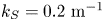 $k_S = 0.2\ \text {m}^{-1}$, so that the longest and shortest waves resolved are 628 m and 31 m in length, respectively. The increase in the measurement region leads to a concurrent increase in the predictable region.
A comparison of the three forecasts developed in § 3.1 for such a PM spectrum is given in figure 5. Owing to the low steepness of the sea ( $\eta _1$ calculated from (2.5), without bound waves), the linear forecast
  $\zeta _L$ proves excellent at
  $t=60\ \textrm {s}$ – the mean correlation over the predictable region from 50 realizations is 0.92 for the linear forecast, compared to 0.99 for
  $\zeta _S$ and 1.00 for
  $\zeta _Z$. For longer times, corrections to the dispersion relation (3.6) become increasingly important – the mean correlation from forecasting 50 realizations of the sea to time
  $t=120\ \textrm {s}$ decreases to 0.75 for
  $\zeta _L$, but remains 0.98 for
  $\zeta _S$ and 0.99 for
  $\zeta _Z$. For fully developed seas of such low steepness (
 $\epsilon =0.056$), the frequency-corrected forecast is nearly identical to the forecast based on the Zakharov equation (3.7).
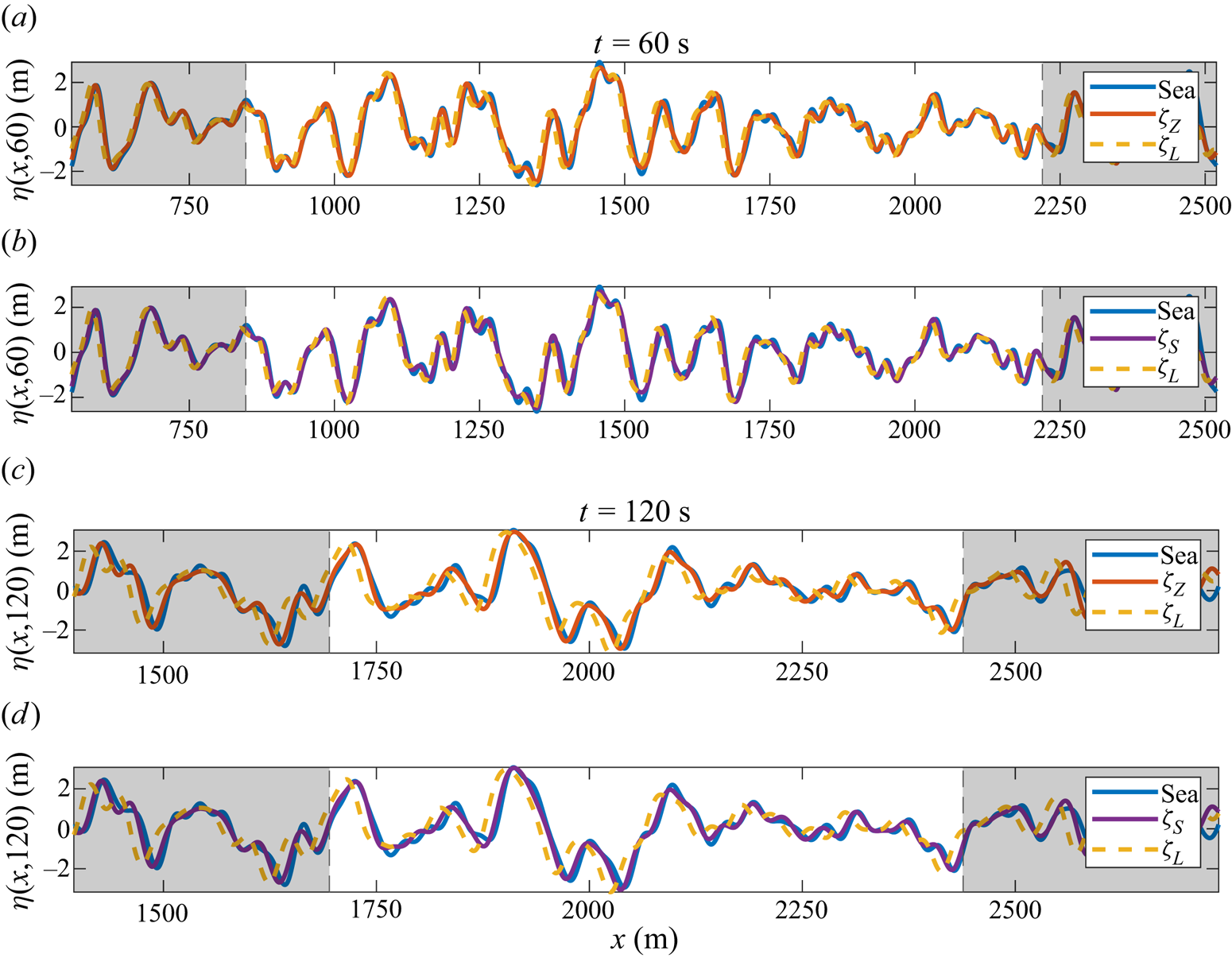
Figure 5. Comparison of forecasts with a reference sea  $\eta _1$ (blue solid line, denoted ‘Sea’) generated by a PM spectrum with
  $k_p = 0.029$ at
  $t=60\ \textrm {s}$ (a,b) and
  $t=120\ \textrm {s}$ (c,d). Dashed vertical lines represent the boundaries of the predictable region determined from the nonlinear group velocities of
 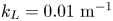 $k_L = 0.01\ \text {m}^{-1}$ and
  $k_S = 0.2\ \text {m}^{-1}$. Colours of curves are as in figure 3.
4.3. Bound modes and deterministic forecasting
Thus far only free waves have been considered in simulating the reference sea surfaces and generating forecasts. The main effect of the bound waves is to sharpen wave crests and flatten the wave troughs. An example is shown in figure 6, where a JONSWAP spectrum with  $\epsilon =0.2$ (see table 1) has been used to generate free wave modes (denoted
  $\eta _1$) and second-order bound modes
  $\eta _2$ as described in § 2.1. Together,
  $\eta _1+\eta _2$ give the second-order free-surface elevation.
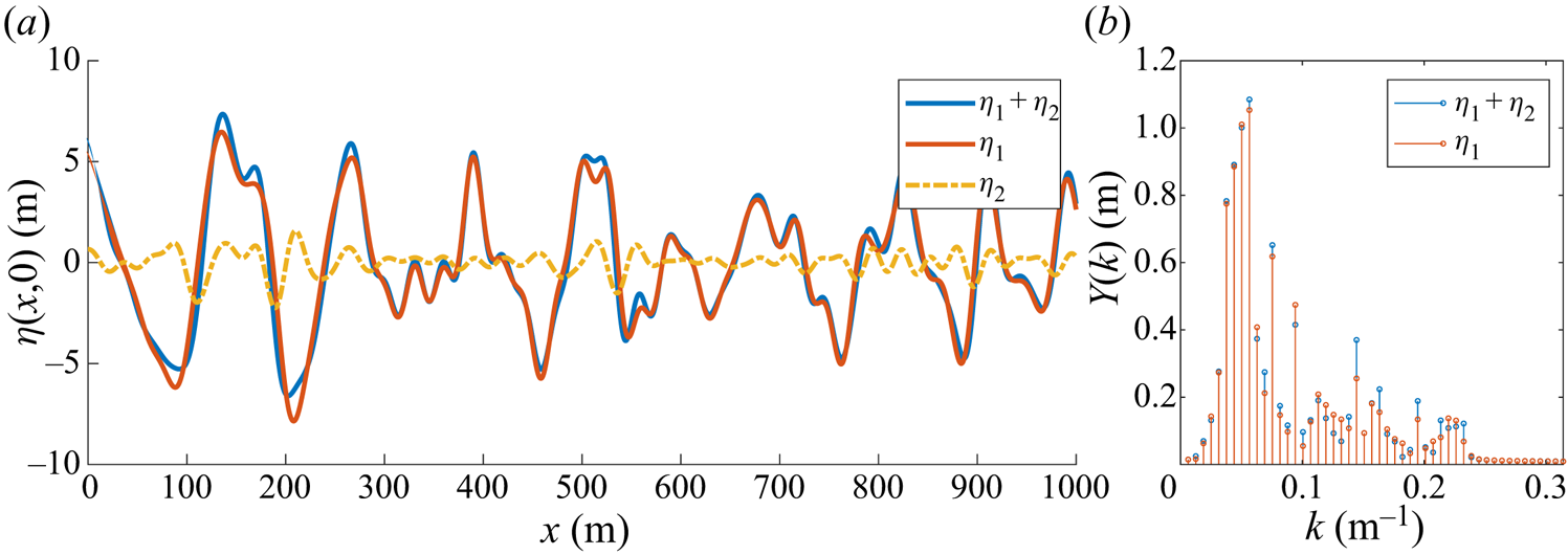
Figure 6. (a) Sea surface computed from a JONSWAP spectrum with  $\epsilon =0.2$ (see table 1):
  $\eta _1$ (red curve) depicts free waves only;
  $\eta _2$ (yellow dash-dotted curve) depicts bound waves only; and
  $\eta _1+\eta _2$ (blue curve) depicts the free surface with free and bound waves. (b) Fourier amplitude spectra of
  $\eta _1$ and
  $\eta _1+\eta _2$.
The presence of bound modes presents a difficulty for forecasting, since part of the measured energy does not propagate with the expected dispersion relation. Figure 6(b) shows Fourier amplitude spectra of all modes  $\eta _1+\eta _2$, as well as of the free modes
  $\eta _1$ only. Only the latter propagate in accordance with linear or weakly nonlinear dispersion (3.2), depending on the forecasting model used. Nevertheless, the measurement procedure outlined in § 3.1 perforce identifies all of the mode amplitudes (as shown in blue in figure 6b) as free modes.
Given an ensemble of well-resolved spatio-temporal measurements, it is possible to construct a wavenumber–frequency spectrum  $\varPsi ({k},\omega )$ without assuming the linear dispersion relation. Energy that does not fall on the curved plane
  $\omega = \sqrt {g|k|}$ in spectral
  $({k},\omega )$ space can then be attributed to bound waves or, for field measurements, ambient currents. For surface elevation measurements at a single time, by contrast, it is theoretically impossible to distinguish free and bound modes. The smallness of the second-order bound mode contributions means that they do not give rise to appreciable errors in forecasting if the wave steepness is low. In a practical setting, a measurement contains free as well as bound modes, like the blue curve
  $\eta _1+\eta _2$ in figure 6(a).
The sea state in figure 7 is computed from a JONSWAP spectrum with  $\epsilon =0.2$ (see table 1), which is evolved as described in § 2.1, with bound waves added from the analytical expression (2.7). Two forecasts based on measurements at
  $N=200$ points over
  $L=1000\ \textrm {m}$ are contrasted. Forecast
  $\zeta _Z$ (red solid curve) simply applies the procedures of § 3.1 to the measurements, ignoring the fact that bound modes are present in the sea. It thereby misidentifies the bound mode energy as belonging to free modes (see figure 6b). All modes in this forecast
  $\zeta _Z$ are evolved using the Zakharov equation forecast (3.7). By contrast, the second forecast
  $\tilde {\zeta }_Z$ (yellow dashed curve) presents an ideal situation that cannot be realized in practice: it uses a fabricated measurement of the free waves only at
  $t=0\ \textrm {s}$, which is evolved to
  $t=60\ \textrm {s}$ using (3.7) and (3.8), with the analytical bound modes then added from (2.7). It differs from the sea state through its use of fewer modes obtained from the measurements.
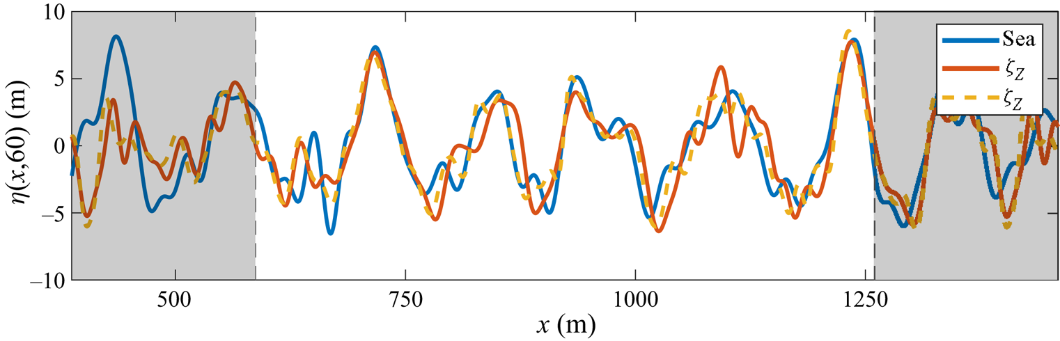
Figure 7. Comparison of a sea (blue curve, containing free and bound modes  $\eta _1 + \eta _2$) generated using a JONSWAP spectrum with
  $\epsilon =0.2$ and two forecasts at time
  $t=60\ \textrm {s}$. (Red solid curve) Forecast assuming all modes are free and evolving in time using the Zakharov equation via (3.7) and (3.8). (Yellow dashed curve) Forecast based on identifying the free modes at the measurement time (see red Fourier amplitudes in figure 6b), evolving these in time using the Zakharov equation, and adding the analytical bound modes calculated using (2.7) at
  $t=60\ \textrm {s}$.
In figure 7 it is difficult to distinguish the error incurred by an inability to accurately identify bound mode contributions from that inherent in forecasting a highly nonlinear sea from a limited number of measurements. As noted previously, the forecast quality depends on the measurement area  $L$ and the waves therein for a particular realization of the sea surface. Table 3 considers averages over 50 realizations at a variety of forecast times (
 $t=30,\ 60$ and 90 s) and average wave slopes (JONSWAP spectra with
  $\epsilon =0.1,\ 0.15$ and 0.2). It compares the average correlation in the predictable region of
  $x$-space between sea and either the forecast
  $\zeta _Z$ (where bound modes are misidentified as free), or the forecast
  $\tilde {\zeta }_Z$ (an ideal scenario where bound and free modes can be distinguished in the measurement at
  $t=0\ \textrm {s}$).
Table 3. Mean correlation over 50 realizations between a sea with bound waves and a forecast that fails to account for bound modes  $\zeta _Z$, or an artificial forecast that employs analytical bound modes for the measurement
  $\tilde {\zeta }_Z$. The sea is initialized from a JONSWAP spectrum with
  $\epsilon =0.1,\ 0.15$ and
  $0.2$ (see table 1), and comparisons are presented at times
  $t=30,\ 60$ and
  $90\ \textrm {s}$.
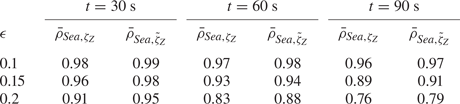
The mean correlation for the ideal forecast  $\bar {\rho }_{Sea,\tilde {\zeta }_Z}$ compares favourably with that seen for
  $\bar {\rho }_{Sea,\zeta _Z}$ in table 2, where bound modes were not considered. For waves of low to moderate steepness with
  $\epsilon =0.1$ and 0.15, the differences between
  $\zeta _Z$ and
  $\tilde {\zeta }_Z$ are rather small, and the forecasting error introduced by the bound waves is minimal. For steeper waves, however, the differences are somewhat more marked, particularly for long forecasting times.
4.4. Comparison with HOS simulations
In order to validate our approach, and study the effects of higher-order nonlinearities, the three forecasting approaches can also be applied to reference seas generated by means of HOS simulations. In this section, we employ the open-source HOS-Ocean solver (Ducrozet et al. Reference Ducrozet, Bonnefoy, Le Touzé and Ferrant2016) to generate and propagate wave fields in a two-dimensional domain. HOS order  $M=5$ is chosen to include higher-order nonlinearities beyond those captured by the Zakharov equation, and a JONSWAP spectrum with
  $\gamma =5$,
  $k_p=0.05\ \text {m}^{-1}$ and
  $H_s$ as in table 1 is used to generate the initial wave field in deep water.
Each initial wave field (at  $t=0\ \textrm {s}$) is sampled at
  $S=300$ uniformly distributed points over a length of
  $L=2000\ \textrm {m}$. The initial wave field is subsequently evolved in time with HOS (the details of which may be found in Ducrozet et al. (Reference Ducrozet, Bonnefoy, Le Touzé and Ferrant2007, Reference Ducrozet, Bonnefoy, Le Touzé and Ferrant2016) and Bonnefoy et al. (Reference Bonnefoy, Ducrozet, Le Touzé and Ferrant2010)), while the sampled points are used to generate forecasts using linear dispersion, nonlinear dispersion or the Zakharov equation. One realization of the sea is compared to the three forecasts at
  $t=60\ \textrm {s}$ in figure 8 for
  $\epsilon =0.1,\ 0.15$ and
  $0.2$ (see table 1). For low steepness (
 $\epsilon =0.1$) all forecasts provide good agreement, and up to moderate steepness (
 $\epsilon = 0.15$) both nonlinear forecasts
  $\zeta _S$ and
  $\zeta _Z$ perform very well. For yet steeper waves, the mismatch between sea and
  $\zeta _S$ and
  $\zeta _Z$ is similar in scale to that seen in figure 3.
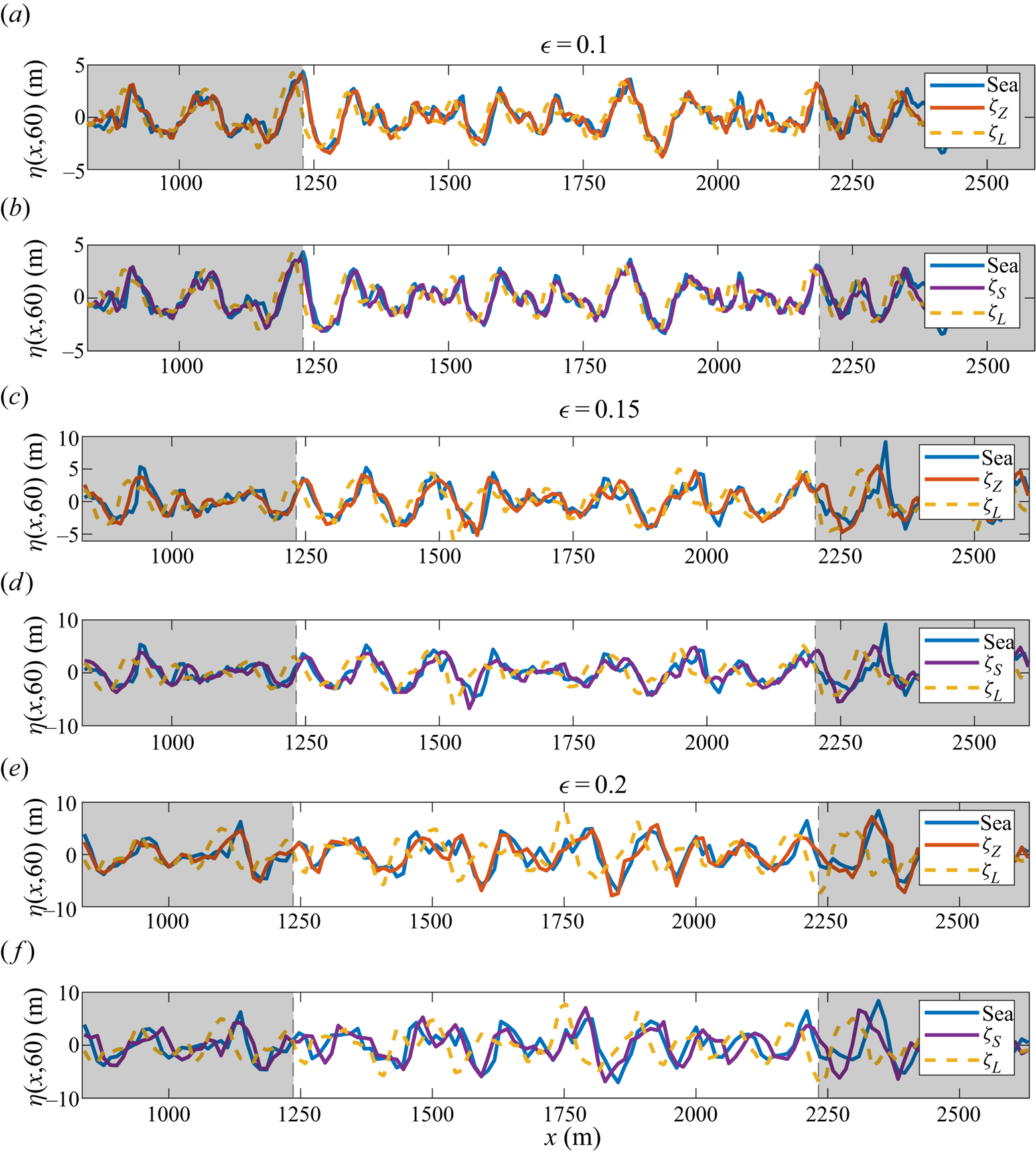
Figure 8. Comparison of forecasts with a reference sea propagated via HOS (blue solid line, denoted ‘Sea’) at  $t=60\ \textrm {s}$, for
  $\epsilon = 0.1$ (a,b),
  $\epsilon =0.15$ (c,d) and
  $\epsilon =0.2$ (e,f). (a,c,e) The sea is compared to a linear forecast (yellow dashed line) and a forecast based on the Zakharov equation (red solid line). (b,d,f) The sea is compared to a linear forecast (yellow dashed line, as in a,c,e) and a linear forecast with nonlinear frequency correction (purple solid line).
Since each realization of the sea employs uniformly distributed random phases, an aggregate measure of the quality of the three forecasting approaches for HOS-generated sea surfaces (denoted ‘Sea’) is provided by the mean correlations shown in table 4. The mean correlations are comparable to those found in table 2, where the reference sea is generated from the Zakharov equation, as can be seen by comparing the number of forecasts marked bold (with mean correlation greater than or equal to 0.8, to indicate a good match) in either table. Comparison with HOS simulations of order  $M=3$ show no appreciable difference from those with
  $M=5$ presented in table 4, underscoring the relatively small contributions of these higher-order terms on the scales involved.
Table 4. Mean correlation between a sea simulated with HOS and forecasts for  $t=30,\ 60$ and
  $90\ \textrm {s}$, with
  $\epsilon =0.1,\ 0.15$ and
  $0.2$. In each instance, 50 realizations of the reference ocean surface and corresponding forecasts are employed, and the mean correlation over the predictable interval is calculated. Mean correlations
  $\geq 0.8$ have been marked bold.
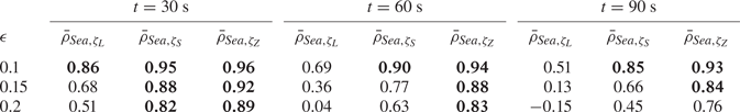
5. Conclusions
We have introduced and developed a deterministic wave forecasting methodology based on the Zakharov equation, and used it to investigate the effect of nonlinearity and bound waves on wave forecasts. The Zakharov equation readily yields analytical insight, and the present approach is complementary to recent work employing the higher-order spectral method for reconstruction of nonlinear wave fields (see recent work by Köllisch et al. (Reference Köllisch, Behrendt, Klein and Hoffmann2018), Qi et al. (Reference Qi, Wu, Liu, Kim and Yue2018a) and Desmars et al. (Reference Desmars, Bonnefoy, Grilli, Ducrozet, Perignon, Guérin and Ferrant2020)).
Under an assumption that all interactions take place close to a central wavenumber, the nonlinear Schrödinger equation and its extensions may be derived from the Zakharov equation (2.3) (see Stiassnie Reference Stiassnie1984). The Zakharov equation thus generalizes the nonlinear Schrödinger models, which have been widely used to study rogue waves (Onorato & Suret Reference Onorato and Suret2016), as well as in recent studies of wave forecasting (see e.g. Trulsen Reference Trulsen2005; Simanesew et al. Reference Simanesew, Trulsen, Krogstad and Nieto Borge2017; Klein et al. Reference Klein, Dudek, Clauss, Ehlers, Behrendt, Hoffmann and Onorato2020). Because of its lack of bandwidth restrictions, our method is applicable to both narrow JONSWAP spectra (as in § 4.1) as well as broad PM spectra (as in § 4.2).
Nonlinear effects can play an important role in deterministic wave forecasts, the extent of which is dependent on both average steepness as well as forecasting time. For small wave slopes below  $\epsilon =0.1$, linear theory is sufficient to provide forecasts for moderately long time – up to approximately
  $10T_p$, for
  $T_p$ the peak wave period of the spectrum. Nevertheless, the weakly nonlinear corrections associated with finite-amplitude effects – analogues of Stokes’ frequency correction – can be easily and effectively computed from the sea-surface measurements, and yield a marked improvement over linear forecasts.
For moderately nonlinear wave fields, up to  $\epsilon =0.15$, such third-order frequency corrections are likely to be sufficient to provide accurate forecasts, as very little energy exchange between modes can occur within the predictable time frame. For steeper wave fields, the full Zakharov equation should be brought to bear to obtain an accurate forecast. While the theoretical time scale of the Zakharov equation is
  $t_2 \sim \epsilon ^{-2} T_p$, our results indicate that departures from linear theory begin to appear at
  $t_1 \sim \epsilon ^{-1} T_p$, which must be taken into account when preparing a forecast. For the time scales involved in deterministic forecasting, the energy exchange captured by the cubic nonlinearities of the Zakharov equation is sufficient, as demonstrated by comparisons with HOS of order five in § 4.4.
The Zakharov formulation yields an analytical expression for the second- and higher-order bound waves. Bound waves are present in the wave field as a consequence of the harmonic description of nonlinear wave motion, and thus do not obey the natural dispersion relation. When sampling a real sea surface at a number of points, the associated Fourier amplitudes will contain such bound mode contributions in addition to free waves. By including appropriate bound modes in the generated reference sea, it is possible to assess the effect of this misidentification of bound wave energy. For the cases considered, with steepness up to  $\epsilon =0.15$, second-order bound modes form a relatively minor contribution. Future work will be devoted to accurate identification of bound waves from a wave record, with a view towards furnishing more accurate forecasts for longer times and highly nonlinear seas.
While this work has examined the simplest case of unidirectional propagation, subsequent studies will consider directionally propagating waves from the perspective of the Zakharov equation. In the first instance, this will impact the geometry of the predictable region, thereby altering the linear forecast. As shown by Stuhlmeier & Stiassnie (Reference Stuhlmeier and Stiassnie2019), the extent of the nonlinear frequency correction is also direction-dependent, giving rise to a complex interplay between wave frequency, amplitude and direction in determining the forecast. The inclusion of local wind and a suitable representation of wave breaking – via forcing terms in the Zakharov equation (see Annenkov & Shrira Reference Annenkov and Shrira2009) – would further present an opportunity for comparison with experiments.
Acknowledgements
The authors are grateful for helpful comments and suggestions of the referees on earlier drafts of this paper.
Funding
M.S. is grateful for the support of the Israel Science Foundation, grant 261/17.
Declaration of interests
The authors report no conflict of interest.


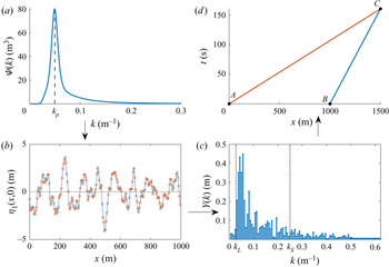


 Open access