


1. Introduction
Most of the glacierized regions in the world have experienced glacier wastage over the last several decades due to warming trends (IPCC, Reference Pörtner, Roberts, Masson-Delmotte, Zhai, Tignor, Poloczanska, Mintenbeck, Nicolai, Okem, Petzold, Rama and Weyer2019). A recent Hindu Kush-Himalaya (HKH) Assessment claimed that even if global warming is constrained to the most ambitious target of 1.5°C (2015 Paris Agreement), at least ~30% of the permanent glacier cover in the HKH region is destined to meltdown within this century, leaving behind ~2 billion people in peril (Bolch and others, Reference Bolch, Wester, Mishra, Mukherji and Shrestha2019). Although glaciers are declining in the Himalayan ranges (Azam and others, Reference Azam2018), the glaciers in Karakoram, Kunlun Shan and Pamir stand out as stable or advancing (Hewitt, Reference Hewitt2005; Yao and others, Reference Yao2012; Brun and others, Reference Brun, Berthier, Wagnon, Kääb and Treichler2017; de Kok and others, Reference de Kok, Tuinenburg, Bonekamp and Immerzeel2018; Kumar and others, Reference Kumar2019; Farinotti and others, Reference Farinotti, Immerzeel, de Kok, Quincey and Dehecq2020). These contrasting signals are difficult to interpret in terms of climate, as meteorological measurements at glaciated catchments and higher altitudes are difficult and often sparse (Fowler and Archer, Reference Fowler and Archer2006; Shekhar and others, Reference Shekhar, Chand, Kumar, Srinivasan and Ganju2010; Dimri and Dash, Reference Dimri and Dash2012). Initial investigations suggest that local irrigation-derived evapotranspiration (de Kok and others, Reference de Kok, Tuinenburg, Bonekamp and Immerzeel2018) and snowfalls (Bonekamp and others, Reference Bonekamp, de Kok, Collier and Immerzeel2019; Kumar and others, Reference Kumar2019) control the regional differences in glacier response in the HKH region. However, a complete understanding requires more in situ, high-altitude meteorological and glaciological observations (Azam and others, Reference Azam2018; Bolch and others, Reference Bolch, Wester, Mishra, Mukherji and Shrestha2019; Litt and others, Reference Litt2019; Farinotti and others, Reference Farinotti, Immerzeel, de Kok, Quincey and Dehecq2020). Thus, the dearth of primary in situ dataset is a major concern when it comes to assessing social and economic impacts of the Himalayan glaciers on the inhabited downstream regions (IPCC, Reference Pörtner, Roberts, Masson-Delmotte, Zhai, Tignor, Poloczanska, Mintenbeck, Nicolai, Okem, Petzold, Rama and Weyer2019; Pritchard, Reference Pritchard2019).
To date, only 24 glaciers covering fewer than 1% of the total glacierized area in the Himalayan region have been monitored in the field using the glaciological method, most of them being from India. The mean mass balance for 24 Himalayan glaciers was estimated to be −0.59 m w.e. a−1 between 1975 and 2015 (Azam and others, Reference Azam2018). Glaciological mass-balance measurements are challenging in the Himalayan region due to the vast glacierized area, extreme altitudes and climate, rough terrain as well as trans-boundary problems. Nonetheless, several new mass-balance measurement programmes in the Indian, Nepalese and Bhutanese Himalaya have begun in recent years (Ramanathan, Reference Ramanathan2011; Tshering and Fujita, Reference Tshering and Fujita2016; Sherpa and others, Reference Sherpa2017; Soheb and others, Reference Soheb2020).
Due to the increased availability of high-resolution satellite imageries in recent years, several geodetic glacier mass-balance studies have been conducted in the Lahaul-Spiti region (>2000 km2 of glacierized area; Vincent and others, Reference Vincent2013) in the western Himalaya. A geodetic mass balance of −0.36 ± 0.1 m w.e. a−1 over 1999–2013 was reported for the Lahaul-Spiti region (Mukherjee and others, Reference Mukherjee, Bhattacharya, Pieczonka, Ghosh and Bolch2018). Another study estimated similar mass loss of −0.37 ± 0.09 m w.e. a−1 over 2000–2016 (Brun and others, Reference Brun, Berthier, Wagnon, Kääb and Treichler2017). These estimates are similar to the geodetic mass balance of −0.37 m w.e. a−1 over 1962–2015 for the whole Himalayan Range (Azam and others, Reference Azam2018). Shekhar and others (Reference Shekhar, Chand, Kumar, Srinivasan and Ganju2010) conducted an extensive analysis of in situ air temperature and precipitation data from the higher altitude stations in western Himalaya since the 1980s. They reported a substantial winter temperature rise and snowfall decline, possibly responsible for the observed glacial mass loss in the western Himalaya including Lahaul-Spiti region.
Current glacier mass loss in the region is accompanied by considerable surface thinning, even at higher altitudes (Azam and other, Reference Azam2012; Brun and others, Reference Brun, Berthier, Wagnon, Kääb and Treichler2017) and a reduction of surface ice velocity (Garg and others, Reference Garg, Shukla, Tiwari and Jasrotia2017; Dehecq and others, Reference Dehecq2019). However, these velocity reductions are often remotely sensed due to non-availability of in situ measurements in the Lahaul-Spiti region and are inadequate for clearing the ambiguity regarding the glacier surface mass-balance response to the ice velocity. Surface ice velocity measurements in other parts of the Himalaya are also rare.
Hydrological investigations are also important for understanding glacier response to current climatic conditions as the variability in meltwater discharge mainly depends on regional meteorology. No study was conducted to investigate the relationship of discharge with various meteorological variables in the Lahaul-Spiti region, except for a few recent model-based studies (Engelhardt and others, Reference Engelhardt2017; Azam and other, Reference Azam2019). Compared to western Himalaya, glaciers in central Himalaya's Garhwal region were well investigated in the context of local meteorology and hydrology (Thayyen and others, Reference Thayyen, Gergan and Dobhal2005; Thayyen and Gergan, Reference Thayyen and Gergan2010; Singh and others, Reference Singh, Kumar and Kishore2011). This lack of hydro-meteorological data from small glacier catchments is a major concern while validating large-scale glacio-hydrological models (Azam and other, Reference Azam2018; Bolch and others, Reference Bolch, Wester, Mishra, Mukherji and Shrestha2019; Li and others, Reference Li2019).
Changes in glacier mass balance, surface ice velocity and stream discharge are related to prevailing meteorological conditions (Fischer, Reference Fischer2011). Therefore, long-term mass-balance observations together with hydro-meteorological measurements are the utmost requirement for assessing climate change and understanding the climate–glacier relationships in the Himalaya. The present study is focused on filling these data gaps and presents extensive results of meteorology, mass balance, surface ice velocity and discharge measurements in the Chhota Shigri Glacier (western Himalaya). The key objectives of this study are: (1) study the annual (B a), winter (B w) and summer (B s) glacier-wide mass balances of the Chhota Shigri Glacier during 2002–2019, (2) identify the dynamic change and adjustment in response to recent B a using field-measured surface ice velocity dataset for the period 2003–2017, and (3) present and analyse the Chhota Shigri proglacial stream discharge dataset. In addition, we also discuss the results of extensive sub-seasonal ablation measurements during 2015–2019 and two dye tracer experiments to determine the discharge time-lag characteristics of the Chhota Shigri Glacier.
2. Study area
Chhota Shigri Glacier (32.28°N, 77.58°E; Fig. 1) is located in the Lahaul-Spiti valley, western Himalaya (Himachal Pradesh, India). It is a representative (Vincent and others, Reference Vincent2013), ‘tier 2’-type (Paul and others, Reference Paul, Kääb and Haeberli2007) glacier and has been studied for various aspects such as mass balance, energy balance, dynamics, ice thickness and hydrology (Azam and others, Reference Azam2012, Reference Azam2014a, Reference Azam2016, Reference Azam2019). Chhota Shigri catchment covers an area of 34.7 km2 at its outlet (discharge station at ~3840 m a.s.l. shown in Fig. 1) (Wagnon and others, Reference Wagnon2007). The total glacierized area in this catchment is 16.1 km2, of which Chhota Shigri Glacier covers 15.5 km2 while the remaining 0.6 km2 is covered by a few small hanging glaciers (Azam and others, Reference Azam2016). The glacier is ~9 km long with an altitude range of ~4072–5830 m a.s.l. with ice surface slopes ranging between 10 and 45°. The snout of this glacier is well defined, lying in a narrow valley and giving birth to a single proglacial stream feeding Chandra River, one of the tributaries of Chenab River (Fig. 1). Chhota Shigri Glacier is a valley-type, non-surging, temperate and mostly clean glacier. This glacier is oriented roughly north-south in its ablation area and has different aspects in the accumulation area. A recent study reported that debris cover has increased from 3.4% (0.53 km2) in 2005 (Vincent and others, Reference Vincent2013) to ~11% (1.8 km2) in 2014 (Garg and others, Reference Garg, Shukla, Tiwari and Jasrotia2017). The total stored ice volume of the Chhota Shigri Glacier in 2013 was estimated to be 1.74 ± 0.25 km3 using GlabTop2 Model (Ramsankaran and others, Reference Ramsankaran, Pandit and Azam2018). In summer, the glacier receives precipitation through Indian Summer Monsoon (ISM) and in winter through Western Disturbances (WDs). A list of geographical and topographical attributes of the Chhota Shigri Glacier is given in Table 1.

Fig. 1. The left panel shows the location of the Chhota Shigri Glacier in Himachal Pradesh in the western Himalaya (India). The locations of Bhuntar, Manali, Koksar and Gondhla meteorological stations, glacier cover (RGI Consortium, 2017) as well as the orographic barrier, are also shown (background: SRTM DEM with hill shade effect). Location of the Chhota Shigri Glacier (red dot) in Indian boundary is also shown. The right panel is the close-up view showing the catchment of the Chhota Shigri Glacier (background: ASTER L1T acquired on 21 September 2017) and the glacier area (black outline). The location of ablation stakes on the debris-cover area (black dots), eastern flank (blue dots), western flank (green dots), accumulation measurement sites (orange squares), discharge measurement site (red dot), AWS-BC (at base camp; blue star), AWS-M (on lateral moraine; red star) and Geonor automatic precipitation gauge (at base camp; turquoise triangle) are also shown.
Table 1. Geographical and topographical attributes of Chhota Shigri Glacier

a Garg and others (Reference Garg, Shukla, Tiwari and Jasrotia2017).
b Ramsankaran and others (Reference Ramsankaran, Pandit and Azam2018).
3. Data and methodology
3.1 Meteorological data
Meteorological data were recorded to understand the long-term climate setting of the glacier and to define the inter-linkages with mass balance and discharge. Meteorological variables such as air temperature (T air), relative humidity (RH), wind speed (u), incoming and outgoing short-wave (S in and S out) and incoming and outgoing long-wave (L in and L out) radiations were recorded since August 2009 at the automatic weather station located off-glacier on a lateral moraine (hereafter AWS-M; 4863 m a.s.l.) of the Chhota Shigri Glacier (Fig. 1). AWS-M provides one of the longest meteorological data series at such high altitudes. However, there is a gap between 22 February 2015 and 2 October 2016 (589 d) when the AWS-M could not record meteorological data during night time, due to disconnected wire between the solar panel and the battery. Meteorological variables were sampled at 30 s frequency and recorded as 30 min averages by a Campbell CR1000 data logger. Sensor specifications of AWS-M and data treatment steps are provided in Azam and others (Reference Azam2014a). Precipitation (P) was recorded since July 2012 at the base camp through an all-weather precipitation gauge (Geonor T-200B), which employs a weighing device to measure liquid and solid precipitation (Fig. 1). Due to the battery failure of Geonor gauge in 2013/14, we used daily P data from the IMD-gridded (Indian Meteorological Department) dataset from the nearest grid. No correction was added to the IMD-gridded dataset, as mean precipitation from Geonor already matches roughly with IMD data over 2012–2016 (965 vs 1232 mm a−1).
3.2 Glaciological mass-balance measurements
3.2.1 Point to annual glacier-wide mass balance
Point mass-balance measurements were conducted to calculate the glacier-wide mass balance of the Chhota Shigri Glacier. Mass-balance measurements have been carried out since 2002 (Wagnon and others, Reference Wagnon2007; Ramanathan, Reference Ramanathan2011). In this study, we present mass balance since 2014. Mass-balance values before 2014 can be accessed from Azam and others (Reference Azam2016). The hydrological year is defined from 1 October to 30 September of the following year on this glacier, mainly for practical reasons, since access to the glacier after 15 October is restricted (Azam and others, Reference Azam2016).
B a is calculated following standard glaciological protocol (Kaser and others, Reference Kaser, Fountain and Jansson2003). The ablation was measured through a well-distributed network of ~22 bamboo stakes (inserted up to 8–10 m deep in the ice) distributed between 4300 and 4900 m a.s.l., whereas the net annual accumulation was obtained in the accumulation area between 5150 and 5550 m a.s.l at six sites (sometimes four/five) depending on accessibility, by drilling snow cores or pits (Fig. 1). In the accumulation area, the number of measurement sites is limited because of difficult access and harsh climatic conditions. The densities were estimated from snow cores in the accumulation zone. In the mass-balance calculation, ice density was assumed to be 900 kg m−3, and in the presence of snow, the density was systematically measured in the field or assumed as 350 kg m−3 for the ablation zone.
In October 2015, due to difficult access (dense crevasses), no suitable accumulation measurements were carried out above 5100 m a.s.l. on both the eastern and western flanks. Only two accumulation drills were carried out at lower altitudes (5050 and 5100 m a.s.l.) on the western flank. Since the measurements at 5050 and 5100 m a.s.l. were not sufficient to calculate the B a, accumulation at representative locations was estimated from three representative years (2010/11, 2011/12 and 2013/14) where the root mean square error (RMSE) of mean altitudinal mass balance in the ablation area was least with reference to 2014/15. Measured mean accumulations of 2010/11, 2011/12 and 2013/14 at different point locations were applied to the final mass-balance calculation for 2014/15. In September 2018, the glacier was inaccessible due to heavy snowfalls that blocked the only access for rest of the summer season and no field measurements could be carried out. For 2017/18, annual ablation was computed from the stake measurements of 15 September 2018. Since the whole valley was entirely covered by thick snow cover, we assumed that there was negligible melting between 15 and 30 September and minimal effect on B a. The same approach as for 2014/15 was applied in accumulation estimates for 2017/18, where 2003/04, 2005/06 and 2012/13 were found to be the least RMSE years. Precipitation measurements at base camp suggested a total of 169 mm w.e. snowfall between 22 and 24 September 2018. We also included this snowfall amount to the annual accumulation of 2017/18 by applying a precipitation gradient of 0.1 m km−1 (Azam and others, Reference Azam2014b).
The hypsometry of the Chhota Shigri Glacier used for B a calculation is computed using a DEM derived from Pléiades images from 18 August 2014 (Azam and other, Reference Azam2016).
3.2.2 Sub-seasonal ablation measurement
The stake network was monitored regularly in order to estimate the sub-seasonal ablation rates and to understand the control of debris cover at different altitudes. Since 2015, measurements were performed every ~7 d interval at all visible stakes between 4350 and 4900 m a.s.l. except in 2018 and 2019, when the interval was ~10 d or more. Several data gaps exist in every year's record due to issues such as bad weather conditions, broken stakes, delay in re-installing melted-away stakes, stakes buried in snow, etc. Finally, we have 157, 203, 187, 80 and 58 datasets in 2015, 2016, 2017, 2018 and 2019, respectively, of which 22, 26, 28, 12 and 8 are from the debris-covered zone.
3.2.3 Uncertainty in the annual glacier-wide mass balance
The overall error in B a may come from various type of sources, such as ice/snow density, core length, stake height determination, liquid-water content of the snow, snow height, surface area delineation, hypsometry, etc. Applying these errors at different altitudinal ranges, the uncertainty in B a was calculated as ±0.40 m w.e. a−1, which comes from a variance analysis by Thibert and others (Reference Thibert, Blanc, Vincent and Eckert2008). The error estimation details are provided in Azam and others (Reference Azam2012).
3.3 Surface ice velocity
The surface ice velocity measurements were conducted to define the current state of the glacier as a response to climate change. Annual surface ice velocities were measured at the end of the ablation period (September) on the Chhota Shigri Glacier by determining the displacement of the stakes using a Differential Global Positioning System (DGPS). A Topcon DGPS was used until 2015, followed by a dual-frequency Leica device (1 s acquisition frequency, ~30 s to 1 min acquisition time at every stake) to measure the stakes. In 2016/17, only four stakes were surveyed due to early snowfall at the end of the ablation period that covered most of the stakes. Also, in 2018, no measurements were performed due to inaccessible way up to the glacier (heavy snowfall, discussed in Section 3.2.1). Since no measurements were carried out in 2014 (due to unavailability of DGPS), we calculated the velocities between 2013 and 2015 (Section 4.7). The DGPS measurements were performed in kinematic mode relative to two fixed reference points (one at the base camp at 3844 m a.s.l. and another at 4804 m a.s.l. in the upper ablation area) outside of the glacier on firm rocks. Accuracy of DGPS measurements depends on several factors such as the number of operating satellites, their geometrical configuration in the sky, the distance to the DGPS base station and the acquisition frequency and duration (Wagnon and others, Reference Wagnon2013). Surface ice velocities measured from stake displacements have an accuracy of ~0.3 m a−1 (Azam and others, Reference Azam2012).
3.4 Discharge measurement
Discharge measurements were carried out at the Chhota Shigri catchment outlet during the ablation seasons between 2010 and 2016 (Fig. 1 and Fig. S1 in Supplementary Materials). Observations were subject to glacier access (the road is not always clear/accessible after winter snow/landslides) and therefore not always possible for the entire summer. The discharge is very low in the Chhota Shigri catchment during October/November as revealed by modelling (Azam and others, Reference Azam2019). The gauging site was chosen at a distance of ~2 km downstream from the glacier terminus as it was straight with single channel having low turbulence. No other stream joins upstream of the gauging site, and it is assumed that the discharge measured during the study period is from glacier ice and snowmelt, and precipitation if any. Discharge measurements were performed using the velocity-area method. A graduated staff gauge was installed at the gauging site for manual monitoring of water level, while an automatic water level recorder (OTT Orpheus Mini; accuracy ±0.05%) was also installed at the gauging site for continuous recording (30 min interval) of water level variation. Dipsticks were used for measurements of the cross-section area of the meltwater channel twice a year (June and September/October). In May 2010, depth-integrated velocity measurements were performed with a current meter, and an initial rating curve was established for the conversion of water levels into discharge, which was updated with frequent water velocity measurements using wooden floats throughout the studied period. In 2016, there were no automatic measurements of water level due to the malfunctioning of the water level recorder. Therefore, the final daily discharge was calculated using only manual stage height and float measurements (twice a day: 08:00 and 18:00 h). There is often considerable uncertainty associated with the volumetric measurement of flowing water due to the technical limitations of measuring equipment, techniques, feasibility, etc. (Frenierre and Mark, Reference Frenierre and Mark2014). Since the bottom of Chhota Shigri stream is not paved and difficult to keep free from the boulders transported through water, particularly in the peak melt period (July and August) and other technical and instrumental limitations, the possibility of error in discharge measurements is expected to be ~25% of the total discharge (Eeckman and others, Reference Eeckman2017).
3.5 Dye tracer experiment
In August 2016, dye tracer experiments were carried out by injecting known quantities of rhodamine B dye into two different moulins in the lower ablation zone (LAZ) of the glacier. This dye was chosen as the tracer because it has been used successfully in glaciers around the world to delineate sub-glacial hydrology and is non-toxic at parts per billion (ppb) levels (Pottakkal and others, Reference Pottakkal2014). Dye emergence was detected and logged at each second by a Turner Designs model 10-AU Continuous Flow Field Fluorometer at the discharge site.
4. Results
4.1 Ten-year meteorological measurements (2009–2019) at 4863 m a.s.l.
Figure 2 shows monthly variations in T air, RH, u, S in, S out, L in and L out between 1 October 2009 and 28 September 2019 recorded at the AWS-M (4863 m a.s.l.). To present an interannual comparison, four seasons were categorized following Azam and others (Reference Azam2014a): post-monsoon (October–November), winter (December–March), pre-monsoon (April–May) and summer-monsoon (June–September). A summary of the seasonal and annual values of different variables is presented in Table S1.

Fig. 2. Mean monthly values of u (blue dots), RH (green dots), T air (red dots), S in, S out, L in and L out (black and grey bars) recorded at AWS-M (4863 m a.s.l.) for the 2009/10 to 2018/19 hydrological years. Error bars (standard deviation; SD) were computed using monthly values of each year (n = 10). P (bottom panel) from Chhota Shigri base camp measured using Geonor all-weather gauge (2012–2018; with a gap from October 2013 to September 2014), whereas long-term Bhuntar (1092 m a.s.l.; ~50 km from Chhota Shigri), Manali (1950 m a.s.l.; 30 km) and Koksar (3204 m a.s.l.; 35 km) datasets were collected from Indian Meteorological Department (IMD) and Gondhla (3144 m a.s.l.; 55 km) dataset was obtained from Global Historical Climatology Network (GHCN).
In summer, mean monthly T air ranges from 1.9 to 4.3°C, corresponding to a 10-year summer mean T air of 2.8°C. Daily mean T air remains positive during the summer with a cumulative positive degree day (CPDD) (∑T air+) of 378.3°C, which corresponds to 98% of the annual CPDD during the study period (Table S1). Mean S in is high (323 W m−2) during the summer. RH is highest in summer at 67%, corresponding to the highest mean values of L in (281 W m−2) owing to the frequent overcast sky. Mean u is lowest in summer at 2.8 m s−1. In winter, with a very high u of 5.4 m s−1, the air is comparatively drier (RH = 40%) and colder (T air = −12.9°C). Daily mean T air, therefore, does not go above freezing point. S in and L in are the lowest, corresponding to a mean of 203 and 198 W m−2 throughout the entire winter season.
Pre-monsoon is characterized by a progression of ISM onset, with a gradual increase in T air, RH and L in and a decrease in u. S in is highest in the pre-monsoon (374 W m−2). In contrast, post-monsoon begins with a sudden drop in T air. RH, S in and L in start to decrease slowly, whereas u sharply increases about twofold compared to summer (4.3 m s−1), all of which demonstrate the transition of seasons and onset of winter (Shea and others, Reference Shea2015).
The annual temperature lapse rare (TLR) for the Chhota Shigri catchment was found to be 6.16°C km−1, calculated using two AWSs. The calculated TLR is close to the environmental lapse rate (6.5°C km−1) (Fig. S2).
Figure 2 (bottom panel) shows the monthly P for five complete hydrological years between October 2012 and September 2018 (with a gap from October 2013 to September 2014) at Chhota Shigri Glacier base camp (3850 m a.s.l.). Winter seasons are the wettest when presumably most of the contributions come as solid precipitation (128 mm month−1) followed by pre-monsoon (100 mm month−1), summer (43 mm month−1) and post-monsoon (19 mm month−1) corresponding to an annual sum of 922 mm (Table S1). To understand the regional P distribution, we focus on the P at neighbouring stations, also plotted in Figure 2 (bottom panel). Monthly P of these stations exhibits a large spatial variability even though located within a 50 km radius of the study area (Fig. 1), due to altitude differences and an orographic barrier restricting moisture flow of ISM into the leeward side (Fig. 1). Overall, on the windward side (Bhuntar and Manali stations), July and August are the most active and wettest months, whereas on the leeward side (Chhota Shigri, Koksar and Gondhla stations), precipitation peaks in February and March. On a seasonal scale, windward side stations received slightly higher precipitation in summer than in winter (51 and 58% in summer and 49 and 42% in winter at Bhuntar and Manali, respectively) suggesting ISM dominance, while leeward side stations received significantly higher P in winter (46, 41 and 33% in summer and 54, 59 and 67% in winter at Koksar, Gondhla and Chhota Shigri, respectively) signifying the dominance of WDs in the Lahaul-Spiti region. The orographic barrier and mountain range generate föhn effect during the summer-monsoon seasons when the air masses come from the south and develop a strong south-to-north gradient of P (Azam and others, Reference Azam2019).
4.2 Annual point mass balance and vertical mass-balance gradients
Figure 3a displays the annual point mass balance as a function of altitude on Chhota Shigri Glacier for five hydrological years (2014/15–2018/19). Annual point mass balances prior to 2014/15 were discussed in Azam and others (Reference Azam2016). The point mass balance on the debris-covered part is less negative despite their lower altitudes. Melting is reduced by −1 to −2 m w.e. at the lowest part of the ablation zone <4400 m a.s.l. (Fig. 3a), indicating that the debris suppresses melting by insulating the ice surface from direct solar radiation (Wagnon and others, Reference Wagnon2007). In addition, the lower part of the glacier flows into a deep and narrow valley with a south-north orientation and receives comparatively less solar radiation because of the shading effect of the steep valley walls. Thus, the ablation is reduced, and the vertical mass-balance gradient is attenuated compared to the open upper part of the glacier. A maximum point mass balance of −5.74 m w.e. was recorded at 4426 m a.s.l. on clean ice in 2015/16.
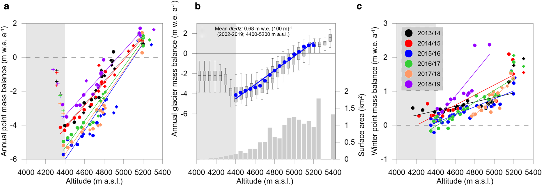
Fig. 3. (a) Annual point mass balance as a function of altitude derived from field measurements (stakes, snow cores or pits) on Chhota Shigri Glacier. Plus, circle and diamond represent the points over the debris-covered area, eastern (main glacier body) and western flank, respectively. Different colours represent point mass balances for different years. Measurement dates are given in Table S3. (b) Mean annual mass-balance (m w.e. a−1) profile between 2002/03 and 2018/19 and area-altitude (hypsometry) distribution (grey histograms). Altitudinal ranges are of 50 m (e.g. 4050 stands for the range 4050–4100 m), except for 5400 which stands for 5400–6250 m between 2002 and 2013, while it is 5400–5830 m for 2014 onwards, as the glacier area was recalculated. Calculated mass-balance gradient (db/dz) between 4400 and 5200 m (2002–2018) is shown in blue dots with the regression line. Grey shaded area is the debris-covered part (<4400 m a.s.l.). (c) Winter point mass balance as a function of altitude derived from field measurements (snow probing, cores and pits) on Chhota Shigri Glacier. Linear regression lines used to derive the winter vertical mass-balance gradient (db/dz winter), which is presented in Table 2.
Vertical mass-balance gradients (db/dz) were determined using regression lines fitted to annual point mass balance measured in the debris-free part of the glacier (main body; eastern flank) between 4400 and 5200 m a.s.l. for the period 2014/15–2018/19 for individual years (lines; Fig. 3a). The updated mean db/dz since 2002 is also estimated (blue line; Fig. 3b, Table 2). During 2002–2019, db/dz was a maximum of 0.89 m w.e. (100 m)−1 in 2017/18 whereas a minimum of 0.45 m w.e. (100 m)−1 in 2018/19 while mean db/dz was 0.68 m w.e. (100 m)−1 (SD = 0.12 m w.e. (100 m)−1). A comparison of db/dz for Himalayan glaciers is presented in Figure S3 and Table S2.
Table 2. B a, B w, B s (m w.e.), ELA (m a.s.l.), AAR (%) and db/dz (m w.e. (100 m)−1) for Chhota Shigri Glacier

The mean (in bold) and SD are also displayed for every variable. The uncertainty range for B a is ±0.40 m w.e. B a for 2002/03–2013/14 and seasonal mass balance for 2009/10–2012/13 are obtained from Azam and others (Reference Azam2016). This study: B a (2014/15–2018/19; 5 years) and seasonal mass balance (2013/14–2018/19; 6 years).
4.3 Seasonal mass balance
Figure 4 shows the B w and B s between 2009/10 and 2018/19 (this study: 2013/14–2018/19). Dates and numbers of the measurements are provided in Table S3. On Chhota Shigri Glacier, average summer ablation period lasts 96 ± 18 d from mid-June to the end of September and neither ablation nor accumulation is dominant during May–June (Azam and others, Reference Azam2014a). Since winter measurements were performed in the first week of June (±10 d), no correction was applied to the measured B w for varying measurement dates. B w, B s and vertical winter mass-balance gradients (db/dz winter) are presented in Table 2 for the studied period. Figure 3c shows the point winter mass balance measured on Chhota Shigri. Inter-annual variability of B w and B s was low (SD of ±0.28 and ±0.30 m w.e. a−1) between 2009 and 2019. The B w varied from a minimum of 0.76 m w.e. in 2012/13 to a maximum of 1.82 m w.e. in 2018/19 corresponding to a mean of 1.15 m w.e. a−1 during 2009–2019. While B s varied from a minimum of −1.78 m w.e. in 2015/16 to a maximum of −0.87 m w.e. in 2009/10 corresponding to a mean of −1.37 m w.e. a−1.
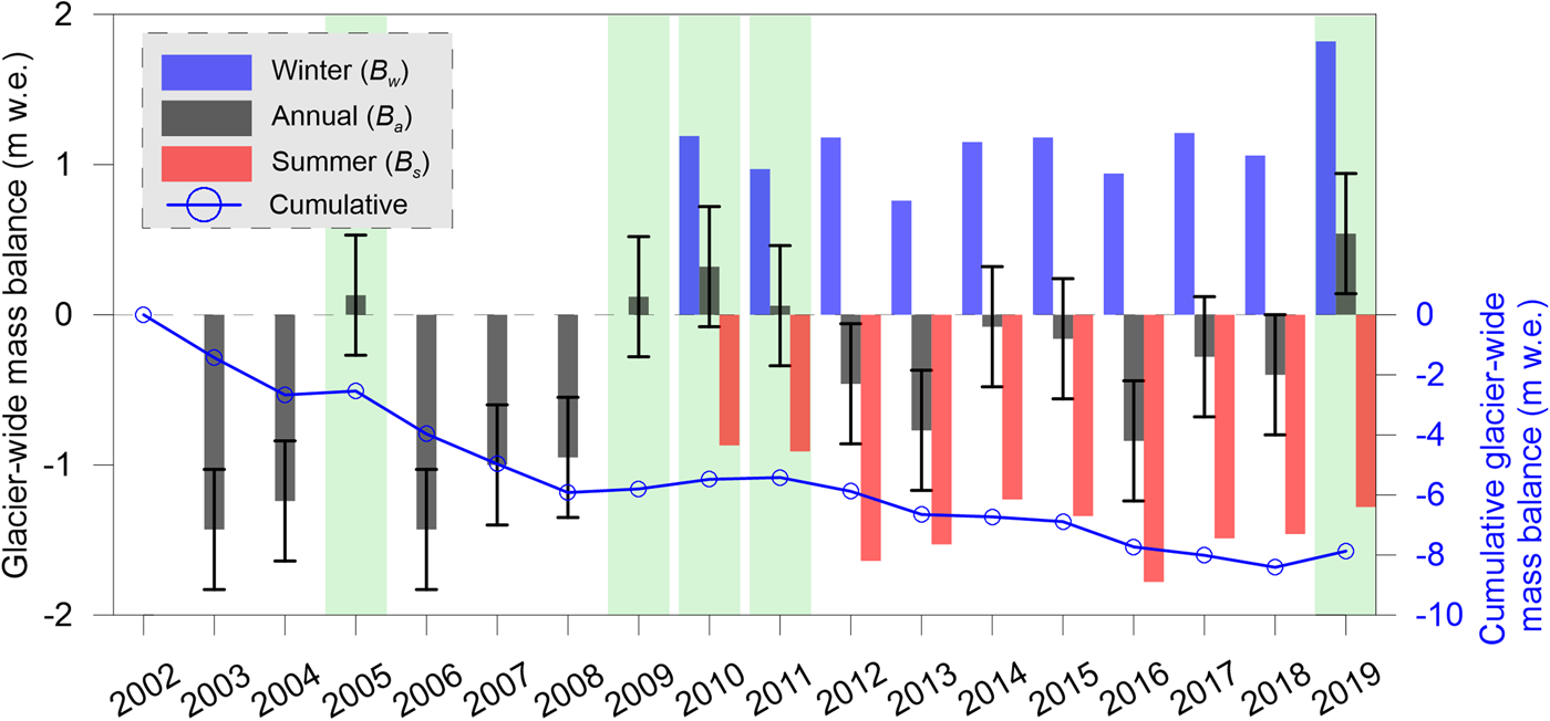
Fig. 4. Glacier-wide (histograms) and cumulative (blue circles) mass balance of Chhota Shigri Glacier between 2002 and 2019. Blue, black and red represent winter, annual and summer glacier-wide mass balance. Green shades are the years with positive B a. B a (2002/03–2013/14) and B w and B s (2009/10–2012/13) are from Azam and others (Reference Azam2016). This study: annual glacier-wide (2014/15–2018/19; 5 years) and seasonal mass balance (2013/14–2018/19; 6 years).
4.4 Sub-seasonal ablation rate
Maximum ablation was observed in late July (~−5 to −8 cm w.e. d−1 in the clean ice area), while minimum ablation was observed in late September (~−2 to −4 cm w.e. d−1) for the period 2015–2019. Mean ablation rates on the debris-covered part were found to be −2.9, −2.6 and −1.8 cm w.e. d−1 in July, August and September corresponding to a mean of −2.4 cm w.e. d−1. Ablation rates were approximately twice as high on the clean ice surface −5.1, −4.8 and −2.6 cm w.e. d−1 in July, August and September, corresponding to a mean of −4.2 cm w.e. d−1 (Table 3). The higher surface melt is associated with the higher incoming short-wave radiation and air temperature over the clean ice region in July, August and September (Fig. 2). The daily melt rate was lower during positive mass-balance years, e.g. 2019 (−3.7 cm w.e. d−1 for clean ice) compared to high negative mass-balance years, e.g. 2016 (−4.3 cm w.e. d−1 for clean ice) and 2018 (−4.3 cm w.e. d−1 for clean ice). A quadratic polynomial function was fitted on all the point ablation data from different years to understand the altitude dependency of ablation on the glacier following standard glaciological practice (Kaser and others, Reference Kaser, Fountain and Jansson2003; Shah and others, Reference Shah, Banerjee, Nainwal and Shankar2019). The polynomial function analysis provides a better description of the mass-balance variation and altitude/debris cover dependency (Figs S4–S8). The ablation rates for any given period (when relatively large measurement points are available) have a larger scatter below 4400 m a.s.l. due to the heterogeneous debris cover, whereas the points are less scattered between 4700 and 4800 m a.s.l. due to a similar ablation pattern. The polynomial fitted plots for all the measured years given in Figures S4–S8 conform to this general pattern. The daily melt rates calculated for Chhota Shigri (Table 3) correspond well to the melt rates of the Sutri Dhaka Glacier (located in the same catchment only ~15 km apart), ranging from −2.6 to −4.6 cm w.e. d−1 between August and September 2013 (Sharma and others, Reference Sharma2016), but are slightly lower to that of Batal Glacier (close to Sutri Dhaka) ranging from −2.3 to −5.8 cm w.e. d−1.
Table 3. Summary of sub-seasonal ablation measurements from the Chhota Shigri Glacier between 2015 and 2019

The total observation period for each of the years is given in Julian days. June and October datasets are not shown being too short to compute the monthly average.
4.5 Cumulative point mass balance since 2002
Four ablation and one accumulation sites were selected for computing the cumulative point mass balance based on the availability of uninterrupted measurements. Figure 5 shows the cumulative point mass balance measured at different glacier surfaces (debris, clean ice and snow/firn) and altitudes on the Chhota Shigri Glacier between October 2002 and September 2019 (17 years). Glacier surface conditions as well as mean and cumulative point mass balances are provided in Table 4. Note that the altitudes of point locations varied (±20 to 30 m) in different years because (i) stakes could not be installed exactly on same locations and (ii) glacier surface altitude changes at the same locations.
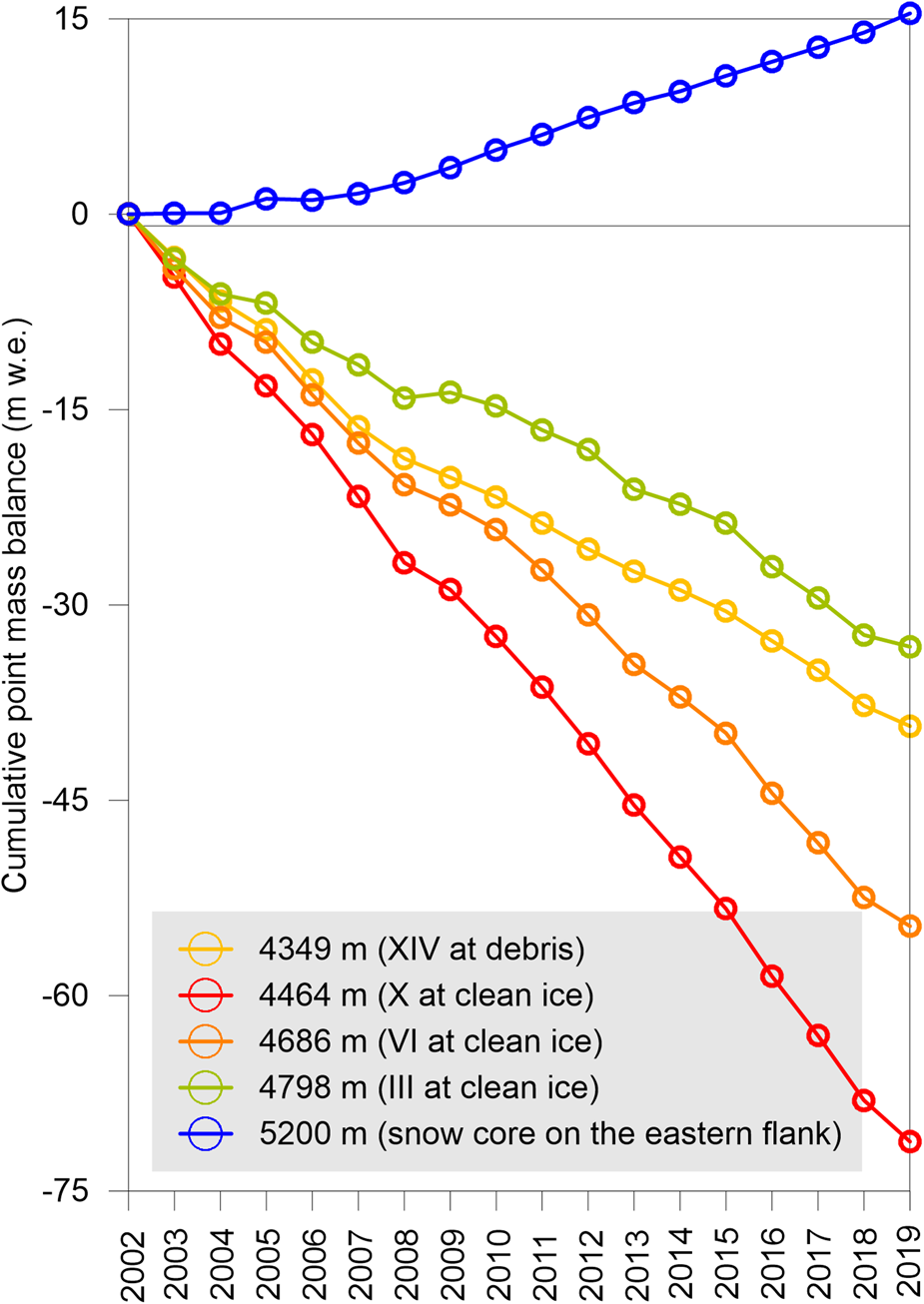
Fig. 5. Cumulative point mass balance measured at four ablation and one accumulation sites on Chhota Shigri Glacier between 2002 and 2019. The legend gives the altitude and surface type of the stakes/core. A year represents the hydrological year, e.g. the point mass balance of 2003 represented the hydrological year 2002/2003. Measurement dates are given in Table S3. Gaps and calculation details are provided in the legend of Table 4.
Table 4. Cumulative point mass balance recorded at different locations representing three different surfaces (debris, clean ice and snow/firn) between October 2002 and September 2019 (17 years)

In the absence of accumulation measurements at 5200 m a.s.l. for a few years, measurements at 5180/5190 m a.s.l. were taken. From 2008/09 onward, the accumulation values at Core A (5200 m a.s.l.) are the mean of 2–4 individual core measurements between 5150 and 5200 m a.s.l. except for 2017/18 where extrapolated values were used (see Section 3.2.1).
On the debris-covered surface, the mass balance was significantly less negative compared to the clean ice areas with a cumulative value of −39.31 m w.e. at 4349 m a.s.l. for the period 2002–2019 corresponding to a mean of −2.18 m w.e. a−1 (Table 4). The most noticeable cumulative melting recorded on the clean ice area was found to be −71.21 m w.e. at 4464 m a.s.l. corresponding to a mean of −3.96 m w.e. a−1, followed by −54.67 m w.e. at 4490 m a.s.l. corresponding to a mean of −3.04 m w.e. a−1. The cumulative point mass balance at 4798 m a.s.l. was found to be −33.21 m w.e. corresponding to a mean of −1.84 m w.e. a−1, the significantly lower values being attributed to its higher altitude, which is ~250 m lower than the mean equilibrium line altitude (ELA) of the glacier. The cumulative point accumulation at 5200 m a.s.l. was found to be +15.42 m w.e. corresponding to a mean of +0.91 m w.e. a−1. Accumulation measurements at 5200 m a.s.l. are almost similar over the 17 years except in the early years, i.e. 2003, 2004 and 2006 when it was significantly lower (0.07, 0.02 and −0.10 m w.e.).
4.6 Annual and cumulative glacier-wide mass balance, ELA and AAR
Here, we present the new dataset of B a for the period 2014/15–2018/19 (Table 2). Figure 4 shows B a, B w, B s and cumulative mass balance since 2002. Inter-annual variability of B a was moderate (SD of ±0.62 m w.e. a−1) with five positively balanced years during 2002–2019. The mean B a of the Chhota Shigri Glacier was −0.46 m w.e. a−1 for the period 2002–2019, which is close to the Himalayan mean value of −0.59 m w.e. a−1 for the period 1975–2015 (Azam and others, Reference Azam2018) as well as global average value of −0.48 ± 0.20 m w.e. a−1 for the period 2006–2016 (Zemp and others, Reference Zemp2019). The cumulative B a was −7.87 m w.e. during the last 17 years.
ELA and accumulation area ratio (AAR) for the studied years are reported in Table 2. ELA for 2014/15–2018/19 was calculated using the regression line (lines in Fig. 3a) extracted through the annual point mass balance of the main glacier body (excluding debris-covered area) between 4400 and 5200 m a.s.l. ELA of the corresponding year was used to distinguish the ablation and accumulation areas for calculating AAR. Overall since 2002, ELA varied from a minimum of 4905 m a.s.l. in 2004/05 (B a: +0.13 m w.e.) to a maximum of 5235 m a.s.l. in 2002/03 (B a: −1.43 m w.e.). ELA and AAR showed a strong correlation with B a (R 2 = 0.88 and 0.91) (Fig. S9). ELA for a zero B a (steady-state; ELA0) was also derived from the regression between B a and ELA over 2002–2019, which is ~4974 m a.s.l. Similarly, AAR value for a zero B a (AAR0) was derived as ~60% for zero B a (Fig. S9).
4.7 Annual surface velocities
Ice velocity at Chhota Shigri Glacier was first measured in 2003 (Wagnon and others, Reference Wagnon2007). For the present study, annual surface ice velocity measurements were performed between 2009 and 2017. However, some data gaps exist due to discontinuous DGPS signals, loss of stakes, as well as risky accessibility in a few years. All the measurements were performed along the flow lines of the eastern (Fig. 6a) and western flank (Fig. 6b).

Fig. 6. Surface ice velocities plotted as a function of distance from the snout in the eastern flank (main glacier body) (a) and western flank (b). Lower ablation zone (LAZ; <4400 m a.s.l.), middle ablation zone (MAZ; 4400–4600 m a.s.l.) and upper ablation zone (UAZ; 4600–4950 m a.s.l.) are shown in the eastern flank panel.
In the eastern flank, ice velocities range from 6 to 45 m a−1 and vary with altitude. In the LAZ (<4400 m a.s.l.) where debris exists, glacier moves slowly with a rate of 13, 12, 8 and 15 m a−1 in 2010, 2011, 2012 and 2013, respectively. Ice velocity is even slower with ~6–7 m a−1 at ~4300 m a.s.l. where glacier surface is completely covered by debris with varying size and thickness. In the middle ablation zone (MAZ; 4400–4600 m a.s.l.) where clean ice is exposed, the glacier moves considerably faster than LAZ with a rate of 29, 29, 26 and 22 m a−1 in 2010, 2011, 2013 and 2016, respectively. In the MAZ, ice movement is maximum between 4500 and 4600 m a.s.l. (~35 m a−1 in 2010 and ~33 m a−1 2011). Glacier ice flow is the highest in the upper ablation zone (UAZ; 4600–4950 m a.s.l.) where the glacier is at its widest and crevassed (4650–4700 m a.s.l.) with steep surface slope. In the UAZ between 4800 and 4830 m a.s.l., the fastest movement of ice with a rate of 45, 44 and 44 m a−1 was measured in 2010, 2012 and 2013, respectively. We observe two peaks in surface velocity, at ~3 and ~6 km from the snout (4600 and 4850 m a.s.l.) which is consistent with the maximum ice thickness observed from ground-penetrating radar (Azam and others, Reference Azam2012).
In the western flank, the glacier moves slightly slower than eastern flank (Fig. 6b). There is likely to be a limited sensitivity of glacier velocity to changes in annual mass balance as previously noted for 2003–2006 (Wagnon and others, Reference Wagnon2007). In the UAZ, the surface ice flows with a rate of 28, 31, 29, 29, 29, 28 and 30 m a−1 in 2010, 2011, 2012, 2013, 2013/15, 2016 and 2017, respectively. Fastest movement of ice with a rate of >30 m a−1 was recorded at ~4800 m a.s.l. at the confluence of the western and eastern flank (Fig. 1).
4.8 Daily and monthly discharge
Meltwater from Chhota Shigri Glacier drains through a combination of numerous supraglacial streams, moulins and subglacial channels as observed during the fieldwork. Half hourly values of water level were used to compute daily mean discharge. Over the entire ablation season (May–October) between 2010 and 2016, daily mean discharge varied from 0.3 to 17.4 m3 s−1 corresponding to a mean of 6.2 m3 s−1 (Table 5). The mean summer discharge was the lowest in 2011 at 3.5 m3 s−1 and the highest in 2013 at 9.6 m3 s−1.
Table 5. Monthly mean discharge at Chhota Shigri Glacier stream between 2010 and 2016

Annual means are the average of all available datasets in a particular year.
Mean monthly discharge for June, July, August and September was observed to be 5.5, 8.9, 7.5 and 3.7 m3 s−1 between 2010 and 2016 (Fig. 7a). Only July, August and September had the full-month record of discharge for all the studied years (Table 5). Analysis of this monthly discharge indicates maximum discharge in July (43%) followed by August (38%) and September (19%) (Fig. 7c). As such, July and August receive more than 80% of the total annual discharge, corresponding to the warmest months in the summer (Fig. 7b).

Fig. 7. (a) Mean monthly distribution of discharge, (b) mean monthly air temperature at the AWS-M (4863 m a.s.l.), and (c) monthly discharge percentage (%) of the Chhota Shigri Glacier stream during 2010–2016.
5. Discussions
5.1 Local meteorology and mass balance
To understand the climatic influences on glacier mass balance, we compared annual and seasonal T air records from the AWS-M (4863 m a.s.l.) and P from the Geonor gauge (3850 m a.s.l.), respectively, with mass-balance data (Fig. 8). To maintain consistency in all analysis, B a, B w and B s were compared with annual, winter (DJFM) and summer (JJAS) T air and P.
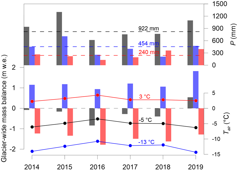
Fig. 8. Annual, winter and summer mass balances are shown by, respectively, black, blue and red histograms. The annual, winter, summer precipitations and air temperatures are shown by black, blue, red histograms and dots, respectively. The mean air temperature is from AWS-M while the precipitation sums are from Geonor gauge except for 2013/14 hydrological year where precipitation was obtained from the IMD-gridded dataset (0.25° × 0.25°; closest grid). Dashed lines are the mean precipitation (2012–2019) of annual, winter (DJFM) and summer (JJAS), respectively. Air temperature values are the mean (2009–2019) of annual, winter and summer, respectively.
The B a was negative for negative P anomaly years, e.g. 2015/16, 2016/17 and 2017/18 and positive with positive P anomaly year, e.g. 2018/19 (Fig. 8). B w and winter P were also related: higher B w years with positive P winter anomalies, e.g. 2014/15 and 2018/19, and lower B w with negative P winter anomalies, e.g. 2015/16 and 2017/18. Also B s showed a good agreement with summer P. B s were comparatively less negative in 2013/14 and 2018/19 (−1.23 and −1.28 m w.e.) with higher summer P except in 2017/18 (−1.62 m w.e.), whereas B s were more negative in 2014/15, 2015/16 and 2016/17 (−1.34, −1.78 and −1.49 m w.e.) with lower summer P.
T air was +1.93°C above the long-term mean in 2015/16 which resulted in a highly negative B a of −0.84 m w.e., whereas T air was −0.72 and −0.92°C below the long-term mean in 2013/14 and 2018/19, corresponding to a nearly balanced and positive B a of −0.08 and 0.54 m w.e. B w and B s values also showed a consistent relationship with winter and summer T air (Fig. 8).
Even though the mean summer T air at AWS-M during the study period was positive (Table S1), daily mean T air occasionally dropped below the freezing point (Fig. 9), suggesting that precipitation could fall as snow. This was probably the prevailing case in 2013/14 and 2018/19 when B a were close to zero and positive (with positive P anomaly) compared to the other years. These snowfalls increased the surface albedo of the glacier during the high melting period in summer between August and September (Figs 9a, c), thus reducing the melting, resulting in less negative B s in 2013/14 and 2018/19 (Fig. 8). In comparison, a significant snowfall event was recorded in late September 2017/18 (169 mm w.e. of snowfall recorded during 22–24 September 2018 by Geonor; Fig. 9b), but B a was still highly negative. Probably, the snowfalls were not in time to protect the glacier from higher melting. This year thus was characterized by highly negative B s (Fig. 8), indicating the importance of timing of summer-monsoon snowfall events, as late-September is already a low-melt period due to lower temperatures and does not have much control over B a. This explicit analysis is consistent with the fact that B a is dependent on the summer-time local meteorology and precipitation frequency/amount, which is also consistent with the results of our earlier surface energy-balance study (Azam and others, Reference Azam2014a). Such a pattern of mass balance was noted earlier in Nepal (Fujita and Ageta, Reference Fujita and Ageta2000) and Tibetan Plateau (Mölg and others, Reference Mölg, Maussion, Yang and Scherer2012; Zhang and others, Reference Zhang2013).

Fig. 9. Comparison of daily summer (1 June to 30 September) air temperature (black), albedo (red) and precipitation (blue) for 2013/14 (a), 2017/18 (b) and 2018/19 (c). Air temperature and albedo recorded at the AWS-M. Precipitation was recorded at the base camp in Geonor gauge during 2013/14 and 2017/18 while manual rain gauge was data used in 2018/19. B a of the corresponding years is also shown on top of the respective panel. Precipitation data gaps (green line) are from 1 June to 17 July and 12 to 24 August in 2013/14, 25 to 30 September in 2017/18 and 1 to 24 June in 2018/19.
The correlation matrices between annual and seasonal mass balance and meteorological variables were used to support linkages between meteorological conditions and mass balance (Table S4). B a is positively correlated on an annual scale with RH (R 2 = 0.68), P (R 2 = 0.67) and u (R 2 = 0.63). In summer, when the atmosphere is relatively warm (2.8°C; mean of 2012–2019) and T air is always above the freezing point (∑T air+ = 378.3°C; mean of 2012–2019), B a is negatively correlated with the T air (R 2 = −0.75) and ∑T air+ (R 2 = −0.70). This means that higher T air implies high negative mass balance, and vice versa. L in and S in showed a highly positive correlation with T air, especially during the pre-monsoon (R 2 = 0.85 for L in vs T air and R 2 = 0.86 for S in vs T air) and summer (R 2 = 0.91 for L in vs T air and R 2 = 0.78 for S in vs T air). This could have an impact on the mass balance. A mean L in of 235 and 282 W m−2 in the pre-monsoon and summer, respectively, which are much higher than the other seasons, resulting in higher melting due to high long-wave emissions from the ice-free areas. In the following, we analyse the relationship between the B a and seasonal (winter and summer) climate variables. During summer, B a and P showed a highly positive correlation (R 2 = 0.73), but surprisingly the correlation with RH was not significantly positive (R 2 = 0.05). Although post-monsoon precipitation is negligible (19 mm month−1), the correlation coefficient is higher (R 2 = 0.25) than that of pre-monsoon (R 2 = 0.01) when precipitation was ~5-times higher (100 mm month−1). In winter, B a was relatively well correlated to P (R 2 = 0.51), coupled with a highly positive correlation with RH (R 2 = 0.86). This relationship is likely due to the moisture content of WDs during winter resulting in high P (~49% of annual precipitation) on the Chhota Shigri Glacier.
Thus B a of the Chhota Shigri Glacier is mainly controlled by T air with a sub-equal influence of summer snowfall, as suggested by previous studies (Azam and others, Reference Azam2014a, Reference Azam2014b). Such a relationship between B a and the meteorological variables is not very clear in the glaciers of the Everest region; yet Wagnon and others (Reference Wagnon2013) and Sherpa and others (Reference Sherpa2017) noted a weak link between glacier mass loss and monsoon precipitation deficit. Moreover, in Chhota Shigri Glacier catchment, the mean annual T air is lower at −5.4°C (Table S1) than in the Everest region where the mean annual T air remains at −3.9°C (2010–2015; at 5360 m a.s.l.; Sherpa and others, Reference Sherpa2017).
5.2 Comparison of mass balance over the Lahaul-Spiti region
We compiled all available mass-balance records on Chhota Shigri Glacier and for the entire Lahaul-Spiti region from glaciological and geodetic approaches (Fig. S10). The geodetic mass balance of the Chhota Shigri Glacier was estimated to be −0.23 ± 0.28 and −0.27 ± 0.13 m w.e. a−1 using SPOT5-Pléiades and ASTER stereo imageries, respectively, over 2005–2014 (Brun and others, Reference Brun, Berthier, Wagnon, Kääb and Treichler2017). These estimates are relatively lower than the glaciological mass balance of −0.41 ± 0.40 m w.e. a−1 for the same period. Vijay and Braun (Reference Vijay and Braun2016) reported a geodetic mass balance of −0.89 ± 1.13 m w.e. in 2012/13 for Chhota Shigri Glacier using TanDEM-X data, which fits well with the glaciological B a of −0.77 ± 0.40 m w.e for 2012/13 (Azam and others, Reference Azam2016). Geodetic mass-balance estimate of −0.40 ± 0.20 m w.e. a−1 over 2000–2016 for the Lahaul-Spiti region (705 glaciers covering 4477 km2 area) using ASTER dataset (Brun and others, Reference Brun, Berthier, Wagnon, Kääb and Treichler2017) also agrees fairly well with the glaciological long-term mean B a of −0.55 m w.e. a−1 for Chhota Shigri Glacier over the period 2002–2016. Compiling all the existing short-term in situ mass-balance measurements and the geodetic results, Bolch (Reference Bolch2019) reported a mass loss of −0.50 m w.e. a−1 over ~2000–2015 for the western Himalaya (including Lahaul-Spiti). Hence, both glaciological and geodetic techniques reveal a moderate and similar mass loss for Chhota Shigri and Lahaul-Spiti glaciers during the past two decades, also highlighting the representativeness of Chhota Shigri as a benchmark glacier for the entire Lahaul-Spiti region as proposed earlier by Vincent and others (Reference Vincent2013).
5.3 Dynamic behaviour and adjustment
Surface ice velocity is normally driven by the mass budget of the glacier (Cuffey and Paterson, Reference Cuffey and Paterson2010). A negative (positive) mass balance will result in decreased (increased) ice flux through changes in glacier ice thickness and velocity. An extensive field measurement campaign was carried out on the Chhota Shigri Glacier which provides one of the best and longest dataset (Section 4.7 and Fig. 6) to understand the dynamic behaviour of glaciers in the western Himalayan region. The mean B a was negative at −0.46 m w.e. a−1 between 2002 and 2019; therefore, changes in ice flow and thickness are expected. In this section, we compare the measured surface ice velocities of 2010/11 and 2015/16 with the velocities of 2003/04.
Even though measurements have not been carried out at exactly the same locations, the reduced surface velocities in both eastern and western flanks were found since 2003/04 (Fig. 6 and Table 6). In the eastern flank, the velocities are reduced by 25% in 2010/11 and 42% in 2015/16 compared to 2003/04 velocities; however, at higher altitudes, 4800 m a.s.l. and above, the velocity changes were significantly less (16–17%; Table 6). These reduced velocities, particularly in the MAZ, are in line with the thinning of ~8 m observed on Chhota Shigri Glacier over 1988–2010 (Vincent and others, Reference Vincent2013). Further, another study also reported the thinning of ~13 m below 4600 m a.s.l. over a recent period of 2002–2014 using Terra ASTER dataset (Garg and others, Reference Garg, Shukla, Tiwari and Jasrotia2017). At the regional scale, Dehecq and others (Reference Dehecq2019) reported a reducing velocity of ~34% per decade for the period 2000–2017 in the Lahaul-Spiti region using Landsat-7 imageries, which is in broad agreement with our result of 25% velocity reduction during 2003/04–2010/11 and 42% during 2003/04–2015/16.
Table 6. Comparison of surface ice velocities of 2010/11 and 2015/16 with 2003/04 on the eastern flank of Chhota Shigri Glacier

Velocities of 2003/04 are obtained from Wagnon and others (Reference Wagnon2007). Stakes were re-installed (when melted out) ~30 m above the initial location in view of the observed ice velocity.
5.4 Meteorological factors, statistical relationships and time-lag of discharge
Figure 10 shows the daily catchment meteorology recorded at AWS-M and the discharge measured near Chhota Shigri Glacier catchment outlet for the period 2010–2016. Discharge from the Chhota Shigri catchment closely follows T air variation. Figure S11 (a close view of the precipitation-albedo effect on discharge) shows that in 2010 (7–8 July) and 2011 (~11 August), fresh snowfall (evident from near-zero T air) indicated by a sudden increase in surface albedo was accompanied by an immediate reduction in discharge and an increase in time-lag. However, this relationship may vary depending on the occurrence of precipitation type at different sites. At the AWS-M site, located at ~1000 m higher altitude than the discharge site, due to low temperature, precipitation may fall as snow, resulting in an increase in albedo, hence decrease in melting. However, the same precipitation may fall as rain at lower altitudes due to comparatively higher T air during the summer. In such a case, proglacial discharge could increase due to the addition of rainfall from the lower parts of the catchment.

Fig. 10. Daily means of T air, discharge, P, albedo, RH, u, S in and L in at AWS-M. T air, albedo, RH, u and S in are the daily means for the period 1 May 2010–31 October 2016, whereas L in is the daily means between 23 May 2010 and 21 February 2015. The daily P between 12 July 2012 and 31 October 2016 were collected by Geonor. Precipitation of IMD-gridded dataset was used from 1 May 2010 to 11 July 2012 and 8 October 2013 to 17 July 2014 where the gauge was not functional due to the battery failure.
The role of albedo shoot-up by snowfall on the glacier is indicated by the extent to which the discharge is dampened just after snowfall events when the T air was below freezing point. These snowfall events significantly control the discharge, as modulated by T air. Albedo-enhancing snowfall events in September generally resulted in a marked dip in proglacial discharge and marked the end of the ablation season (Fig. 10). Although various meteorological parameters play an important role (e.g. solar radiation), it is T air that best simulates glacier melt (subsequently proglacial discharge) on the Chhota Shigri Glacier.
To determine the statistical relationship of different meteorological variables with discharge, between 2010 and 2016, we obtained the coefficient of determination (R 2) of each meteorological variable with discharge on a daily scale (Fig. 11). The glacial discharge has a good positive correlation with T air (R 2 = 0.66), L in (R 2 = 0.58) and RH (R 2 = 0.39), but a negative correlation with P (R 2 = −0.02) and u (R 2 = −0.28). The generation of discharge is primarily determined by the availability of heat on the glacial surface, therefore the discharge showed a good correlation with T air. The daily variation of T air seems to be correlated with cloudiness that is more when L in is higher, which positively influences the discharge (Fig. 11). Given the higher T air during the summer period, the glacier surface remains at 0°C even during nights (Azam and others, Reference Azam2014a) and L in emitted by the surrounding valley walls probably governs the glacier melt and consequent discharge in the night. Chhota Shigri Glacier receives ~29% of annual P in summer (mostly as snowfalls on the glacier). However, summer monsoon snowfalls were found to reduce the melt on Chhota Shigri Glacier, but the snowfalls on the non-glacierized area (53% of total catchment at the discharge site) provide additional water at the discharge site and therefore makes the precipitation–discharge relationship quite complicated (Azam and others, Reference Azam2019; Kumar and others, Reference Kumar2020).

Fig. 11. Correlation matrix of various daily meteorological variables recorded at the AWS-M with discharge measured at the discharge site in the Chhota Shigri Glacier catchment for the period 2010–2016. Cross marks denote the insignificant correlation at a significant level of p < 0.05.
There is a time-lag between meltwater generation over the glacier and its emergence at the discharge site. In general, the time-lag depends on the distance; water has to travel through and beneath the glacier (Benn and Evans, Reference Benn and Evans1998; Pottakkal and others, Reference Pottakkal2014). Here, we attempt to quantify the time-lag using the half-hourly dataset of discharge and T air. Due to the half-hourly discharge data availability in 2012, different periods were considered to understand the variations of discharge delaying characteristics. We picked clear-sky days in our analysis, with no/minimum rain over the glacier. Figure 12 shows the discharge and T air variation during the early melting (June), peak melting (July and August) and late melting (September) periods.

Fig. 12. Diurnal variation of discharge (blue) and T air (red) for selected clear weather days (zero precipitation) during early melt (June), peak melt (July and August) and late melt (September) periods over the ablation season of 2012.
We do not observe any prominent discharge maxima despite the high-temperature peaks in the early melt (June) and late melt (September) seasons (Figs 12a, d). This is most probably due to the high snow thickness (Singh and others, Reference Singh, Kumar and Kishore2011) and the resultant high surface albedo that allows minimal absorption of incoming solar radiation during early melt season and the low solar inclination during the late melt season. The refreezing of the meltwater into the snowpack could be another possible explanation for no prominent discharge maxima in the early and late melt seasons. The discharge was the highest at ~8–13 m3 s−1 with a pronounced diurnal cycle in July–August (Figs 12b, c). Discharge closely follows T air with ~2–4 h of time-lag.
The time-lag between T air at AWS and discharge at discharge site includes melting of snow/ice, as well as the travel time by meltwater through supra-glacial and sub-glacial channels. To understand the travel time in the sub-glacial system, we performed two dye tracer experiments in two different moulins in August 2016 (Table 7). Moulin-1 (M-1) is located in the MAZ, while the moulin-2 (M-2) in the LAZ. Figure 13a shows the dye concentration curve from the injections into M-1 and M-2, respectively, measured at the discharge site. The pulses were distinguished by a distinct peak with a steep rising limb and a more or less gentle and long-tailed falling limb. The time taken by the dye cloud to reach the discharge station was 52 and 18 min, respectively, from M-1 and M-2 (Fig. 13). Though moulins M-1 and M-2 are only ~1.5 km away from each other, we note a difference in arrival time of ~34 min between M-1 and M-2. This long travel time between M-1 and M-2 could be due to crevasse or some complicated drainage network between M-1 and M-2. We also observed small multiple curves from M-2 which could be linked to a small storage system within the glacier drainage system. Although our results are preliminary, we need more such experiments for the future to arrive at a clear statement about the sub-glacial network and its impact on discharge.

Fig. 13. (a) Dye concentration curve resulting from injections at M-1 and M-2 in the Chhota Shigri Glacier, and (b) location of the moulins and dye measurement site.
Table 7. Attributes of Moulin 1 and 2 for the dye tracer experiment performed on 14 August 2016

6. Conclusion
The B a of Chhota Shigri Glacier was measured using the glaciological method for the period 2002–2019 and found to be negative with a mean of −0.46 ± 0.40 m w.e. a−1, corresponding to a cumulative wastage of −7.87 m w.e. over the last 17 years. The mean winter mass balance was 1.15 m w.e. a−1, while mean summer mass balance was −1.35 m w.e. a−1 over 2009–2019. The debris cover greatly protects the lowest part of the glacier from melting through providing a shield. More than 600 sub-seasonal ablation measurements during June and September over 2015–2019 suggest that the maximum ablation of ~−5 to −8 cm w.e. d−1 (in the clean ice area) occurs in late July, while the minimum of ~−2 to −4 cm w.e. d−1 in late September and early October. The cumulative point mass balance over the last 17 years shows that the mass lost in the LAZ (~−70 m w.e.) is significantly higher than the cumulative point accumulation (+15 m w.e.) in the accumulation zone. An analysis of the seasonal and annual mass balances and in situ meteorological variables measured at the AWS-M reveals that the B a is primarily controlled by T air, with a sub-equal influence of summer snowfall in terms of intensity and timing.
We observed a good agreement between the long-term glaciological B a of the Chhota Shigri Glacier and the region-wide estimated geodetic mass balance of the Lahaul-Spiti region, indicating the representativeness of Chhota Shigri as a benchmark glacier for the Lahaul-Spiti region. Highest surface ice velocities were found in the UAZ, while LAZ filled with debris had the slowest velocity. Surface ice velocity of the Chhota Shigri Glacier has slowed down by 25–42% between 2003 and 2016, particularly in the lower and MAZs in response to mass loss, while no substantial change was observed at higher altitudes. The stream discharge in July and August comprises more than 80% of the total discharge of the summer. Discharge is primarily controlled by the air temperature throughout the summer season.
The mass balance of Chhota Shigri Glacier since 2002 is the longest continuous series in the HKH region and should be continued as a benchmark glacier for climate change studies. In addition, we recommend to enhance the glacier monitoring network in this region with continuous glacier-wide mass-balance measurements in combination with local meteorology, ice velocity, stream discharge, etc., to better understand the behaviour of Himalayan glaciers in response to ongoing climate change.
Supplementary material
The supplementary material for this article can be found at https://doi.org/10.1017/jog.2020.42.
Acknowledgements
We thank Jawaharlal Nehru University, New Delhi for providing all the facilities to carry out this work. We thank the field assistant B. Adhikari and the Nepali porters who have taken part in successive field trips, sometimes in harsh conditions. We are also grateful to two anonymous referees and the Scientific Editor Carleen Tijm-Reijmer, whose detailed comments have significantly improved the paper. The funding agencies and project collaborators supported this work: DST-Govt. of India, MoES, SAC-ISRO, IFCPAR/CEFIPRA, INDICE, GLACINDIA and CHARIS. AM is grateful to UGC-RGNF, and DAAD Bi-nationally Supervised PhD Fellowship (Germany) for providing financial support for his PhD. MFA acknowledges the research grant from INSPIRE Faculty award (IFA-14-EAS-22). We thank Patrick Wagnon and Christian Vincent for their contribution in fieldwork and Pierre Chevallier for his contribution to discharge measurement. We acknowledge the IMD for sharing the dataset.
Author contributions
AM, ALR, TA and MFA conceptualized the study. ALR supervised the study. AM performed the analysis, developed the figures and wrote the paper. All authors contributed significantly in fieldwork and to improve the draft manuscript and supported the data analysis.


 Open access