2.1. Governing equations

The present approach comprises a RANS computation of the full boundary layer domain used as a precursor calculation and a smaller LES domain situated within. This allows for the scale resolving LES to be used where it is required in predicting the interaction between the multiple vortices and the turbulent boundary layer, with the inlet conditions supplied from the precursor RANS calculation and a vortex model. Figure 2 shows the set-up of the two domains.

Figure 2. Diagram showing the set-up of the RANS domain and LES domain for the base case of a ZPG turbulent boundary layer.

In the LES region, the filtered Navier–Stokes equations are solved. These are given by

(2.1)\begin{equation} \frac{\partial \langle \boldsymbol{u}_i\rangle}{\partial \boldsymbol{x}_i} = 0,\quad \frac{\partial \langle \boldsymbol{u}_i\rangle}{\partial t} + \frac{\partial \langle \boldsymbol{u}_i \boldsymbol{u}_j\rangle}{\partial \boldsymbol{x}_j} ={-}\frac{1}{\rho}\,\frac{ \partial \langle p\rangle }{ \partial \boldsymbol{x}_i } + \nu\,\frac{ \partial^2 \langle \boldsymbol{u}_i\rangle }{ \partial \boldsymbol{x}^2_j }, \end{equation}

where the vector ${\boldsymbol{x}}_i$ comprises ${x}_1 = {x}$, ${x}_2 = {y}$ and ${x}_3 = z$, being the streamwise, wall-normal and spanwise directions, respectively. Correspondingly, ${\boldsymbol{u}}_i = ({u}, {v}, {w})$ is the velocity vector field, with the subscript $i$ denoting the direction. Also, $p$ is the pressure field, $\rho$ is the fluid density, and $\nu$ is the kinematic viscosity of the fluid. The angle brackets denote a filtering operation, and the turbulence stress terms $\langle \boldsymbol{u}_i \boldsymbol{u}_j\rangle$ comprise both the resolved term and the effect of the sub-grid scales, which are modelled using a sub-grid scale (SGS) model. When presenting results, an overbar represents time averaging, and a dash represents the remaining fluctuating part of the field.

In order to relax the grid requirements needed to complete wall-resolved LES (WRLES), a hybrid RANS-LES model was used. By using the improved delayed detached eddy simulation (IDDES) implementation of Shur et al. (Reference Shur, Spalart, Strelets and Travin2008) in the configuration designed for wall-modelled LES (WMLES), the grid spacing in the streamwise and spanwise directions can be increased considerably, since only the outer region of the turbulent boundary layer, $y/\delta >0.1$, is treated with LES, while the inner region is handled with a RANS model. To appreciate the magnitude of this saving, Piomelli (Reference Piomelli2008) estimated that for $Re\approx 10^6$, the number of mesh cells required to resolve the inner region of the boundary layer, as required in WRLES, is around two orders of magnitude higher than the number of cells needed in the outer region. In this study, the Spalart–Allmaras one-equation RANS model is used to model turbulence quantities in the inner boundary layer, before switching rapidly to full LES away from the wall. The WMLES branch is designed to be activated in the presence of unsteady inflow conditions provided that the grid is sufficiently fine for resolving the dominant eddies found within a turbulent boundary layer. More details of the WMLES model can be found in Appendix A and in the paper of Shur et al. (Reference Shur, Spalart, Strelets and Travin2008).

The inlet boundary conditions to the LES domain are obtained from the RANS domain, for which the Spalart–Allmaras turbulence model is used, details of which can be found in the paper of Spalart & Allmaras (Reference Spalart and Allmaras1992). The current work uses a formulation without the trip term or ft2 term implemented, and with a limiter on the modified vorticity term to prevent negative values. The Spalart–Allmaras turbulence model was chosen for the background RANS calculation as it is particularly well calibrated for use on boundary layer flows and follows the methodology applied in earlier studies using similar techniques on turbulent boundary layers (Mockett, Haase & Schwamborn Reference Mockett, Haase and Schwamborn2017). In order to transition effectively from the RANS-modelled description of the flow in the precursor calculation to the region of LES, turbulence fluctuations in the velocity field must be introduced as these are not present in the averaged flow field of the RANS calculation. The synthetic eddy method (SEM), first proposed by Jarrin et al. (Reference Jarrin, Benhamadouche, Laurence and Prosser2006), is an efficient method used to introduce fluctuations to the velocity field at the LES inlet that can be applied to inhomogeneous fields. The method superimposes a prescribed number of randomly positioned eddies onto the mean velocity field, which are then scaled to match the spatial estimate of turbulence provided from the RANS model. The resulting fluctuating velocity field contains turbulent structures that are coherent in both time and space, and exist over a range of scales. Further details of the method used in this investigation, including improvements to the original SEM, are presented in the work by Skillen, Revell & Craft (Reference Skillen, Revell and Craft2016).

In this study, the finite volume code OpenFOAM-v1812 is used (Weller et al. Reference Weller, Tabor, Jasak and Fureby1999). For the LES, the coupled momentum and pressure equations are solved using the PISO algorithm with the time integration performed using a second-order backwards differencing, and spatial discretisation done using second-order schemes. For the precursor RANS calculation, the SIMPLE algorithm is used for the coupling of the momentum and pressure equations, with spatial discretisation performed using second-order schemes.

2.2. Boundary conditions

For the precursor two-dimensional RANS calculation, the domain is set up following the validation case of Rumsey, Smith & Huang (Reference Rumsey, Smith and Huang2009). The velocity inlet boundary condition is defined by a uniform Dirichlet condition $U_x = U_0 = 70\,{\rm m}\,{\rm s}^{-1}$. The outlet and top velocity boundary conditions are zero-gradient Neumann conditions, while the lower boundary has an initial section of a symmetrical boundary condition followed by a no-slip wall, as shown in figure 2. The pressure inlet condition is zero-gradient Neumann, with the other pressure boundaries zero-value Dirichlet conditions. The turbulence quantity for the Spalart–Allmaras model at the inflow is set to be three times the kinematic viscosity, $\tilde {\nu } = 3\nu$, based on the recommendation by Spalart & Rumsey (Reference Spalart and Rumsey2007).

For the LES domain, the SEM is used to define the inlet velocity, based on the information from the precursor RANS calculation. The turbulence quantities at the inflow are taken from the value of $\tilde {\nu }$ from the precursor RANS model multiplied by the blending functions $f_B$ and $f_{e1}$ given in Appendix A as (A2a,b) and (A4a,b). A no-slip condition is applied along the lower wall, whilst the outlet and top velocity boundary conditions are zero-gradient Neumann conditions, and the front and back boundaries are periodic in the lateral direction as vortex generators are often found in arrays and match the set-up used by Liu et al. (Reference Liu, Piomelli and Spalart1996). The pressure inlet condition is zero-gradient Neumann with the top, wall and outlet pressure boundaries defined with zero-value Dirichlet conditions.

2.3. Vortices

The vortex generators themselves are not resolved in this study. Instead, a simple vortex model is used to represent their downstream impact on the mean velocity field. The model is then combined with both the RANS turbulent boundary layer profile and the synthetic turbulence fluctuations to provide the inlet condition for the LES domain. In this way, the LES domain can be considered to start immediately downstream of the vortex generator.

A velocity field is generated to model the inclusion of the vortex by using the Batchelor vortex model (Batchelor Reference Batchelor1964). In order to model a vortex pair, two Batchelor vortices are introduced, and in order to enforce the non-permeable condition imposed by the solid wall, two additional mirror vortices are also included beneath the wall, as illustrated in figure 3, corresponding to each of the real vortices. The velocity fields of the individual vortices are created using a form of the Batchelor vortex equations that Velte, Hansen & Okulov (Reference Velte, Hansen and Okulov2009) found matched experimental results. The azimuthal velocity is defined by

(2.2)\begin{equation} V_{\theta} = \frac{q R }{r } \left[ 1-\exp\left( -\frac{r^2}{R^2} \right) \right] , \end{equation}

where $q$ is the strength of the vortex, $r$ is the distance away from the centre of the vortex, and $R$ is a length scale corresponding to the radius of the vortex core. To model the streamwise velocity deficit introduced in real vortex generators by the delta-wing-shaped devices, a velocity component in the streamwise component is included, defined by

(2.3)\begin{equation} V_{x} = q_w \exp \left( -\ln(2)\,\frac{r^2}{R^2} \right) , \end{equation}

where $q_w$ is the strength of the wake, and the constant $\ln (2)$ is used to set the magnitude of $V_x$ at the edge of the core to be half the maximum magnitude. Two vortices and their corresponding mirror vortices can then be defined with centres in the wall-normal direction $y = \pm H_v$, and in the spanwise direction at $z = \pm S_v/2$. In order to enforce the no-slip condition at the wall, the azimuthal velocity is reduced linearly from distance $y/\delta _0 = 0.1$, where $\delta _0$ is the boundary layer height at the LES inlet location. The Batchelor vortex model presented provides an approximation of the vortices found in the wake of a vortex generator and makes the assumption that the vortices are rotationally symmetrical and do not contain a radial component. The effects of these assumptions are considered relatively minor compared to the contribution of the azimuthal velocity component. Only the effect of the vortices on the velocity field is considered here, and no additional turbulence is introduced beyond that from the boundary layer. This limitation of the approach is difficult to avoid as a model of the additional turbulence would depend strongly on the specific geometry of the vortex generators. In § 4.1, the resulting flow of this model is compared to that found experimentally in the wake of a pair of vortex generators by Pauley & Eaton (Reference Pauley and Eaton1988). The comparison suggests that the flow would not be particularly sensitive to additional turbulence contributions, with the interaction between the vortices and the boundary layer turbulence dominating the behaviour.

Figure 3. Diagram showing the set-up of the vortex pair at the inlet to the LES region and the definition of the parameters used in their creation.

The strength ($q$) and radius ($R$) of the vortices can be defined independently in order to achieve a configuration that represents the vortices generated by a skewed vortex generator. As shown in figure 3, when the flow direction is skewed by angle $\alpha$, the relative angles of the vortex generators are $\beta \pm \alpha$, where $\beta$ is the designed angle of the vortex generator. It is then this relative angle that correlates to the strength of each vortex. In this study, the effects of varying vortex configurations are investigated by varying the relative signs of the vortices, with $q_1/q_2 = -1$ describing counter-rotating vortices, and $q_1/q_2 = 1$ co-rotating vortices. The separation distance ($S_v$) between the vortices for both counter-rotating and co-rotating vortex pairs, and the effect of varying the skew angle ($\alpha$), are explored in § 4.3.

2.4. Mesh

The meshes used for the WMLES calculations are constructed according to best practice guidelines from a study of the same baseline case in the EU project ‘Go4Hybrid’ (Mockett et al. Reference Mockett, Haase and Schwamborn2017), and focus on capturing accurately the outer part of the boundary layer at an efficient resolution. The main mesh characteristics for the WMLES cases with and without vortices included are presented alongside those of the RANS mesh in table 1.

Table 1. Properties of the meshes used for both cases.

For the LES calculations, the total number of grid points is $N_{xyz} \approx 7.6 \times 10^6$ for the mesh used for the turbulent boundary layer only. When the vortices are introduced, the domain size is increased in the spanwise direction from $5\delta _0$ to $12.5\delta _0$ in order to capture the vortices as they develop downstream; this specific width is chosen to match the width of the domain used in the reference study by Liu et al. (Reference Liu, Piomelli and Spalart1996). Additional refinement is also included in the $y$-direction to account for the slight increase in boundary layer height, which leads to a larger mesh of size $N_{xyz} \approx 20 \times 10^6$. The wall-normal grid size for the turbulent boundary layer flow and the corresponding blending behaviour is shown to be performing as designed in § 3. The sensitivity to the grid spacing with the inclusion of vortices is shown through the comparison of the vortex development on different grids in § 4.1.

4.1. Validation of method

The central focus in this paper is the vortex generator study reported by Pauley & Eaton (Reference Pauley and Eaton1988), later replicated numerically by Liu et al. (Reference Liu, Piomelli and Spalart1996) using LES with a rescaling method proposed by Spalart & Watmuff (Reference Spalart and Watmuff1993) to rescale the spatially developing boundary layer in a periodic domain. They introduced the vortex pairs using a body force of a similar field as that used in the present work, described in § 2.3. In the current study, the Batchelor vortices are applied at the location corresponding to the first measurement point in the experiment, immediately downstream of the vortex generator. These vortices, henceforth referred to as the primary vortices, were generated with a separation distance $S_v = 11\delta _0/4$, at height above the wall $h_v = 5\delta _0/8$, with radii $R_1 = R_2 = 2.1\delta _0/8$ and the vortex strength in (2.2), $q_1 = -q_2 = 0.37 U_0$. These setting were selected to match the velocity profiles used by Liu et al. (Reference Liu, Piomelli and Spalart1996), as shown in figure 7. These profiles match closely between the current method of applying the vortices to the velocity field of the inlet and the method of applying a body force used by Liu et al. (Reference Liu, Piomelli and Spalart1996). In (2.3), $q_w$ is set as $1.25 |q|$ so that the local minimum streamwise velocity, at the vortex core, is $u = 0.45 U_0$, matching the value in the experiment (Liu et al. Reference Liu, Piomelli and Spalart1996).

Figure 7. The mean velocity components in the $x$-, $y$- and $z$-directions applied at the inlet to the LES domain compared to a Batchelor vortex and the inlet used by Liu et al. (Reference Liu, Piomelli and Spalart1996). The profiles of $U$ and $W$ are located at the vortex core location in the $z$-direction, and the $V$ profiles are shown to each side of the vortex core.

Downstream of the inlet, the development of the peak streamwise vorticity $\omega _x^{max}$, where the vorticity is defined as the curl of the velocity field $\boldsymbol{\omega} _i = \boldsymbol {\nabla } \times \boldsymbol{u}_i$, is shown along the length of the plate in figure 8. This is compared to corresponding values reported in both previous LES and experimental studies. The peak vorticity decay closely matches that reported by Liu et al. (Reference Liu, Piomelli and Spalart1996). In both the present work and the results of Liu et al., the vortex diffuses at a slightly greater rate than the experiment, particularly in the region $x/\delta _0>20$. This discrepancy may be due to different levels of turbulence present in the experiment. In contrast, the reference RANS results from Kim & Patel (Reference Kim and Patel1994), reproduced in figure 8, can be seen to drastically under-predict this quantity. It is well established that standard RANS models, based on the linear Boussinesq hypothesis, fail to capture the turbulence at the vortex core, which arises due to the direct link between mean strain rate and turbulence Reynolds stresses. Excessive turbulence levels diffuse the momentum, thus the vorticity is reduced. More recent RANS results from Spalart et al. (Reference Spalart, Shur, Strelets and Travin2015) demonstrated some improvement by incorporating curvature correction, but still found an over-prediction in the downstream diffusion of the vortex, and subsequently lower levels of vorticity. The results of the coarser grid in figure 8 give confidence in the results obtained with the mesh at higher resolution.

Figure 8. The evolution of the peak streamwise vorticity along the streamwise direction compared to Liu et al. (Reference Liu, Piomelli and Spalart1996), Kim & Patel (Reference Kim and Patel1994) and Pauley & Eaton (Reference Pauley and Eaton1988).

Further detailed comparison is presented in figure 9, showing a slice through the primary vortices at location $15\delta _0$ downstream of the inlet. At this location, the contours of a number of second-order statistics were plotted: the turbulence shear stress $-\overline {{u}'{v}'}$, the turbulence kinetic energy $k = 0.5(\overline {{u}'{u}'} + \overline {{v}'{v}'} + \overline {{w}'{w}'})$, and the turbulence anisotropy $-(\overline {{v}'{v}'}-\overline {{w}'{w}'})$. These are compared to the same plots from both the LES and experimental studies (Pauley & Eaton Reference Pauley and Eaton1988; Liu et al. Reference Liu, Piomelli and Spalart1996). The position, size and levels of the contours are observed to be in strong agreement with experimental results, slightly more so than those reported in the LES study of Liu et al., particularly if one examines the spanwise position of the primary vortex. The contours of the turbulence shear stress highlight a region of positive shear stress at the core, i.e. where $-\overline {{u}'{v}'} < 0$.

Figure 9. Contour plots at location $x = 16\delta _0$ showing the computed (a,d,g) turbulence shear stress, (b,e,h) turbulence kinetic energy, and (c, f,i) turbulence anisotropy for (a–c) the current study, compared to (d–f) the previous LES study (Liu et al. Reference Liu, Piomelli and Spalart1996) and (g–i) the experimental study (Pauley & Eaton Reference Pauley and Eaton1988). (Solid lines show positive contours, and dashed lines show negative contours.)

Line plots at this station ($x = 16\delta _0$) for the mean velocity components and the turbulence shear stress are shown in Figure 10, comparing the results to those of a coarser mesh defined in table 1. These show that the first-order statistics of the flow are independent of the mesh. From this point onwards, the standard mesh with cells $N_{xyz} \approx 20 \times 10^6$ is used for all results.

Figure 10. Line plots at location $x = 16\delta _0$ showing the mean velocity components computed using the standard and coarse meshes. The profiles of $U$ and $W$ are located at the vortex core location in the $z$-direction, and the $V$ profiles are shown to each side of the vortex.

4.2. Counter-rotating, co-rotating and single-vortex flows

Once validated, the Batchelor vortex used to model the effects of the vortex generator can be adjusted easily, as described in § 2.3. This allows for a range of other vortex generator configurations to be investigated with relative ease by varying the parameters shown in figure 3. In the present subsection, results for a series of cases representing both counter-rotating and co-rotating vortex pairs and a single vortex are presented and discussed. The vortex properties used in these cases are given in table 2.

Table 2. Properties of baseline counter-rotating, co-rotating and single-vortex flows.

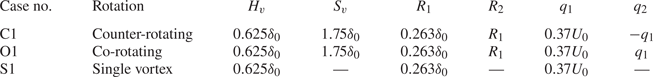
To start with, we compare three baseline cases, here referred to as case C1, the counter-rotating pair considered in § 4.1, case O1, which has the same set-up but with co-rotating vortices, and case S1, with a single vortex having the same strength and starting location.

4.2.1. Flow structure

Figures 11–13 display a visualisation of the flow in cases C1, O1 and S1, respectively. The plots include both $Q$-isocontours calculated from the instantaneous and time-averaged velocity:

(4.1)\begin{align} Q_{inst} &= \tfrac{1}{2} \left( (\boldsymbol{\nabla} \boldsymbol{\cdot} \langle \boldsymbol{u}_i\rangle)^2 - \boldsymbol{\nabla} \langle \boldsymbol{u}_i\rangle : \boldsymbol{\nabla} \langle \boldsymbol{u}_i\rangle^{\rm T} \right) , \end{align}

(4.2)\begin{align} Q_{mean} &= \tfrac{1}{2} \left( (\boldsymbol{\nabla} \boldsymbol{\cdot} \overline{\langle \boldsymbol{u}_i\rangle})^2 - \boldsymbol{\nabla} \overline{\langle \boldsymbol{u}_i\rangle} : \boldsymbol{\nabla} \overline{\langle \boldsymbol{u}_i\rangle}^{\rm T} \right) . \end{align}

Figure 11. Isocontours of the second invariant of the velocity gradient tensor ($Q$) for the C1 case. Mean flow contours are shown in red, and instantaneous contours are coloured blue and yellow for negative and positive spanwise vorticity ($\omega _z$), respectively.

Figure 12. Isocontours of the second invariant of the velocity gradient tensor ($Q$) for the O1 case. Mean flow contours are shown in red, and instantaneous contours are coloured blue and yellow for negative and positive spanwise vorticity ($\omega _z$), respectively.

Figure 13. Isocontours of the second invariant of the velocity gradient tensor ($Q$) for the S1 case. Mean flow contours are shown in red, and instantaneous contours are coloured blue and yellow for negative and positive spanwise vorticity ($\omega _z$), respectively.

Contours of $Q_{mean} = 2 \times 10^6$ are shown in red. These highlight the development of the mean vortices introduced by using the Batchelor vortex model as described in (2.2). The formation of a secondary, smaller vortex can be seen as the primary vortex interacts with the wall. Contours of $Q_{inst} = 1 \times 10^5$ are clipped to show only those where the mean spanwise velocity is $U_{z} > 5$ in the direction of the vortex, to highlight the instantaneous turbulent structures present over the top of the main vortex. The introduction of the turbulent structures at the inlet, and their interaction with the vortices, can be seen clearly. We also observe the formation of pairs of counter-rotating ring vortices, encircling the primary vortex highlighted in figures 11–13. These structures are coloured yellow and blue with positive and negative values of $\omega _z$, respectively. Initially, these ring vortices remain relatively coherent and grow in strength, before subsequently breaking down, due to both vortex–vortex and vortex–turbulence interactions. In the O1 case shown in figure 12, the two primary co-rotating vortices merge at location $\approx 15\delta _0$.

Figures 14(a,b) display the trajectories of the vortex cores from plan and side views, respectively. All vortices remain within the boundary layer for the full extent of the domain. As well as spreading apart, the counter-rotating vortices rise up within the boundary, although they do not rise as high as a single vortex, suggesting that the proximity to the counter-rotating vortex is holding them closer to the wall. The co-rotating vortices combine and migrate to one side, while they also rise significantly higher than the counter-rotating pair, before settling just below the edge of the boundary layer.

Figure 14. Trajectory of the vortex cores along the length of the developing boundary layer for cases C1, O1 and S1, for (a) plan view and (b) side view. The grey region at the start of the domain represents the SEM development region. In the side view plot, the boundary layer thickness ($\delta$) of an undisturbed boundary layer is shown in light grey for reference. (c) Integral of the positive shear stress over a plane. (d) Average shape factor along the length of the boundary layer. (e, f) Displacement and momentum thicknesses separately normalised by the case with no vortices present.

The shape factor $H$ is also plotted in figure 14(d) for these cases. This quantity, the ratio of the displacement thickness $\delta ^*$ to momentum thickness $\theta$, provides a measure of how close to the wall the momentum is contained. A lower value of $H$ therefore represents a more effective vortex generator configuration. Note that the quantity is averaged over a spatial region equal to the full $xz$ plane. It can be seen that the co-rotating pair, case O1, initially exhibits the lowest $H$, due perhaps to the movement of the smaller vortex towards the wall. At the point where the vortices merge, the co-rotating pair becomes less effective at transferring momentum to the vicinity of the wall, since the combined vortex settles in a location higher in the boundary layer than for the counter-rotating case C1. In all three cases, it can be seen that the shape factor is significantly lower than that of an undisturbed turbulent boundary layer. In the separate plots of displacement and momentum thickness shown in figures 14(e, f), respectively, it is shown that both thicknesses initially rise for the co-rotating and single vortices, whereas they initially drop for the counter-rotating case. This drop for the counter-rotating case can be attributed to the growing area of thinned boundary layer between the two vortices that is not present in the other cases. Case S1 is less effective at transferring momentum towards the wall, likely as with a single vortex the total circulation introduced is also lower. Figure 14(c) also displays a plot of the total positive shear stress over a plane, $\iint ( \overline {u'v'} )_{pos}$, along $x$, which is referred to later on.

4.2.2. Vorticity and shear stress

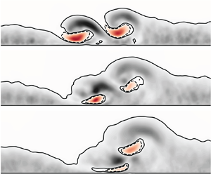
Figures 15–17 describe the downstream development of axial vorticity and both streamwise and spanwise shear stresses, for cases C1, O1 and S1, respectively. For case C1, shown in figure 15, the vorticity contours show how the primary vortices interact with the wall and generate secondary vortices near the wall. These secondary vortices are then pulled outwards and away from the wall by the primary vortices. The primary vortices reduce in strength and gradually move apart along the length of the boundary layer.

Figure 15. Contour plots for case C1, showing (a,d,g,j,m,p,s,v) the streamwise vorticity, and the turbulence shear stresses (b,e,h,k,n,q,t,w) $\overline {u'v'}$ and (c, f,i,l,o,r,u,x) $\overline {u'w'}$, with slices in the $yz$ plane taken at locations $x/\delta _0 =0, 2, 5, 10, 15, 20, 30, 60$.

Figure 16. Contour plots for case O1 showing (a,d,g,j,m,p,s,v) the streamwise vorticity, and and the turbulence shear stresses (b,e,h,k,n,q,t,w) $\overline {u'v'}$ and (c, f,i,l,o,r,u,x) $\overline {u'w'}$, with slices in the $yz$ plane taken at locations $x/\delta _0 =0, 2, 5, 10, 15, 20, 30, 60$.

Figure 17. Contour plots for case S1 showing (a,d,g,j,m,p,s,v) the streamwise vorticity, and and the turbulence shear stresses (b,e,h,k,n,q,t,w) $\overline {u'v'}$ and (c, f,i,l,o,r,u,x) $\overline {u'w'}$, with slices in the $yz$ plane taken at locations $x/\delta _0 =0, 2, 5, 10, 15, 20, 30, 60$.

The turbulence shear stress contour plots show that there is an area of considerable boundary layer thinning between the vortices. This is a good indication for the performance of the vortex generator in its ability to transfer momentum from the free stream closer to the wall and therefore delay the onset of potential separation. Also highlighted is the presence of an area of positive shear stress, shown in red. As discussed previously, this is an important factor in the preservation of the vortex, with the corresponding destruction of turbulence in the region slowing the diffusion of the vortex.

The contours of vorticity plots shown in figure 16 show a co-rotating vortex pair. In this case, both vortices initially move in the same direction before merging to form a single vortex from around $x=20\delta _0$. The merging of the vortices can also be seen in figure 14. It can be seen that the vortex starting at location $z = -7\delta _0/8$ is pulled closer to the other vortex whilst also descending lower within the boundary layer. Conversely, the vortex that starts at location $z=7\delta _0/8$ moves upwards. The lower vortex then passes underneath the other one before they combine at around $x=20\delta _0$. Once the vortices have merged to form a single vortex, it continues to slowly move away from the wall at a height larger than that of the counter-rotating pair but still within the height of an undisturbed boundary layer.

It can be seen from the contour plots of turbulence shear stress in figure 16 that at the point where the vortices merge, at $x=20\delta _0$, there is a significant drop in the positive shear stress. This is likely due to the increased shear flow that occurs as the two vortices approach each other. It can be seen in the contour plots in figure 16 that there is an area of strong, negative shear stress between the two vortex cores, supporting this hypothesis. In order to better assess this property, the shear stress is integrated in the area in the $yz$ plane where it is positive. This metric, $\iint ( \overline {u'v'} )_{pos}$, is then plotted against the streamwise direction and is shown for cases C1, O1 and S1 in figure 14. For the co-rotating vortex pairs, this shows a drop in positive shear stress as the vortices merge, followed by a significant rise.

4.2.3. Turbulence anisotropy and production

It is instructive to consider in more detail the nature of the observed levels of turbulence, both to aid the interpretation of the flow physics and to help us to understand RANS modelling of this flow. As discussed in § 1, previous attempts to use RANS models for these flows have demonstrated an inability to predict physics in the vortex core region. In this subsubsection, we consider the anisotropy of the turbulence, defined by

(4.3)\begin{equation} \boldsymbol{\mathsf{a}}_{ij} = \frac{\overline{\boldsymbol{u}'_i \boldsymbol{u}'_j} }{2k} - \frac{{\boldsymbol{\mathsf{\delta}}}_{ij}}{3}, \end{equation}

where ${\boldsymbol{\mathsf{\delta}}} _{ij}$ is the Kronecker delta function

(4.4)\begin{equation} {\boldsymbol{\mathsf{\delta}}}_{ij} = \begin{cases} 1, & \text{if } i=j,\\ 0, & \text{otherwise}. \end{cases} \end{equation}

Also presented is the production of the turbulence kinetic energy which is calculated as

(4.5)\begin{equation} P_k = \overline{\boldsymbol{u}'_i \boldsymbol{u}'_j}\,\frac{\partial \boldsymbol{U}_i}{\partial \boldsymbol{x}_j}. \end{equation}

In figures 18–20, we display these quantities for cases C1, O1 and S1, respectively. The anisotropy is plotted using the colour map method proposed by Emory & Iaccarino (Reference Emory and Iaccarino2014). In this method, the componentality of the turbulence anisotropy at each point of the domain is allocated an RGB colour by mapping the eigenvalues $\lambda _i$ of the anisotropy tensor ($a_{ij}$) onto a barycentric map and assigning an RGB colour value to each position on this map:

(4.6)\begin{equation} \left[ \begin{array}{@{}c@{}} {\rm R}\\ {\rm G}\\ {\rm B} \end{array} \right] = C_{1c}^*\left[ \begin{array}{@{}c@{}} 1\\ 0\\ 0 \end{array} \right] + C_{2c}^*\left[ \begin{array}{@{}c@{}} 0\\ 1\\ 0 \end{array} \right] + C_{3c}^*\left[ \begin{array}{@{}c@{}} 0\\ 0\\ 1 \end{array} \right], \end{equation}

where

(4.7a–d)\begin{align} C_{ic}^* = (C_{ic} + C_{off} ) ^{C_{exp}}, \quad C_{1c} = \lambda_1 - \lambda_2, \quad C_{2c} = 2(\lambda_2 - \lambda_3), \quad C_{3c} = 3\lambda_3 + 1. \end{align}

Figure 18. Contour plots for case C1 of (a,d,g) turbulence kinetic energy $k$, (b,e,h) production of $k$, $P_k$, and (c, f,i) anisotropy componentality. Slices are in the $yz$ plane at locations $x/\delta _0 = 5, 15, 30$.

Figure 19. Contour plots for case O1 of (a,d,g) turbulence kinetic energy $k$, (b,e,h) production of $k$, $P_k$, and (c, f,i) anisotropy componentality. Slices are in the $yz$ plane at locations $x/\delta _0 = 5, 12, 30$.

Figure 20. Contour plots for case O1 of (a,d,g) turbulence kinetic energy $k$, (b,e,h) production of $k$, $P_k$, and (c, f,i) anisotropy componentality. Slices are in the $yz$ plane at locations $x/\delta _0 = 5, 15, 30$.

The constants used to define the colour map are $C_{off} = 0.55$ and $C_{exp} = 5$, such that distinct colours represent the three corners of the colour map (red, green and blue representing one component, axisymmetric two-component and isotropic turbulent structures, respectively) and the transition areas (yellow, cyan and magenta representing two-component, axisymmetric contraction and axisymmetric expansion, respectively). For clarity, a threshold is applied so that only areas of the flow where $k/U_0 > 0.005$ are shown.

The contours of production in figure 18 show that in the initial development of the vortices, a ring of high turbulence kinetic energy production is formed around the centres of the two vortices. Further downstream, at $x=15\delta _0$, while the turbulence kinetic energy peaks at the centre of the vortices, a rapid drop in production is observed. Indeed, at the vortex core, the production takes small negative values, coloured red in the figure. This is due to the spatial lag between the Reynolds stresses and the mean strain field, and is a characteristic result of rotating turbulent flows. This leads to a reduction of turbulence in the core, which in turn helps to reduce diffusion and increase the coherence of the vortex structures downstream. This feature cannot be captured with standard, linear, RANS models without an appropriate correction term. In contrast to isolated vortices, the present configuration is more complex on account of the interaction of the vortex with the boundary layer, which provides a continual source of turbulence kinetic energy to the vortex core. The balance of these two effects is likely to be sensitive to the distance of the vortex from the wall, amongst other factors. This effect is also observed in the S1 case in figure 20, and in the O1 case in figure 19, where it peaks as the two co-rotating vortices approach each other before merging.

Switching focus to the anisotropy plots, it is notable, in the context of the previous paragraph, that standard linear RANS models will not be able to account for the spatial lag between Reynolds stresses and the mean strain field. Furthermore, in shear flows dominated as in the present case, they will be limited in their ability to discern Reynolds stress anisotropy, in effect limiting their applicability to the blue regions of the graph for most of this flow, in some cases possibly also part of the cyan and magenta regions. In contrast, red and green regions, respectively referring to one- and two-component states of turbulence anisotropy, are beyond standard linear RANS models. The green regions above the vortices in the anisotropy plots in figures 18–20 show how as the mean flow outside the boundary layer is pulled in by the vortices, significant areas of axisymmetric two-component turbulence are found. Much of the areas of high production, near the surface of the wall and around the centre of the vortices, corresponds to red regions of the anisotropy plot. These are areas where turbulence tends towards a one-component state that represent characteristic near-wall streaks. Similar observations are made for the three cases C1, O1 and S1, highlighting the modelling challenge presented to RANS models for flows of this nature.

4.3. Parametric variation

To demonstrate the flexibility of the methodology proposed in § 4.1, we proceed to examine a series of different configurations of vortex pairs. In the following we report general trends observed by varying separation distance and effective skew angle for counter-rotating vortices.

4.3.1. Separation distance

For both counter-rotating and co-rotating vortex pairs, the effect of the separation distance $S_v$ on the dynamics of the vortices was investigated. The vortex paths in the $xz$ plane are shown in figure 21. For the counter-rotating vortex pairs, the change in the separation distance at the inlet $S_v$ correlates to a similar change in the vortex separation as they spread apart along the length of the domain. For the co-rotating pair, the inlet separation distance greatly affects the merging of the vortices; the closer together the vortices begin, the sooner they merge.

Figure 21. Plots showing how the positions of the vortex cores in the $z$-direction vary along the length of the developing boundary layer. The vortex paths for a range of separation distances ($S_v$) are shown for (a) co-rotating and (b) counter-rotating vortex pairs.

The location in the streamwise direction at which the vortices combine affects the total circulation of the vortex. This can be explained by the corresponding drop in the positive shear stress. Figure 22 shows that at the point where the vortices merge, there is a drop in the total positive shear stress at the vortex cores. This then leads to a steeper drop in the total circulation, shown in figure 22 as the turbulence from the boundary layer acts to weaken the vortices. This in turn corresponds to a drop in the spanwise coefficient of friction ($C_{f_z}$) on the wall, as shown in figure 23.

Figure 22. Plots of (a) the integral of the positive shear stress in a plane, (b) total circulation over the length of the turbulent boundary layer, for co-rotating vortices with separation distances in the range $1.5 \leq S_v/\delta _0 \leq 2.5$.

Figure 23. Plots of coefficient of friction in (a,b) the $x$-direction, and (c,d) the $z$-direction, for co-rotating vortices with various separation distances $S_v$. Counter-rotating vortices are shown in (a,c), and co-rotating vortices in (b,d).

For separation distances $S_v = 1.5 \delta _0$, $1.75 \delta _0$ and $2.0 \delta _0$, there is a clear dip at the positive turbulence shear stress around the location where the vortices merge, followed by a substantial peak. However, for separation distances $S_v > 2 \delta _0$, the drop in $\iint ( \overline {u'v'} )_{pos}$ is far more gradual. At separation distance $S_v = 2.25 \delta _0$, the area of positive shear stress recovers after merging; however, for $S_v = 2.5\delta _0$, the integral drops to zero and no recovery is observed.

The effect of variable separation distance on the coefficient of friction at the wall is shown in figure 23, with both the streamwise ($C_{f_x}$) and spanwise ($C_{f_z}$) values plotted for counter-rotating and co-rotating vortices. For counter-rotating vortex pairs, a higher separation distance corresponds to a faster rise in $C_{f_x}$. Although a higher $C_{f_x}$ corresponds to a higher drag force acting on the surface, it also suggests a higher resilience to separation, and shows the vortex generators working more effectively over a longer length. Vortices starting closer together are initially less effective, although in these cases, $C_{f_x}$ increases to levels observed in other cases further downstream as the vortices spread apart.

4.3.2. Skewed flow

In many practical applications, vortex generators are subject to yaw of the incoming flow. This could be due to either the misalignment of the vortex generators during installation or variations in the flow during operation, such as a vehicle under cornering conditions. This yaw angle leads to an imbalance in the vortex strength in a counter-rotating vortex pair. When investigating the effect of yaw angle, Lögdberg et al. (Reference Lögdberg, Fransson and Alfredsson2009) found that increasing the yaw angle in $0 \leq \beta \leq \alpha$ led to a linear increase in the strength of one vortex and a linear decrease in the other, with the total circulation remaining broadly constant. Following this, the relative strengths of the vortices $q_1$ and $q_2$ were varied whilst maintaining the total strength $q_1 + q_2$, and it was taken that

(4.8)\begin{equation} \frac{q_1-q_2}{q_1+q_2} = \frac{\alpha}{\beta} . \end{equation}

Figure 24(a) shows how, by modelling the skew angle in this way, the average circulation over the full domain for the individual vortices follows a linear increase and decrease respectively with the total circulation remaining constant. This matches qualitatively the results of Lögdberg et al. (Reference Lögdberg, Fransson and Alfredsson2009).

Figure 24. Plots showing (a) the total circulation and the circulation of the contributing vortices, and (b) the difference in the average shape factor introduced by the change in angle over the whole domain as the skew angle $\alpha$ relative to the vortex generator angle $\beta$ is varied. Plots of the coefficient of friction in (c) the $x$-direction and (d) the $z$-direction, for counter-rotating vortices with skew angles in the range $\alpha / \beta = 0\unicode{x2013}1$.

Figure 24(b) displays how the angle of skew affects the total shape factor over the length of the boundary layer ($H_{av}$). To highlight the change corresponding to the angle, this is shown relative to the shape factor of the case at $\alpha /\beta = 0$ by plotting $H_{av} - H_0^{\circ }$. As the relative skew angle $\alpha / \beta$ is increased in the range $0 \leq \alpha / \beta \leq 0.6$, the shape factor stays relatively consistent, with a slight decrease from the level found with $0^{\circ }$ of skew. This shows that over this range of skew angles, the effectiveness of the vortex generator to transfer momentum towards the wall and therefore delay the onset of separation is resistant to skew angle. At skew angles where $0.8 \leq \alpha / \beta \leq 1$, there is an increase in the total shape factor of the downstream boundary layer that would correspond to a reduction in the vortex generator's effectiveness to delay the onset of separation. This step change in the performance of the vortex generator in $0.6<\alpha /\beta <0.8$ can also be seen in the coefficients of friction in figures 24(c,d). Here, two distinct groups can be seen in the behaviour of $C_{f_x}$ and $C_{f_z}$. For $0 \leq \alpha /\beta \leq 0.6$, higher values of $C_{f_x}$ and $C_{f_z}$ are displayed along the length of the domain, with a drop in both as $\alpha /\beta \geq 0.8$.