


1. Introduction
Debris-covered glaciers, which have a continuous mantle of rock debris over the full width of at least part of their ablation areas, are common in geologically young uplifting mountain ranges where rates of sediment input to the glacier surface are high (Reference KirkbrideKirkbride, 1993;Reference Shroder, Bishop, Copland and SloanShroder and others, 2000; Reference Racoviteanu, Williams and BarryRacoviteanu and others, 2008a, Reference Racoviteanu, Arnaud, Williams and Ordonezb). An expansion of the extent of supraglacial debris cover has been documented in many parts of the world as glaciers shrink and retreat due to climatic warming (Reference Stokes, Popovin, Aleynikov, Gurney and ShahgedanovaStokes and others, 2007;Reference Bolch, Buchroithner, Pieczonka and KunertBolch and others, 2008;Reference Kellerer-Pirklbauer, Lieb, Avian and GspurningKellerer-Pirklbauer and others, 2008;Reference Schmidt and NusserSchmidt and Nusser, 2009;Reference Shukla, Gupta and AroraShukla and others, 2009). The significant impact of extensive debris cover on glacier mass balance through both acceleration (thin, patchy debris) and reduction (debris thicker than ~-0.01-0.05m) of surface melting has been demonstrated through field, remote-sensing and modeling studies (Reference ØstremØstrem, 1959;Reference Nakawo and YoungNakawo and Young, 1981; Reference Mihalcea, Mayer, Diolaiuti, Lambrecht, Smiraglia and TartariMihalcea and others, 2006;Reference Nicholson and BennNicholson and Benn, 2006; Reference Brock, Mihalcea, Kirkbride, Diolaiuti, Cutler and SmiragliaBrock and others, 2010;Reference Reid and BrockReid and Brock, 2010;Reference LambrechtLambrecht and others, 2011). Debris-covered glaciers are important freshwater reservoirs in the major mountain ranges of Eurasia and North and South America (Reference Hewitt, Wake, Young and DavidHewitt and others, 1989;Reference Barnett, Adam and LettenmaierBarnett and others, 2005;Reference Scherler, Bookhagen and StreckerScherler and others, 2011) and it is important to monitor and understand changes that affect the ablation and mass balance of these glaciers.
Few existing distributed glacier ablation and mass- balance models account for the effects of debris cover on melt rates. The models that have been developed specifically for debris-covered ice require knowledge of the spatial distribution of debris thickness for application at the glacier- wide scale due to the strong dependence of ice melt rates on debris thickness (Reference Nicholson and BennNicholson and Benn, 2006;Reference Brock, Rivera, Casassa, Bown and AcunaBrock and others, 2007;Reference Reid and BrockReid and Brock, 2010). While semi-automated satellite-based techniques for mapping the distribution of debris on glacier surfaces have been developed (e.g. Reference Paul, Huggel and KaabPaul and others, 2004), estimating debris thickness, using both direct measurement and remote sensing, has proved to be problematic. Field-based mapping produces reliable point data, but suffers from the difficulty of obtaining a large enough sample to interpolate a sufficiently accurate debris- thickness map across an entire debris-covered zone and is unrealistic for application to large or many glaciers. Recently, thermal band satellite imagery has been used to map the spatial pattern of debris thickness based on the known dependence of debris surface temperature on its thickness in the range 0 to ~0.5 m (e.g. Reference Taschner and RanziTaschner and Ranzi, 2002;Reference Ranzi, Grossi, Iacovelli and TaschnerRanzi and others, 2004;Reference MihalceaMihalcea and others, 2008a,b). These studies rely on empirical relationships between debris surface temperature and debris thickness derived from extensive field measurements at the time of image acquisition. These empirical relationships are usually not transferable across time and space as temperature- thickness relationships need to be recalibrated for different meteorological conditions and glacier localities.
To overcome these limitations, the aim of this paper is to develop a more generally applicable method for mapping debris thickness from satellite imagery, through a physically based energy-balance approach. Such a method has not previously been used to estimate debris thickness on a glacier and this is therefore a developmental study focusing on the development, initial application and assessment of the approach. Terra Advanced Spaceborne Thermal Emission and Reflection Radiometer (ASTER) thermal observations are used, although the method should be equally applicable to any thermal band sensor mounted on a satellite, airborne or terrestrial platform. Surface temperature is the principal variable controlling the balance of energy fluxes at a supraglacial debris surface (Reference Reid and BrockReid and Brock, 2010) and can be measured at suitable spatial resolution from satellite imagery. The spatial distribution of clear-sky incoming shortwave radiation can be calculated very accurately on a mountain glacier (Reference HockHock, 1999; Reference Pellicciotti, Brock, Strasser, Burlando, Funk and CorripioPellicciotti and others, 2005). The other variables required in the calculation of surface energy fluxes such as air temperature and wind speed can be obtained from local or reanalysis meteors logical data. Hence, with a thermal satellite image obtained under clear-sky conditions and a snow-free target, it is possible to solve the surface energy balance in each image pixel and thus to find the debris thickness as a residual, given some plausible assumptions about the thermal proper ties of the debris. This method has the potential to map patterns of debris of up to at least 0.5 m thickness at a regional scale and to monitor its change over time, both in the future and into the past using available satellite image datasets. Thus, it can provide a valuable tool for water management, understanding glacier response to climate change and studies of supraglacial debris transport.
This paper presents a series of steps in model development and validation and concludes with some recommend diatoms for future work. First, a point model to determine debris thickness (d) is developed, utilizing meteorological variables collected at a weather station located on a glacier surface and an optimized value for the surface aerodynamic roughness. Second, the point model is applied to other sites on the glacier with known debris thickness. Third, a relationship to spatially extrapolate air temperature using surface temperature is developed, enabling the application of the model to the whole debris-covered zone under two different scenarios: (1) a flat glacier (FLATMOD), assuming a surface slope of 0° in each pixel, applicable when a digital elevation model (DEM) acquired close to the time of the thermal satellite image is not available; and (2) a sloping glacier (SLOPEMOD), where slope and aspect for each pixel are incorporated into the model using a recent accurate DEM of the study site, to account for variability of radiative fluxes between pixels. Next, both of these scenarios are applied to a second satellite image acquired during a different year to test model transferability under varying atmospheric and meteorological conditions. Model perform ance is evaluated using independent measurements of d.Finally, model sensitivity to its parameters and input variables is assessed.
2. Study Site: Miage Glacier
Miage glacier (45°47'30''N, 6°52'00''E) (Fig. 1) is a temperate glacier located on the Italian side of the Mont Blanc Massif in the western Alps. It is the largest (11 km) debris-covered glacier in the Italian Alps (Reference Pelfini, Santilli, Leonelli and BozzoniPelfini and others, 2007). Accumulation areas (3000-4800 m a.s.l.) are con nected to a 6 km long low-gradient (<10°) tongue by a series of steep tributary glaciers (Fig. 1). The glacier is extensively debris-covered from the snout at 1770 m a.s.l. to an altitude of ~2400ma.s.l. (Reference Deline and OrombelliDeline and Orombelli, 2005). Above 2400m a.s.l., debris cover is discontinuous except on two large medial moraines. Debris material is supplied mainly by rockfalls and avalanche events occurring at exposed headwalls between the tributary glaciers (Reference Pelfini, Santilli, Leonelli and BozzoniPelfini and others, 2007; Reference DelineDeline, 2009).

Fig. 1. Terra ASTER image (1 August 2005 visible/near-infrared (VNIR) band 1) showing Miage glacier and the locations of the automatic weather station and debris temperature and thickness measurements.
Debris thickness ranges from a few centimetres in the upper reaches to >1 m at the glacier terminus (Reference Brock, Mihalcea, Kirkbride, Diolaiuti, Cutler and SmiragliaBrock and others, 2010), but the modal debris thickness over much of the debris-covered area is ~0.2 m (Reference Thomson, Kirkbride and BrockThomson and others, 2000). Debris sizes range from millimetres to large boulders >1 m, which are distributed throughout the surface debris cover but are located mainly along the top of medial moraines and related to large rockfall episodes. Debris is typically well sorted vertically, with an open clast layer of cobble- to boulder-sized material overlying gravels and a base layer of sands and silts, with the lowest part of the profile normally saturated. Rock lithology is composed of gneiss, granite, rusted debris, schist, slate and tectonic breccia, and in most areas the surface lithology is a mixture of these rock types (Reference Brock, Mihalcea, Kirkbride, Diolaiuti, Cutler and SmiragliaBrock and others, 2010). Surface velocities on Miage glacier range from a maximum of 70 50 m a-1 at the tributary confluences, 50-60 m a-1 over the glacier tongue to 20 to <10 m a-1 on the terminal lobes (Reference Smiraglia, Diolaiuti, Casati and KirkbrideSmiraglia and others, 2000).
The development of Miage glacier into a debris-covered glacier has modified its recent dynamic behavior in comparison with other alpine glaciers, and it remains close to its Little Ice Age maximum extent despite recent thinning (Reference Pelfini, Santilli, Leonelli and BozzoniPelfini and others, 2007;Reference Diolaiuti, D'Agata, Meazza, Zanutta and SmiragliaDiolaiuti and others, 2009). Miage glacier is ideal for this study due to the large archive of available data, its accessibility and its size, which is representative of medium to large debris-covered glaciers.
3. Data Sources
3.1. Field data
Field data were collected during a series of campaigns carried out between June and September in 2005, 2006 and 2007.
-
1. Debris surface temperature was monitored at 25 sites spread across the debris-covered zone using thermistors (2005 only;Fig. 1).
-
2. Meteorological conditions for each season (incoming and outgoing long- and shortwave radiation fluxes, air temperature and humidity, wind speed and direction) were recorded using an automatic weather station (AWS) positioned on the lower section of the debris-covered zone at 2030 m a.s.l. (Fig. 1). Full details of the measure ments and sensor specifications are given in Reference Brock, Mihalcea, Kirkbride, Diolaiuti, Cutler and SmiragliaBrock and others (2010).
-
3. Debris thickness was measured in the field by digging through the debris layer to the ice beneath and recording its thickness, dmes. To obtain dmes over areas representative of 90 m x 90 m pixels from an ASTER (AST08) image, debris thickness was measured at 5 m intervals along a series of transects aligned north-south and east-west (locations C and E in Fig. 1 and Table 1). From these transect measurements the average and variance of debris thickness for each transect area was calculated for comparison with the ASTER model debris- thickness estimates. In addition, 39 debris-thickness measurements were made along shorter transects (locations A, B and D in Fig. 1 and Table 1) and at the 25 surface temperature measurement points spaced across the entire debris-covered zone (Fig. 1 ;Table 1).
-
4. Debris temperature was measured at the surface and base (ice-debris interface) and at intermediate depths of 0.24 and 0.48 m in a 0.72 m thick debris layer located at the lowest sample point on the southern lobe (Fig. 1) at 10min intervals throughout the 2005 ablation season using HOBO Smart Sensors (Onset Instruments).
Table 1. Field debris-thickness measurements in 2005, 2006 and 2007. Refer to Figure 1 for measurement locations. The varied length of transect arms in 2007 and the upper reaches in 2006 resulted from the presence of bare ice, ice cliffs and steep moraine slopes which prevented safe access

3.2. Remotely sensed data
Terra ASTER AST08 (surface kinetic temperature image) images were acquired for 1 August 2005 (Fig. 2) and 29 July 2004 (90 m spatial resolution) from the Land Processes Distributed Active Archive Center (LPDAAC). AST08 images were generated by the LPDAAC from level 1 thermal infrared (TIR) ASTER data (bands 10-14 of the ASTER sensor). A temperature emissivity separation (TES) algorithm was applied by the LPDAAC to the level 1 data after they had been corrected atmospherically (Reference TonookaTonooka, 2005), radio- metrically and geometrically (Reference Iwasaki and FujisadaIwasaki and Fujisada, 2005) using the standard correction methods of the LPDAAC for ASTER satellite data (Reference SakumaSakuma and others, 2005; http://asterweb.jpl.nasa.gov/data_products.asp).

Fig. 2. (a) Terra ASTER AST08 image showing thermal emissivity and (b) band 4 ASTER shortwave infrared (SWIR) image, both from 1st August 2005.
More recent images were not available due to extensive cloud and/or snow cover. The image from 1 August 2005 was selected for model development, and the 29 July 2004 image was used as an independent image for model testing. A DEM of the study site generated from airborne lidar surveys between July and October 2008, with a spatial resolution of 2.0 m and vertical accuracy better than 0.5 m, was provided by Regione Autonoma Valle d'Aosta (Fig. 3). The slope and aspect of each pixel were extracted from the DEM using standard procedures in ArcGIS software. These slope and aspect values were then resampled to 90 m spatial resolution.

Fig. 3. DEM of Miage glacier derived from airborne lidar survey supplied by Regione Autonoma Valle d’Aosta.
4. Penetration of Daily Temperature Cycles in Debris
Figure 4 shows the average daily temperature cycles in the 0.72 m debris layer over a fine period in late July (21-30 July 2005). Daily temperature cycles become damped and lagged with increasing depth but penetrate all the way to the debris-ice interface. This result corresponds with the earlier findings of Reference Nicholson and BennNicholson and Benn (2006) and Reference Conway and RasmussenConway and Rasmussen (2000) who recorded diurnal temperature cycles penetrating to depths of 0.45 and 0.75 m, respect lively, in supraglacial debris. Hence, debris surface tempera true is dependent on debris thickness up to at least 0.75 m, supporting the use of surface temperature to map patterns of supraglacial debris thickness.

Fig. 4. 2005 average daily temperature cycles over a 10 day period of fine weather (21–30 July 2005) at four levels in a 0.72m debris layer. The values show depth below the surface, and 0.72m is at the debris–ice interface.
5. Point Model
To determine debris thickness from ASTER AST08 thermal imagery, dsat, we developed a model that is based on solving the energy balance for a debris-covered glacier surface (Eqn (1)) in order to find the conductive heat flux in the debris, G, as a residual. Assuming the debris-ice interface is at 0°C, the equation for G can be rearranged to find debris thickness by substituting a value for debris thermal conductivity, K, and approximating the rate of change of heat stored in the debris, ΔD, as a fraction of G (Eqns (2-4)).
Simplifying for LH=0 and substituting ΔD = -FG:
where S and L are the net shortwave and net longwave radiation fluxes, respectively, His the turbulent sensible heat flux, LH is the turbulent latent heat flux, F is a dimensionless constant with value 0.64, K is the debris thermal conductivity (0.96 Wm-1 K-1 based on the mean of 25 measure ments at Miage glacier by Reference Brock, Mihalcea, Kirkbride, Diolaiuti, Cutler and SmiragliaBrock and others, 2010), Ts is the debris surface temperature (°C) and d is the debris thickness (m). All fluxes are in Wm-2 and considered positive when directed towards the surface.
LH can be ignored as debris surfaces are dry during the daytime in the ablation season except immediately following rain, which is unlikely to affect satellite imagery acquired under clear-sky conditions (Reference Brock, Rivera, Casassa, Bown and AcunaBrock and others, 2007, Reference Brock, Mihalcea, Kirkbride, Diolaiuti, Cutler and Smiraglia2010). Areas of very thin debris may be saturated at the surface, but in these areas the vapour pressure gradient between the surface and atmosphere will be weak due to the low surface temperature, so LH will generally be very small. ΔD cannot be calculated when only a single satellite image is available, since the rate of debris temperature change over time is not known. As the rate of warming or cooling of debris is dependent on the rate and direction of heat conduction in the debris, ΔD is strongly related to G and hence AD can be estimated as a fraction, F of G (Eqn (2)). In order to estimate the value of F, the magnitude of ΔDat the time of image acquisition (10.40 UTC) was calculated using 10 min interval measurements of debris surface temperature recorded at the AWS by a down-facing pyrgeometer (T s,rad) during the 2005 ablation season, following Reference Brock, Mihalcea, Kirkbride, Diolaiuti, Cutler and SmiragliaBrock and others (2010). Based on these data, the average ΔDat 10.40UTC under clear-sky conditions is equivalent to 0.64 of G. Hence, F= 0.64 is substituted in Eqn (4).
His calculated using the bulk aerodynamic method:

where ρ a is air density (1.26 kgm–3, adjusted for altitude, Cpis the specific heat capacity of air (1010 J–1 kg–1 K–1; Oke, 1987), kis von Ka´rma´n’s constant (k= 0.4), uis wind speed (m s–1), Ta is air temperature (8C), zis the height at which uand T a are measured or estimated (z= 2 m) and z 0 is the aerodynamic roughness length (m). The scalar length for heat, z 0t , is considered equal to z 0. The non-dimensional stability functions for momentum (Φm) and heat (Φh) are expressed as functions of the bulk Richardson number Ri b (Reference BrutsaertBrutsaert, 1982; Reference OkeOke, 1987):
-
stable case, with momentum forces dominating and Rib positive:
(6)
-
unstable case, with buoyancy forces dominating and Ri b negative:
(7)(8)
where gis gravitational acceleration (9.81ms–2). If a stability correction is not applied, Hwill be severely underestimated under the strongly unstable surface atmospheric conditions likely at the time of image acquisition (Reference Brock, Mihalcea, Kirkbride, Diolaiuti, Cutler and SmiragliaBrock and others, 2010).
In the initial point model stage, S, Land Hare calculated using direct measurements of S, L, T a, T s and uat the AWS at 10.40UTC on 1 August 2005. It is assumed that the ice– debris interface is at melting point, which is valid for the ablation season at Miage glacier (Reference Brock, Mihalcea, Kirkbride, Diolaiuti, Cutler and SmiragliaBrock and others, 2010), with a linear vertical temperature gradient within the debris layer. Reference Reid and BrockReid and Brock (2010) show temperature profiles in debris are close to linear during the middle part of the day, including the time of image acquisition. Although Figure 4 indicates the daytime temperature profile with depth is steeper at the surface than base of the debris, the type of sensor used overestimates temperatures by several degrees when exposed to strong insolation (by comparison with radiative surface temperature measurements) and the linear profile assumption results in overestimation of Gat the base of the debris of only up to 10–15Wm–2.
To test the performance of the point model for estimating d, it was applied at the AWS site using hourly interval measurements of input meteorological variables and T s,rad for the period 10:00–13:00 on 1 August 2005 (a period when a downward-directed Gflux and approximately linear vertical debris temperature gradient are likely to exist). z0 was varied between 0.001 and 0.16m to identify its optimal value. ΔDvalues were calculated from the T s,rad measurements following Reference Brock, Mihalcea, Kirkbride, Diolaiuti, Cutler and SmiragliaBrock and others (2010) since the empirical estimate of ΔD= 0.64Gapplies only to conditions at 10.40UTC and is unlikely to hold at other times of day due to variation in the rate and sign of temperature changes in the debris.
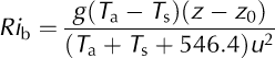
As can be seen in Figure 5, estimates of dcalculated using the point model are quite consistent over this period and show no temporal trend, providing support for the energybalance modelling approach. The time period shown covers contrasting meteorological conditions, including clouds and variable wind, demonstrating that the approach is quite robust to minor changes in meteorology.
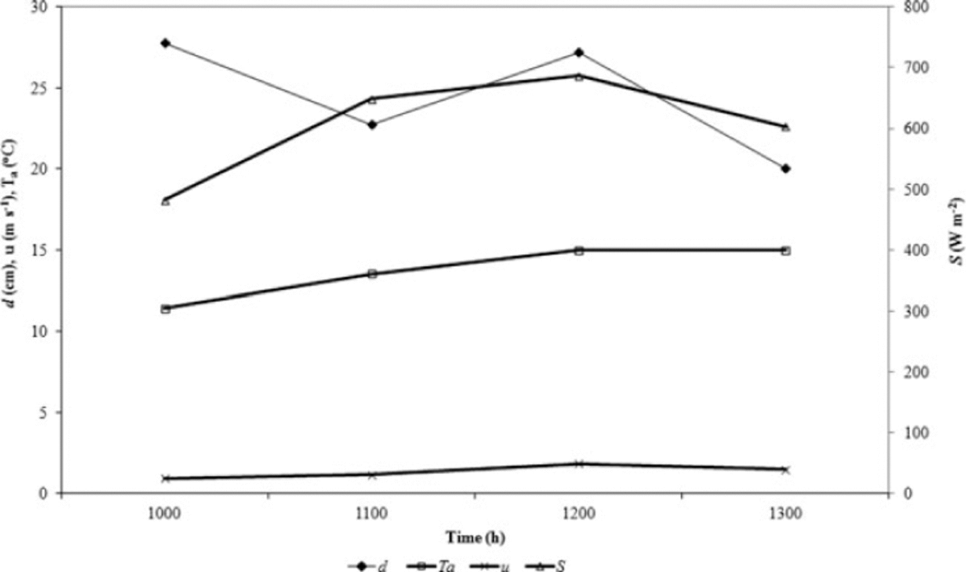
Fig. 5. Modelled debris thickness, d, at the AWS site on 1 August 2005 between 10:00 and 13:00 using measured input variables and z 0 = 0.006 m. dis the estimated debris thickness (cm), T a is the air temperature at 2m (8C), uis wind speed at 2m (m s–1) and Sis the net shortwave radiation flux (Wm–2).
Mean modelled debris-thickness estimates at the AWS on 1 August 2005 between 10:00 and 13:00 vary from 0.16m with z 0 = 0.003 m, to 0.15m with z 0 = 0.004m and 0.20m with z 0 = 0.006 m. These values agree well with a single point d mes of 0.16m recorded within the field of view of the downward–facing pyrgeometer and 0.23m at a stake adjacent to the AWS, although exact agreement with the point measurements should not be expected as this instrument is sensitive to radiation emitted from a large area (~10 m2) of debris. d is clearly sensitive to z0; unfortunately, little is known about the magnitude and spatial variability of z0 on debris-covered glaciers, and its value is estimated in the next section where the model is applied to the whole debris-covered zone of Miage glacier.
6. Point Model Application to Other Sites and Development of a Parameterization for Air-Temperature Extrapolation
To test the spatial transferability of the point model it was next applied to three sites on the glacier with known dmes using measured surface temperature from thermistors, T s,ther, as model inputs. These sites were at similar elevations to the AWS, so it was assumed that Ta at these sites would be the same as that recorded by the AWS.
However, the model was unable to estimate dmes, returning negative values at all three sites, most likely because the assumption that Ta is solely dependent on elevation, and would therefore be the same at sites of similar elevation, is false. All three sites had higher surface temperatures than the AWS, and inputting the T a value for the AWS in the model generated unrealistically large Hvalues in the range 586-839Wm-2, compared with 323 Wm-2 at the AWS, resulting in failure to find d. While understanding of the spatial variation of Ta across debris- covered glaciers is very limited, it is probable that T a is strongly related to T s during the morning under strong insolation conditions, as H and L are upwardly directed, transferring heat from the debris to the lowest layer of the atmosphere (Reference Brock, Mihalcea, Kirkbride, Diolaiuti, Cutler and SmiragliaBrock and others, 2010). Hence, Ts may be a stronger control on T a than elevation. In the absence of suitable data or models, the spatial distribution of Ta across a debris-covered glacier can be estimated from Ts.
As no distributed air-temperature measurements were available, the following empirical relationship between T a and Ts was developed based on a linear regression of 10 min interval values recorded at the AWS between 08:00 and 14:00 under clear-sky conditions during the 2005 ablation season:
where numbers in subscript are 95% confidence intervals for the two coefficients.
At wind speeds >5.9ms-1 the scatter in the relationship greatly increases, probably due to air being blown to the measurement site from off-glacier and the erosion of the glacier surface atmospheric layer. Hence, values recorded at u>5.9 ms-1 were not included in estimating the coefficients in Eqn (9). While there is some scatter in the T a-T s relationship (Fig. 6), the relationship is strong and linear (Eqn (9);r2 = 0.96, significance level <0.0001). Hence, the dependence of T a on T s is sufficiently strong to enable extrapolation of Ta based on Ts values in a distributed model. The strength of the relationship is indicative of the direct coupling between debris and air temperatures in the morning under clear-sky conditions when satellite images are likely to be acquired.

Fig. 6. Relationship of 2m air temperature to debris surface (radiative) temperature under clear-sky conditions between 08:00 and 14:00 recorded at the AWS during the 2005 season. The outer dashed lines are the 95% prediction intervals; 575 data points; 10 min average values. Data for days with wind speed >5.9ms–1 not included.
7. Model Application to the Whole Debris- Covered Zone Assuming a Surface Slope of Zero (FLATMOD)
The point model (Eqn (4)) was applied to the Miage glacier debris-covered zone using surface temperature values from the 1 August 2005 ASTER image (Tssat) with values of K = 0.96Wm-1 K-1 and F =0.64 to generate a single dsat estimate for each 90 m × 90 m pixel.
T a was calculated for each ASTER pixel by substituting Tssat into Eqn (9). Net shortwave radiation, S, incoming longwave radiation, L↓, and wind speed, u, were assumed to be equal to their respective AWS values in all pixels. Upwelling longwave radiation, L↑, was spatially distributed by estimating it from Tssat using the Stefan-Boltzmann relationship (Eqn (10)) with a debris emissivity of 0.94 (Reference Brock, Mihalcea, Kirkbride, Diolaiuti, Cutler and SmiragliaBrock and others, 2010):

where 0.94 is the average debris emissivity based on published values for granite and metamorphic rocks (Reference Brock, Mihalcea, Kirkbride, Diolaiuti, Cutler and SmiragliaBrock and others, 2010).
Values of z0 in the 0.001-0.016 m range were applied, since the typical range of gravel- to boulder-sized debris probably generates z0 values of the order of 0.001-0.01 m (Reference LettauLettau, 1969) and z0 = 0.016 m was obtained from analysis of a long period of profile measurements at Miage glacier in 2005 (Reference Brock, Mihalcea, Kirkbride, Diolaiuti, Cutler and SmiragliaBrock and others, 2010).
The most plausible results were produced for z0 values between 0.01 and 0.016m, with dsat generally increasing down-glacier in the 0 to 1 m+ range, broadly corresponding with the known pattern of debris-thickness distribution on the glacier (Fig. 7a). Thick debris on the medial moraines of the glacier tongue and an area of thin debris above the division of the northern and southern lobes are also correctly identified, but some features such as the area of thin debris along the southern margin of the northern lobe do not agree with visual observations. Use of z 0 values of <0.01 and >0.016 m resulted in unrealistic (values of tens of metres) d sat values.
Fig. 7. Estimated debris thickness (d sat) for the entire debris-covered zone using: (a) FLATMOD, 1 August 2005 ASTER image, z 0 = 0.016 m; (b) SLOPEMOD, 1 August 2005 ASTER image, z 0 = 0.016 m; (c) empirical equations from Reference MihalceaMihalcea and others (2008a) applied to 1 August 2005 ASTER image; (d) FLATMOD, 29 July 2004 ASTER image, z 0 = 0.016 m; (e) SLOPEMOD, 29 July 2004 ASTER image, z 0 = 0.016 m; and (f) empirical equations from Reference MihalceaMihalcea and others (2008a) applied to 29 July 2004 ASTER image. For the SLOPEMOD maps, 46 (z0 = 0.016 m) pixels use 08 slopes in 2005, and 51 (z 0 = 0.016 m) pixels use 0° slopes in 2004
8. Model Validation
8.1. Comparison with field measurements
Two sets of field transect samples taken in 2006 (locations C and E in Table 1 and Fig. 1) generated sufficient data to characterize d mes over areas large enough for direct com parison with dsat values (Table 2). The model closely matches dmes at location E, but underestimates it at location C. However, exact agreement between modelled dsat and dmes values should not be expected since, even using intensive field measurements, it is not possible to record dmes in all parts of the ground area covered by an ASTER pixel. Also, it is possible that there is some mismatch in the locations of the measurements taken in the field and satellite pixels.
Table 2. Comparison of average measured debris thickness (d mes) and debris thickness estimated from ASTER surface temperatures (d sat) at the two pixels corresponding to 2006 field dtransect measurements (Table 1) using the simple energy-balance model on 1 August 2005 (using z 0 = 0.01 and 0.016 m)
The mean modelled dsat for all 369 ASTER pixels closely matches the mean and range of values of the entire dataset of 224 field measurements made over the 2005-07 ablation seasons, particularly for z0 = 0.016 m (Table 3; Fig. 8a and c). Values of dsat are underestimated for z0 = 0.01 m, and z0 values >0.016m generate unrealistically large dsat values in pixels with high 7s. The shallow debris range 0.01-0.10 m is probably under-represented in dmes due to limited sampling in the upper zone of thin debris (Fig. 1), while debris much thicker than 0.50m was rarely recorded in dmes due to the difficulty of digging through very thick debris. Hence, while the field measurements cannot be taken as definitive 'proof' due to the representative sampling problem, the model's performance is generally supported by comparison with the field measurements.
Table 3. Comparison of descriptive statistics for all field transect and point measurements in the 2005–07 ablation seasons; d mes (n= 224; Table 1) and d sat estimated from FLATMOD and SLOPEMOD using the 1 August 2005 and 29 July 2004 ASTER images as input for different z 0 values (369 pixels). The 0.56m maximum dmes value is probably an underestimate of the true maximum debris thickness on Miage glacier. SD is standard deviation. For the SLOPEMOD data, 16 (z 0 = 0.01 m) and 46 (z 0 = 0.016 m) pixels use 08 slopes in 2005, and 20 (z 0 = 0.01 m) and 51 (z 0 = 0.016 m) pixels use slopes of 08 in 2004
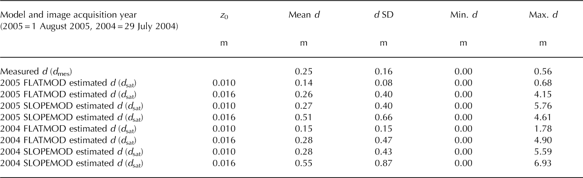

Fig. 8. Frequency histograms of: (a) all field debris-thickness measurements in 2005–07 (Table 1); (b) empirical equations published in Reference MihalceaMihalcea and others (2008a) applied to the 1 August 2005 image; (c) FLATMOD1 August 2005 image using z 0 = 0.016 m; (d) SLOPEMOD 1 August 2005 image using z 0 = 0.016 m; (e) FLATMOD 29 July 2004 image using z 0 = 0.016 m; and (f) SLOPEMOD 29 July 2004 image using z0 = 0.016 m. For the SLOPEMOD histograms, 46 (z 0 = 0.016 m) pixels use 08 slopes in 2005, and 51 (z 0 = 0.016 m) pixels use 08 slopes in 2004
8.2. Comparison with Mihalcea and others (2008a)
A previous debris-thickness map of Miage glacier was produced by Reference MihalceaMihalcea and others (2008a). They developed eight empirical equations for separate 100 m elevation bands based on the relationships between dmes and Tsther made simultaneously with the 1 August 2005 ASTER image at the 25 measurement points shown in Figure 1. Their debris-thickness map (Fig. 7c) provides a useful independent comparison for FLATMOD (Fig. 7a). The broad patterns of dsat are similar in both. FLATMOD identifies a larger area of very thin debris (<0.05 m) on the upper tongue, and thicker debris on parts of the terminal lobes and along the crest of the eastern medial moraine, where Reference MihalceaMihalcea and others' (2008a) dsat values are mostly <0.50m, despite the like lihood that mean thicknesses exceed this value in some pixels (Figs 7a and c and 8b and c). Reference MihalceaMihalcea and others (2008a) identify a large uniform area of medium-thickness debris (0.20-0.40 m) over the middle and lower glacier, where FLATMOD shows more variability in dsat. Overall, the close correspondence of the two dsat maps provides strong support for FLATMOD, particularly considering that the Reference MihalceaMihalcea and others (2008a) dsat map was generated from extensive field data and locally derived empirical relationships between debris thickness and surface temperature, while FLATMOD works independently of these data.
9. Incorporating Spatial Variability in the Shortwave Radiation Flux (SLOPEMOD)
FLATMOD can be applied when a high-resolution DEM acquired close to the time of the thermal satellite image is not available. To determine whether more accurate and detailed estimates of debris thickness could be obtained through a more realistic representation of the glacier surface (SLOPE- MOD), surface slope and aspect angles for each ASTER pixel were calculated from the 2008 lidar DEM and used to extrapolate shortwave radiation fluxes from the AWS across the debris-covered zone using standard geometrical calculations (e.g. Reference Brock and ArnoldBrock and Arnold, 2000) and an albedo of 0.13.
Spatial extrapolation of the flux of incoming longwave radiation, L↓, involves a significant degree of uncertainty in both the choice of parameterization and input data used (e.g. Reference Sedlar and HockSedlar and Hock, 2009), so the value recorded at the AWS using a high-quality instrument was applied to all parts of the glacier without adjustment. Upwelling longwave radiation, L↑, was estimated in the same way as in FLATMOD.
A problem occurred in the application of SLOPEMOD, as negative thickness values were calculated for 46 of the 369 pixels. These pixels are located on steep slopes (>20°) with high surface temperature (>25°C), mainly at the glacier margins but also on the sides of medial moraines and at known locations of large ice cliffs (Fig. 9). These unrealistic d values are probably a result of either geolocational errors, changes in surface topography over time, DEM and derived slope errors, or errors in flux calculations over steep slopes. To overcome this problem, the slope value was set to zero (i.e. the FLATMOD value) in these pixels and d recalculated.

Fig. 9. (a) Slope map derived from 2008 lidar DEM (2m resolution) and (b) plot showing location of negative debris-thickness estimates (d) from SLOPEMOD in 2005 (z0 = 0.016 m), which were subsequently set to the values obtained at corresponding pixels using FLATMOD.
The broad distribution of dsat from SLOPEMOD is very similar to FLATMOD (Figs 7a and b and 8c and d). SLOPEMOD identifies the same extent of thinner debris in the upper reaches and down the western side of the glacier. However, SLOPEMOD identifies several pixels with very thick debris (>1.0 m) in the middle and lower reaches of the glacier. These may reflect thick isolated piles of debris associated with periodic large rockfall events and more widely distributed thick debris on the terminal lobes, but it is unclear if the 'speckled' appearance of the SLOPEMOD map is due to improved model accuracy or modelling error associated with the DEM as discussed below.
The potential to apply SLOPEMOD using the global ASTER and Shuttle Radar Topography Mission 3 (SRTM3) (90 m) DEM products was explored. However, upon analysis, both datasets exhibited obvious inaccuracies with respect to elevation accuracy, resulting in large slope and aspect errors. Errors in the ASTER and SRTM3 DEM products caused by the steep mountainous terrain and resulting areas of shadow have been well documented (Reference KaabKaab, 2002, Reference Mihalcea2005; Reference Bolch, Kamp, Kaufmann and SulzerBolch and Kamp, 2005;Reference Racoviteanu, Manley, Arnaud and WilliamsRacoviteanu and others, 2007;Reference ToutinToutin, 2008; Reference Shortridge and MessinaShortridge and Messina, 2011) and these DEMs are generally unsuitable for application in SLOPEMOD.
10. Model Application To A Different (29 July 2004) Aster Image
To test the temporal transferability of the debris-thickness model and its applicability when no local meteorological data are available for the target site, FLATMOD was applied using a second ASTER AST08 image acquired in a similar midsummer period but in the previous year (29 July 2004). Changes in debris thickness on the glacier at the scale of an ASTER pixel are likely to be small over a 12 month interval, so similarity of the 2004 and 2005 debris maps can be taken as indicative of model transferability.
Surface temperature values from the two AST08 ASTER images were similar: 2004 (2005) mean 25.5°C (25.8°C), minimum 7.5°C (8.3°C), maximum 36.2°C (33.3°C). Meteorological values for u (12.00 UTC) and atmospheric precipitable water (day average;total atmospheric column) at Miage glacier on 29 July 2004 were obtained from US National Centers for Environmental Prediction (NCEP)/US National Center for Atmospheric Research (NCAR) reanalysis data (Reference KalnayKalnay and others, 1996). Values were interpolated to 2100 m (the median debris-zone elevation) from the 850 and 700mbar reanalysis levels without using ground control data. Incoming longwave and shortwave radiation were estimated from these data using the formulae of Reference Dilley and O'BrienDilley and O'Brien (1998) and Reference Strasser, Corripio, Pellicciotti, Burlando, Brock and FunkStrasser and others (2004), respectively. Equation (9) was used to distribute Ta across the debris zone from the Tssat values, and z0 values of 0.01 and 0.016 m were applied.
The d sat map generated from the 2004 ASTER image is very similar to the 2005 map, although dsat values are generally slightly lower over the tongue, but more areas of thick debris (>0.40 m) are identified on the lower glacier (Fig. 7a and d). Contrasting d sat values on the southern side of the northern lobe and the tip of the southern lobe in 2004 and 2005 may be the result of small patches of cloud which are apparent in the imagery (Fig. 2). However, the dsat range and mean are very similar in 2004 and 2005 (Fig. 8c and e; Table 3). Overall, these results support the application of FLATMOD in a 'data-poor' situation when meteorological data are obtained from reanalysis datasets, and also demonstrate the temporal transferability of the debris- thickness model.
SLOPEMOD was also applied to the 2004 image using the same DEM. Similar problems to the 2005 SLOPEMOD image were identified, with negative dsat values calculated in 51 pixels with steep slopes and high surface temperatures. These problems aside, the broad patterns, range and mean of dsat are very similar to the 2005 SLOPEMOD output (Figs 7b and e and 8d and f; Table 3).
Application of the Reference MihalceaMihalcea and others (2008a) model to the 2004 AST08 image generated a broadly similar map to the 2005 image, but a number of negative dsat values were generated (Fig. 7f). This illustrates that empirical models, which are highly calibrated to individual satellite images, are difficult to transfer to other satellite images, limiting their use for large-scale mapping and temporal- change studies.
11. Estimation Of Total Debris Volume On The Glacier
The total volume of supraglacial debris on the glacier was estimated using the histogram data in Figure 8 by multi plying each class frequency by the class midpoint debris- thickness value and then summing the values. The total volume estimates are 0.51-0.96 × 10⁶m3 using FLATMOD applied to the 2005 image, and 0.56-0.96 × 10⁶m3 using FLATMOD applied to the 2004 image, for z0 values in the range 0.01-0.016.
12. Sensitivity Analysis
The model inputs K, z0, F and Ta need to be calculated or estimated in the model. The values of the other meteoro logical input variables are also subject to uncertainty due to instrument and extrapolation errors. A sensitivity analysis was therefore conducted with the aim of identifying those variables and parameters that have the greatest influence on the value of dgenerated by the model, and hence should be priorities for further analysis to improve model perform ance. Using FLATMOD with the 1 August 2005 AST08 image as an initial run, the sensitivity of the mean d for the total debris-covered area to a ±20% variation in the input parameters and variables was calculated (Fig. 10).

Fig. 10. Sensitivity analysis. Variation of mean debris thickness in all 369 pixels for ±20% variation in input values. T a is the air temperature at 2m (8C), uis wind speed at 2m (m s–1), Sis the net shortwave radiation flux (Wm–2), T s is the debris surface temperature (8C), Lis the incoming longwave radiation flux (Wm–2), Kis the debris thermal conductivity, z0 is the aerodynamic roughness length and Fis a dimensionless constant used to estimate the flux of heat stored in the debris (ΔD).
Model sensitivity to Tssat is high, particularly since errors are amplified in the model through the estimation of Ta as a function of Tssat. The ASTER AST08 surface temperature products used in this study have an accuracy in the order of ±1.5 K and ±0.015 emissivity (Reference Gillespie, Rokugawa, Matsunaga, Cothern, Hook and KahleGillespie and others, 1998; Reference Sabol, Gillespie, Abbott and YamadaSabol and others, 2009), smaller than estimated in Figure 10 but still large enough to generate uncertainty in din the 0.05 0.10 m range. Of the four unmeasured input parameters/ variables, model sensitivity is very high to 7 a, moderate to z 0 and K, and low to F. The low impact of uncertainty in the value of F is reassuring given that the estimation of ΔD as a fraction of G is the biggest simplification of a physical process in the model. Although the sensitivity of dsat to variation in incoming S and L in Figure 10 is large, these variables can be modelled or measured with better than ±20% accuracy. Hence, model sensitivity to incoming S and L is considered to be small for the likely range of measure ment error. In contrast, the mean modelled dsat does show some variation for a probable underestimate of the un certainty in u, given that the assumption of spatial uniformity across the glacier is unlikely to be true. Model dependency on z0, Ta and u demonstrates the high sensitivity of the Hcalculation to small changes in conditions in the surface layer when the atmosphere is unstable. Future improvement to the model and its transferability will require further study of spatial variation of these variables across debris-covered glaciers and the magnitude of H at the time of image acquisition. Improved knowledge of the range and variability of K is also needed.
13. Discussion
The strength of the surface-temperature-based method of estimating d using a physically based model is illustrated in Figure 11. Ts is very sensitive to small variations in dbetween ~0.0 and 0.5 m, which is the critical thickness range for input to models of sub-debris ice melt rates. Ts varies more gradually for increasing d above ~0.5m, but variation in d is of relatively minor importance to variation in melt rates above this value. The influence of slope on the modelled dvalue is of minor importance on very thin debris, but has much greater influence for thicker debris when Ts>20°C.
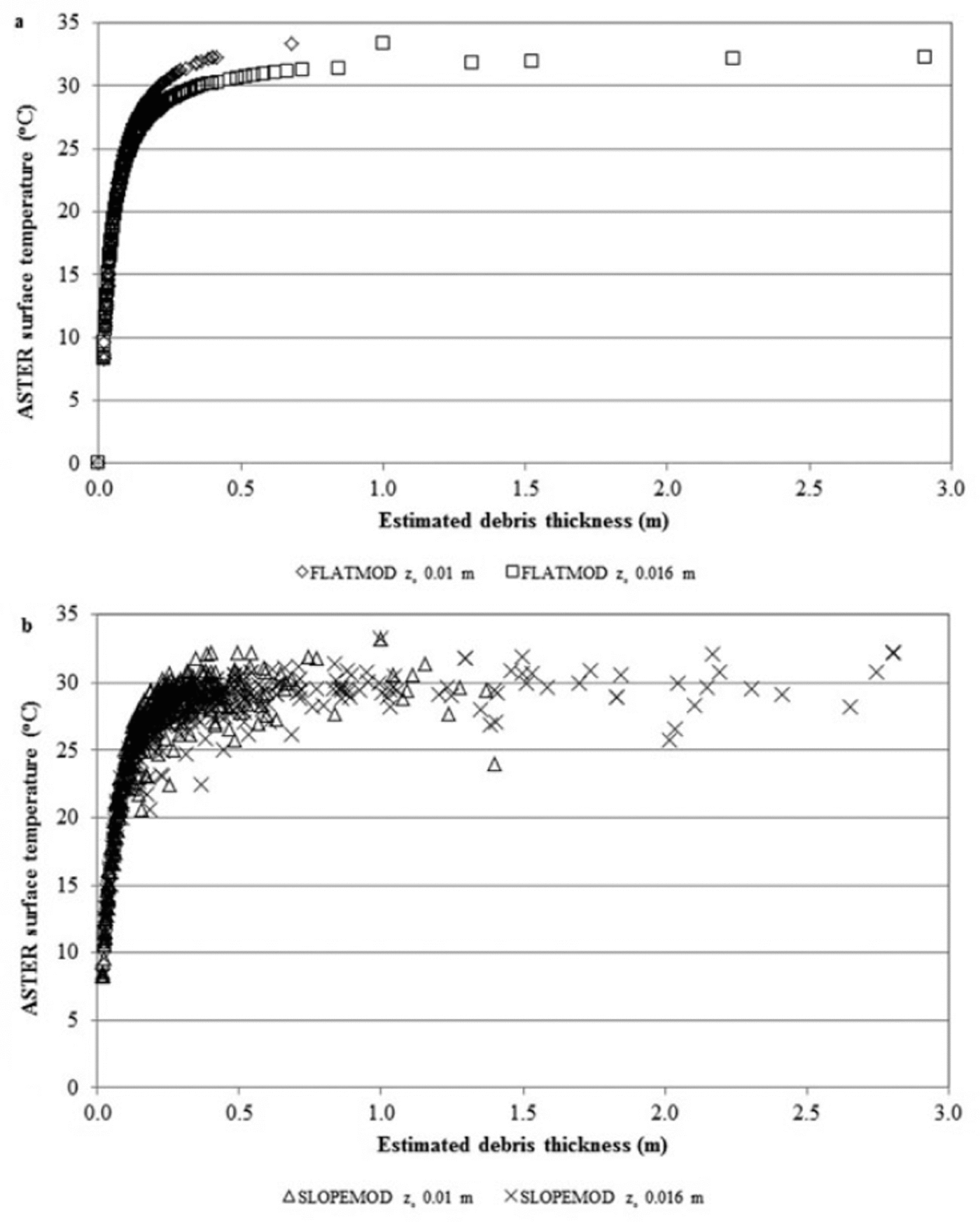
Fig. 11. Relationship of surface temperature from the ASTER 1 August 2005 image to debris thickness estimated from (a) FLATMOD and (b) SLOPEMOD using z0 values of 0.01 and 0.016 m.
To obtain debris thickness from an ASTER pixel we assume that temperature variations related to local topog raphy (variable slope and aspect) are integrated across a 90 m × 90 m pixel. Mixed debris and bare-ice pixels are inevitable in areas of patchy debris towards the upper limit of the debris cover. These are calculated as the lowest debris-thickness class (0.00-0.05 m) in Figure 7, indicating areas where debris is thin, patchy and potentially accelerating rather than reducing ablation. The key advantage of a physically based method over an empirical one is transfer ability in time and space without the need for recalibration. Owing to current poor understanding of several properties of supraglacial debris and the processes of energy exchange with the overlying atmosphere, the physically based model developed in this paper relies on several empirically derived relationships and values, which may not necessarily be transferable to other glaciers or times.
13.1. Aerodynamic roughness length, z0
There are few measurements of z 0 on debris-covered glaciers (Reference Takeuchi, Kayastha and NakawoTakeuchi and others, 2000;Reference Brock, Mihalcea, Kirkbride, Diolaiuti, Cutler and SmiragliaBrock and others, 2010), but variation in the value of z0 will be controlled by the lithologyand processes of emplacement, weathering and redistribution of the debris material, which affect the size and distribution of surface roughness elements. The typical range of gravel- to boulder-sized debris probably generates z0 values in the order of 0.001-0.01 m (Reference LettauLettau, 1969). As shown (Fig. 10), the model-derived value of d is quite sensitive to z 0, so measurements of z 0 on representative glaciers in different regions would facilitate successful application of the model to new sites. In contrast to clean glaciers, z0 is unlikely to show temporal evolution during the ablation season due to differential ablation features such as snow ablation hollows and ice hummocks.
13.2. Debris thermal conductivity, K
Values of Kfrom direct measurements (Reference Nakawo and YoungNakawo and Young, 1982; Reference Conway and RasmussenConway and Rasmussen, 2000; Reference Brock, Mihalcea, Kirkbride, Diolaiuti, Cutler and SmiragliaBrock and others, 2010) or estimated from physical constants for typical rock debris-forming materials (Reference Nicholson and BennNicholson and Benn, 2006) span almost an order of magnitude (0.47-2.60Wm-1 K-1), although some of this range can be explained by measure ment errors or unrealistic assumptions about the void space and moisture content of debris material. Reference Brock, Mihalcea, Kirkbride, Diolaiuti, Cutler and SmiragliaBrock and others (2010) found the range of Kon a single glacier to be much smaller (standard deviation of 0.20Wm-1 K-1), which generates an acceptable level of uncertainty in modelled d (Fig. 10) and justifies the use of a single value of K for an individual glacier.
Debris showed similar vertical profiles of size sorting and moisture content (as described in Section 2) at most of the 224 debris-thickness measurement points, even close to the upper debris limit. Hence, the processes of weathering, eluviation of fines and downslope transport of debris operate quickly to generate similar lithological properties across most of the debris zone. These properties, combined with the fact that suitable satellite input data will always be acquired under sunny ablation-season conditions, means that Kcan be estimated at unmeasured glacier sites with sufficient accuracy for derivation of d, provided the dominant rock types are known. Clearly, there are areas where Kmay differ more (e.g. areas of large boulders and thin and patchy debris), but in these areas the extreme high and low surface temperature values will lead to correct identification of thick and thin debris, respectively, in the model, regardless of the K value.
13.3. Magnitude of ΔD
The model assumption that ΔD is equivalent to a fraction, F, of the residual G flux (Eqn (2)) is necessary since satellite sensors cannot provide the two or more measurements of T s over a short time interval required to calculate ΔD directly, although this may be possible with airborne or terrestrial thermal measurements. While further study of the variation of ΔD with variation in meteorological conditions and debris thermal and physical properties is warranted, the low sensitivity of modelled d to the value of F justifies the simplified approach used here.
13.4. Spatial distribution of Ta and u
Knowledge of spatial patterns of Ta and u across glaciers, and across debris-covered glaciers in particular, is extremely poor, which presents a particular problem considering the high sensitivity of modelled d to the values of Ta and u(Fig. 10). Under the conditions of strong insolation and low wind speed which are typical of the late-morning acquisition of visible and thermal satellite imagery on alpine debris- covered glaciers, the surface atmospheric layer is warmed strongly by upwelling longwave radiation and sensible heat transfer from the underlying debris. Hence, it is likely that the spatial distribution of Ta correlates with Ts and, in turn, d,although the pattern will be complicated by horizontal air movement. This interpretation is supported by the analysis of Ta and Ts values recorded at the AWS (Fig. 6). These data were recorded on 16 days during July, August and September 2005 and show a remarkable consistency in the relationship of Ta to Ts on cloud-free mornings.
Hence, there is physical justification for the calculation of Ta as a function of Ts, although more measurements are clearly needed to determine whether similar relationships exist at other debris-covered glaciers. The assumption of spatial homogeneity in u is necessary given the lack of distributed measurements on glaciers. The limited under standing of spatial variation in Ta and u also presents a significant challenge for distributed energy-balance melt modelling of debris-covered glaciers, since the magnitude of H is extremely sensitive to the vertical temperature gradient and horizontal wind speed in the surface layer. Until more data and better glacier surface layer models become available, simplifying relationships such as Eqn (9) will need to be applied.
13.5. Spatial variation in incoming shortwave radiation and model sensitivity to small DEM errors
At image acquisition (10.40 UTC), the entire debris area is shadow-free. Variation in direct incoming shortwave radiation associated with decreasing atmospheric path length between the lower and upper debris limit elevations (~1800-2500 m a.s.l.) is very minor (<5Wm-2), meaning the value recorded at the AWS, close to the mid-debris elevation, is representative of the whole debris-covered zone under fine conditions when the diffuse shortwave com ponent of incoming radiation is small (15%). Differing amounts of terrain-reflected radiation may make variable contributions to total incoming shortwave radiation at different points on the glacier surface, but this component is very difficult to calculate accurately when the albedo at all points in the surrounding basin is unknown. Hence, the AWS recorded value of S was applied to all pixels, assuming a spatially constant albedo value (0.13). Reference Brock, Mihalcea, Kirkbride, Diolaiuti, Cutler and SmiragliaBrock and others (2010) found only minor spatial variations in dry debris albedo on Miage glacier, ranging from 0.12 to 0.16 in areas dominated by schist and by granite- and quartz-rich rocks, respectively. In most areas, the surface lithology is a mixture of these rock types, so the assumption of a constant albedo at the 90 m × 90 m pixel scale is generally valid.
The incorporation of spatial variability in incoming shortwave radiation as a function of surface slope resulted in a questionable improvement in model performance: identification of areas of thick debris (d> 0.50 m) but with some unrealistically high and negative d values generated. Generally, the more physically based a model becomes, the more it is affected by the quality of input data used. There is a greater risk of errors in d sat estimation when using SLOPEMOD due to errors within the DEM itself, incorrect geolocation (particularly at the glacier margins), changes to the glacier topography between the time of DEM and satellite image acquisition, and errors in flux calculations on steep slopes. Ideally SLOPEMOD would be applied when satellite and topographic data are acquired simultaneously at the same resolution. This was not the case in our study since the DEM was acquired during a series of airborne sorties in 2008 and does not match the time of the ASTER images. The differences in the detailed pattern of thick and thin debris in the 2004 and 2005 SLOPEMOD maps over the glacier tongue (Fig. 7b and e) probably result from the down- glacier movement of large debris mounds, with a scale of tens of metres in the horizontal and vertical, between the two epochs resulting in a different pattern of surface slope and aspect angles in 2004 and 2005. This demonstrates the high sensitivity of modelled d values to DEM errors. Owing to the tendency for debris-covered glaciers to develop long low-gradient tongues (Reference Paul, Huggel and KaabPaul and others, 2004), the FLATMOD 'flat glacier' assumption may well be a reasonable approx imation in the majority of cases, resulting in acceptably small errors in the S calculation.
14. Conclusions
This paper has described the development and testing of a physically based model to estimate supraglacial debris thickness using satellite thermal band imagery. The model is based on a solution of the energy balance at the debris surface in order to find debris thickness in each pixel as a residual. Required meteorological input can be provided from local observations or reanalysis data and the model can be run with or without a DEM of the target site. Hence, potentially it can be applied to map debris thickness across glaciers in remote areas without the need for field data. The sensitivity of surface temperature to debris thickness is greatest for shallow debris, so the model is best suited for mapping debris in the 0.0-0.5 m range. This is the critical thickness range for input to models of sub-debris melt due to the high dependency of melt rates on debris thickness up to ~0.5 m. The model is also able to identify areas with >0.5 m debris thickness, but with a high level of uncertainty in the exact thickness value. Hence, there is a limitation in the application of the model to map total debris volumes on glaciers with significant areas of debris >0.5 m thick (e.g. on large high Asian glaciers).
Validation of satellite-derived debris-thickness maps with field measurements is problematic due to the difference in scale between the ASTER AST08 pixels (90 m × 90 m) and point sampling on the glacier (< 1 m). However, satellite and field thickness estimates showed similar ranges for corresponding areas, and the satellite-derived maps correspond well with the known patterns of debris-thickness distribution on the glacier and with the published debris-thickness map of Reference MihalceaMihalcea and others (2008a). Furthermore, temporal transferability of the model was demonstrated through replication of results when applied to an earlier satellite image of the study site.
Owing to current lack of knowledge, a number of simplifying assumptions about debris thermal properties and meteorological variables across debris covers are made in the model. Based on a model sensitivity analysis, the most important uncertainties are in the spatial extrapolation of air temperature and use of a fixed value (not accounting for spatial variability) of both wind speed and aerodynamic roughness for all pixels. Studies of these variables are lacking, and future field measurements are needed to support the application of the debris-thickness model to other sites and also for the development of distributed energy-balance melt models for debris-covered glaciers. Field studies are also needed to improve understanding of debris thermal conductivity and the heat storage flux on different glaciers, although the model sensitivity to these variables is lower. The potential to utilize synthetic aperture radar (SAR) backscatter to characterize debris size and roughness should also be explored.
Knowledge of debris-thickness distribution is essential for realistic model estimates of global sea-level change and future water resources in major mountain areas such as the Hindu Kush Himalaya (Reference Scherler, Bookhagen and StreckerScherler and others, 2011). The method outlined in this paper offers the potential to provide the required debris-thickness data. As well as improving estimates of glacier melt and retreat under a warming climate, these could provide useful quantification of the reported expansion of debris covers on mountain glaciers (e.g. Reference Stokes, Popovin, Aleynikov, Gurney and ShahgedanovaStokes and others, 2007; Reference Shukla, Gupta and AroraShukla and others, 2009). In future studies we will apply the model to glaciers in different global regions and to thermal band remote-sensing data collected from airborne and terrestrial platforms.
Acknowledgements
This work was completed while Lesley Foster was in receipt of a studentship from the University of Dundee. It was supported by UK Natural Environment Research Council (NERC) grant NE/C514282/1, the British Council-Italian Ministry for University and Research (MIUR/CRUI) partner ship program and the Carnegie Trust for the Universities of Scotland. NCEP reanalysis data were provided by the US National Oceanic and Atmospheric Administration (NOAA)/ Office of Oceanic and Atmospheric Research (OAR)/Earth System Research Laboratories (ESRL)/Physical Sciences Division (PSD), Boulder, Colorado, USA, from their website at http://www.esrl.noaa.gow/psd. We thank C. Smiraglia, G. Diolaiuti, C. Mihalcea and C. D'Agata of the Department of Earth Sciences, University of Milan, and M. Vagliasindi and J.-P. Fosson of Fondazione Montagna Sicura, Cour- mayeur, for logistic support and help with data collection. The DEM was supplied by Regione Autonoma Valle d'Aosta. We thank Scientific Editor Ted Scambos and two anonymous reviewers whose comments on an earlier draft greatly improved the paper.


