


1. Introduction
The interaction between liquid droplets and solid surfaces is a widely investigated topic (Varagnolo et al. Reference Varagnolo, Ferraro, Fantinel, Pierno, Mistura, Amati, Biferale and Sbragaglia2013, Reference Varagnolo, Schiocchet, Ferraro, Pierno, Mistura, Sbragaglia, Gupta and Amati2014; ’t Mannetje et al. Reference ’t Mannetje, Ghosh, Lagraauw, Otten, Pit, Berendsen, Zeegers, van den Ende and Mugele2014; Sbragaglia et al. Reference Sbragaglia, Biferale, Amati, Varagnolo, Ferraro, Mistura and Pierno2014). Despite the apparent simplicity of the phenomenon, complex interactions occurring at the solid/liquid interface can result in counterintuitive behaviours (Liu et al. Reference Liu, Andrew, Li, Yeomans and Wang2015; Guzowski & Gim Reference Guzowski and Gim2019).
Liquid droplets impacting on solid surfaces are studied extensively since the resulting dynamics deeply influence a vast number of phenomena pertaining to scales ranging from micro (Seemann et al. Reference Seemann, Brinkmann, Pfohl and Herminghaus2011) to macro (Gent, Dart & Cansdale Reference Gent, Dart and Cansdale2000; Tokay, Kruger & Krajewski Reference Tokay, Kruger and Krajewski2001; Kinnell Reference Kinnell2005). Icing of supercooled water droplets, belonging to the latter set, represents a serious hazard to aircraft operational safety. Being triggered by the impact of high-speed travelling droplets with a solid surface (Lizer et al. Reference Lizer, Remer, Sobieraj, Psarski, Pawlak and Celichowski2017), icing is highly dependent on drop diameter and contact time between droplet and surface (Bird et al. Reference Bird, Dhiman, Kwon and Varanasi2013), therefore bouncing mechanisms and possible breakup are crucial aspects to be taken into account to reliably locate icing-prone areas. The case of flat solid surfaces, analysed deeply in the literature (Bobinski et al. Reference Bobinski, Sobieraj, Gumowski, Rokicki, Psarski, Marczak and Celichowski2014), covers only a small amount of possible interactions that can develop. Indeed, the growth of rime ice on fuselage and wings, triggered by water droplets hitting solid surfaces, starts at stagnation points like gaps and cavities. These aerodynamically quiet areas include flap hinges, control horns, fuselage frontal area, windshields, windshield wipers, wing struts, fixed landing gear, and gaps between panels. Remedies such as superhydrophobic coatings of solid surfaces (Cao et al. Reference Cao, Jones, Sikka, Wu and Gao2009) have been proposed widely, but the systematic prediction of a wide range of droplet dynamics is still needed.
The dynamics of droplets interacting with solid edges of orifices has been studied for low-impact (Reyssat et al. Reference Reyssat, Richard, Clanet and Quéré2010; Bordoloi & Longmire Reference Bordoloi and Longmire2014) and high-impact speed (Lorenceau & Quéré Reference Lorenceau and Quéré2003; Delbos, Lorenceau & Pitois Reference Delbos, Lorenceau and Pitois2010; de Maleprade et al. Reference de Maleprade, Bendimerad, Clanet and Quéré2021). The different regimes arising are due to the balance between inertia and gravity on one side, and surface tension and capillary forces on the other. These studies focus on impacts perpendicular to the orifice plane.
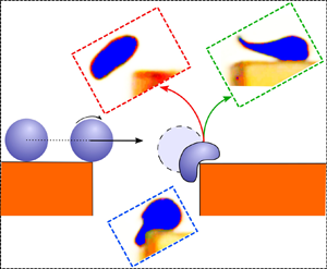
In this work, we explore a unique property of droplets running over a flat solid plane featuring a transverse gap. With reference to figure 1, the overall dynamics can be summarized as follows. A liquid of density  $\rho$, surface tension $\sigma$, is cast in the form of a drop of diameter $D$. The drop runs down an inclined plane, approaches the gap and takes off from the upstream edge of the gap with velocity $U_{I}$, flies towards the downstream edge, and possibly hits it. Impact features are fully determined at take-off time, therefore the impact is entirely described by the Weber number defined as
 \begin{equation} {We}=\frac{\rho U_{I}^2 D}{ \sigma}. \end{equation}
Figure 1. Sketch of the experimental apparatus showing the trajectory of a drop of diameter  $D$ running over an inclined plane of slope $\gamma$ approaching a gap of width $b$ with velocity $\boldsymbol {U}_{I}$ and rotational velocity $\omega _{I}$. Three different states are depicted: the drop takes off from the upslope edge (I), hits the downslope edge (II), and deforms as a consequence of the impact (III). The impingement on the downslope edge is indicated by a blue shaded drop, while the two trivial cases of falling and passing with no impingement are depicted by red and green shaded drops, respectively. The falling line $f$ is shown as a vertical green line passing through the downstream edge of the gap and ideally dividing the domain into upslope and downslope parts.
This study focuses on impacts able to extensively deform the drop. Indeed, the deformation is identified as the mechanism that allows the drop to climb the edge, whereas a rigid sphere of the same size, approaching the gap with the same kinematics, would instead have fallen down the gap. However, deformation alone cannot justify the peculiar ability to climb the edge; indeed, droplets sliding down a hydrophobic plane have been shown to develop a rolling motion (Richard & Quéré Reference Richard and Quéré1999; Reyssat et al. Reference Reyssat, Richard, Clanet and Quéré2010). Deformation, by inducing a sudden rise in contact area, promotes the conversion of the previously stored rotational momentum into an uplifting linear one. We employ an experimental set-up aimed at investigating a wide range of impacts by exploring different values of gap widths and, consequently, jump velocities to achieve a significant number of droplets impinging on the downstream edge of the gap. We interpret the data by means of an analytical model that simulates the asymptotic behaviour of an infinitely rigid droplet with vanishing  $We$ (i.e. a hard sphere). The differences between the drop and hard sphere behaviours emerge only in a specific range of $We$. The observed divergence between solid and deformable systems stands in clear contrast with previous studies where analogies between the two are hypothesized instead (de Maleprade et al. Reference de Maleprade, Bendimerad, Clanet and Quéré2021).
The paper is structured as follows. In § 2, the employed methodologies are described, namely the experimental apparatus, the energy balance approach and the analytical model of hard spheres. Section 3 is dedicated to the illustration and discussion of results. Conclusions and outlooks are drawn in § 4.
2. Methods
2.1. Experimental set-up
With reference to figures 1 and 2(a), the experimental set-up consists of an acrylic wedge fixed on a steel frame whose slope angle  $\gamma$ can be finely adjusted by means of an endless screw. Gaps of different widths $b$ have been carved on the wedge faces by means of a numerically controlled mill. To evaluate the sharpness of the edge, its radius of curvature has been estimated through stereo-microscopy to be $\eqsim 10^{-2}\unicode{x2013}10^{-3}$ times the drop diameter (see the supplementary material available at https://doi.org/10.1017/jfm.2022.750 for further details). The plane of motion can be divided into ‘upslope’ and ‘downslope’ parts by a vertical line (hereinafter referred to as the falling line $f$) passing through the downstream edge. It is worth highlighting that the gap width has been varied to achieve a significant number of droplets impinging on the edge. Indeed, such cases are the ones exposing the novel observed behaviour. The surface has been treated with a commercial coating (Ultra-Ever-Dry 2022), in order to obtain a hydrophobic surface. Measurements on the static contact angle provided a value $175^{\circ }$ for dyed (Methylthioninium chloride) tap water at room temperature (see figure 2b), which is the fluid employed in all the experiments. The measurement has been repeated during the experiment in order to rule out any change in hydrophobic properties. Throughout the study, surface tension is assumed to be that of undyed water. Dye concentration has been maintained constant throughout the whole experiment, to exclude any spurious effects on the surface tension and thus on the estimate of the Weber number. Small inaccuracies that may affect the estimation of the dyed water surface tension would then induce a uniform shift of the explored $We$ range.

Figure 2. (a) Experimental apparatus. The needle, fed by a modified medical syringe filled with the working fluid, is shown closer to the gap for the sake of clarity. (b) Graphical illustration of static contact angle measurement. (c) Typical evolution of a droplet jumping over the gap. Frames are not equally spaced in time; timing from the instant of jump is shown in each frame. A train of droplets is shown; the droplet under investigation is highlighted with a cross. Droplet trajectory is drawn as a dotted curve in all frames. The impact frame ( $t=9$ ms) is magnified and includes further information: the vertical line (falling line $f$) passing through the impact point is drawn as a dashed line; the red circle is the corresponding rigid sphere at the impact position – the sphere is not able to climb the edge, and bounces back with post-collision velocity $pcv$, denoted with a black arrow. The red arrowed line is the post-collision trajectory of the rigid sphere.
To achieve high-impact speeds (up to roughly  $1\,{\rm m}\,{\rm s}^{-1}$) over a small distance, the droplet generation has been obtained by placing a thin (22 gauge) needle parallel to the wedge face, pointing downslope, even though droplets on superhydrophobic inclined surfaces accelerate even faster than solid spheres (Reyssat et al. Reference Reyssat, Richard, Clanet and Quéré2010). The above set-up allows us to either gently release single droplets or shoot droplet trains with consistent initial speed.
Images of the droplets sliding down the wedge have been recorded by a 1000 frames per second (f.p.s.) side-mounted camera. See the supplementary material for explanatory movies of experimental runs. A mirror has been used to obtain a simultaneous top view of both the sliding and jumping phases. The scene is lit from both the opposite side of the camera and the bottom, taking advantage of the transparency of the acrylic wedge. Images have been analysed by means of in-house software tracking each individual droplet in the sequence. Pre-processing of acquired frames has been carried out in order to correct for focal distortion and remove the background. All the connected components (i.e. drops), identified through a segmenting procedure of the resulting image, have been detected, and a set of geometrical properties has been extracted for each one, namely centroid position, perimeter  $P$, and area $A$. A spherical-equivalent drop diameter $D$ has been determined by the analysis of a frame acquired during the drop jump over the gap, to exclude any deformation induced by the contact with the solid surface. A statistical analysis of the droplets’ circularity $\chi =4{\rm \pi} (A/P^2)$, evaluated at the same instant, yielded mean value $\mu =1.0062$ and variance $\sigma =0.0403$, confirming a negligible deformation during the jump.
2.2. Energy balance analysis
Drop deformation, as a consequence of the impact on the edge, causes a transfer from kinetic energy (both translational  $E_K^T$ and rotational $E_K^R$) to surface energy $E_s$. Both viscous $\Delta E_{\mu }$ and geodetic potential $\Delta E_g$ losses can occur during such evolution. With reference to figure 1, state I refers to the time of take-off, state II is the instant of first contact with the downslope edge, and state III is the instant of maximum deformation. A minimal energy balance across these three states can then be enforced. We assume that all the rotational kinetic energy is converted to other forms of energy during deformation. Such an assumption is justified by considering the large amount of deformation undergone during the impact, which is expected to strongly hamper the previously stored rotational motion. The assumption is supported further by the extremely low values of the residual translational kinetic energy at maximum deformation; indeed, a heavily deformed droplet, which also features a slow-moving centre of mass, is unlikely to possess a significant residual rotation. We assume that no viscous losses occur between states I and II (i.e. the flight duration). The formulation of the energy terms, employed to estimate the rotational energy, are listed in table 1, where $W$ is the drop volume; $\Delta h_{II}$ and $\Delta h_{III}$ are the losses in geodetic height between states I and II, and II and III, respectively; $\mu$ is the dynamic viscosity; $g$ is the gravitational acceleration; and $U_{I}$ and $U_{II}$ are the take-off and impact velocities, respectively. Quantities involved in the definition of energy terms for state III are defined as follows: $U_{res}$ is the residual velocity after deformation; $\Delta t$ is the time span required to achieve maximum deformation (state III) from the first contact with the edge (state II); $U_{def}$ is the characteristic velocity during the deformation process, defined as the average velocity over $\Delta t$; and $L_{def}$ is the characteristic size during the deformation process, defined as the minimum value of the drop thickness measured during deformation. The definition of $E_s$ at state III is based on the perimeter $C$ of the drop measured by image analysis at its maximum deformation.
Table 1. Energy content of each state:  $E_K^T$ is the kinetic translational energy, $E_s$ is the surface energy, $\Delta E_{\mu }$ is the viscous dissipation (the characteristic time scale is defined as $L_{def}/U_{def}$ by considering a dissipation function $\phi =\mu (\partial _jv_i+\partial _i v_j)\,\partial _j v_i \sim \mu (U_{def}/L_{def})^2$ as in Montessori et al. Reference Montessori, Tiribocchi, Bogdan, Bonaccorso, Lauricella, Guzowski and Succi2021), and $\Delta E_g$ is the loss of geodetic potential energy. The reader is referred to the text for the definitions of quantities appearing in the formulation of energy terms.

In order to evaluate the quantities needed to calculate the energy contributions at each state, the instants corresponding to the three states were determined on the basis of the kinematics of the drop. With reference to figure 3, states I and III occur when the drop is aligned with the upslope and downslope edges of the gap, respectively, and state II is assumed to be where  $U_z$, the velocity component perpendicular to the sloping plane, reaches its minimum value during the deformation process.

Figure 3. Example of (a) a trajectory of a drop and (b) its velocity component perpendicular to the sloping plane. Symbols pinpoint the three instants employed in the energy balance analysis: state I ( $\blacktriangle$), state II ( $\blacksquare$) and state III ( $\bigstar$). The drop at hand is one able to climb up after impinging onto the edge, as opposed to the corresponding sphere.
2.3. The analytical model for the impact of a hard sphere with the edge
To provide the reference asymptotic behaviour of a drop with vanishing  $We$ (i.e. large surface tension/vanishing velocity), an analytical model of both flight and purely elastic impact of a hard sphere has been developed. The accuracy of the model has been assessed by comparing its prediction with experiments on solid spheres (see § 3.1). With reference to figure 1, the trajectory of a hard sphere of diameter $D$, approaching a gap of width $b$ with velocity $\boldsymbol {U_{I}}$, can be predicted by integrating the two-dimensional equations of the motion accounting for the sole acceleration due to gravity. The formulation of the set of equations is reported in Appendix A. The impact with the downslope edge occurs when the latter is at a radius distance from the centre of the sphere. The sphere is assumed to undergo a purely elastic rebound as if it had hit the plane passing through the contact point with the edge. Moreover, the sphere, as well as the droplet, is assumed to fall in the gap if the rebound velocity vector, namely post-collision velocity $pcv$, lies in the ‘upslope’ midplane. This purely elastic energy-conserving impact stands as the asymptotic limit of the dissipative impact experienced by a deformable droplet. See Appendix A for a thorough description of the possible impact scenarios.
3. Results
3.1. Validation of the analytical model for hard spheres
The model described in § 2.3, though minimal, is proven to be able to predict accurately the fate of hard spheres analysed experimentally. The same experimental set-up has been used to perform further runs employing hard spheres rolling along the plane to gain the experimental data required to validate the analytical model reproducing the behaviour of a rigid body subject to the same dynamics as the drops. The employed hard spheres are plastic softair pellets of weight 0.16 mg with diameter  $D=5.7$ mm and density $\rho =1650\,{\rm kg}\,{\rm m}^{-3}$. Markers have been drawn on the spheres in order to quantify the amount of rolling motion before and after the impact. The measured angular velocity of the spheres ranged between $140\,{\rm rad}\,{\rm s}^{-1}$ and $190\,{\rm rad}\,{\rm s}^{-1}$, with results compatible with pure rolling motion with translational velocity $0.41\,{\rm m}\,{\rm s}^{-1}$ to $0.54\,{\rm m}\,{\rm s}^{-1}$.
The angle  $\alpha$ at which the drop approaches the downslope edge is given by the ratio of the two velocity components in the plane, that is, $\tan \alpha ={U_{x,{II}}}/{U_{z,{II}}}$. To quantify the agreement between analytical and experimental results of the hard sphere runs, experimental values of $\tan \alpha _{exp}$ have been measured for the impacts of the sphere and compared with the analytical ones ( $\tan \alpha _{{mod}}$). The comparison between $\tan \alpha _{exp}$ and $\tan \alpha _{mod}$ is shown in figure 4. To provide a clearer insight into how the model can predict the values of the impact velocity ${\boldsymbol {U}}_{{II}}$, the percentage difference between theoretical and experimental values of $\tan \alpha$ is shown in the scatter plot (figure 4). The agreement is remarkable, and allows us to rely on the results of the model. Measurements confirmed the rolling motion (the reader is referred to the supplementary movies) not changing before and after the impact, therefore ruling out any contribution of the rotational energy of the hard spheres to the ability to climb the edge. In other words, the model confirms that when no deformation occurs (i.e. punctual and instantaneous impact), no rotational momentum can be converted into enough vertical acceleration to make it to the other side of the gap. The results in figure 4 confirm further that the dynamics underlying the jump/fall behaviour of the rigid spheres is much simpler than that of the droplets, the former being determined by the approach angle alone.

Figure 4. Validation of the ballistic impact model for hard spheres: comparison between experimental and analytical values of the approach angle tangent  $\tan \alpha$. The inset reports the definition of both the approach angle and the velocity components $U_{x,{II}}, U_{z,{II}}$. The fate of the sphere is depicted by the different markers. Error percentage in the prediction of the approach angle is reported in the point labels. The dashed trace is the $45^\circ$ line.
3.2. Experiments on droplets
The experimental set-up is designed to be capable of generating a large amount of drops covering the portion of the diameter–velocity plane spanning roughly  $0.3\,\text {mm}< D<4\,\text {mm}$ and $0.19\,{\rm m}\,{\rm s}^{-1} < U_{I}<1.37\,{\rm m}\,{\rm s}^{-1}$. The investigated gap widths are $2.5\,\text {mm}< b<4.6\,\text {mm}$, and the slope angles are $6.7^{\circ }<\gamma <29.7^{\circ }$. The resulting $We$ covers two orders of magnitude, $0.5\lesssim {We}\lesssim 40$ (see the supplementary material for the complete dataset of experimental droplets). Given the investigated range of diameters, the resulting Bond number ( ${Bo}=\Delta \rho \, g(D/2)^2 / \sigma$), which compares the importance of gravitational to surface tension forces, falls within the range 0.003–0.5, therefore ruling out any substantial influence of gravity on the analysed dynamics. In the above, $\Delta \rho$ is the water–air density difference.
A statistical analysis has been carried out on  $1627$ droplets, employing a set of $We$ classes of uniform width $\Delta We=1$. The size and kinematics of each experimental droplet are also employed to run the analytical model for hard spheres. The outcome of the model, in terms of jump/fall behaviour, is then analysed with the same procedure as for the droplets.
For a discrete binary distribution, the success probability  $P_k$ of the $k$th class, i.e. the jump probability, can be constructed as
 \begin{equation} P_k=\hat{P}_k\pm z\,\frac{\sqrt{\hat{P}_k(1-\hat{P}_k)}}{\sqrt{N_k}}, \end{equation}
where  $N_k$ is the number of samples in the $k$th class, and $\hat {P}_k={n_k}/{N_k}$ is the success ratio, with $n_k$ being the number of successes. Since the number of droplets belonging to each class of $We$ is not uniform, a confidence interval is included in (3.1) in order to assess how significant the mean value is to describe the behaviour of each class, and $z$ is the quantile for the 95 % confidence interval (1.96 for the binary distribution).
3.3. Discussion
A typical evolution of an experimental run is depicted in figure 2(c), where nine frames of a train of four droplets are shown. The inner part of each droplet is highlighted in white for the sake of clarity. In the following, we focus on the second droplet, whose trajectory is drawn, featuring  $We=3$, which is able, after a considerable deformation, to climb the downstream edge of the gap and therefore make it to the other side. The centroid of the droplet under investigation in each frame is drawn as a cross. Up to the collision instant (i.e. $t=9$ ms), the sphere of equal diameter is also shown by a red circle. At the impact time, its post-collision velocity vector ( $pcv$) and post-collision trajectory, yielded by the analytical model, are depicted as a black arrow and a red arrowed line, respectively. Since the $pcv$ vector points to the left of the falling line, indicated at the impact time by a dashed line, the behaviour of this specific droplet differs from that of the corresponding sphere, which is not able to climb the edge.
The main finding of this study is condensed in figure 5, where the jump probability is plotted against  $We$ for droplets and hard spheres. Shaded areas indicate the $95\,\%$ confidence interval according to (3.1). The number of droplets available to the analysis for each class of $We$ class is also shown. It is clear that a range of $We$ exists for which a droplet exhibits a significantly higher probability of jumping over the gap. The upper bound of such range is roughly at ${We}=9$, while the lower bound (roughly ${We}=0.5$) is set by the employed experimental set-up: indeed, a way of consistently generating sub-millimetre slow droplets (i.e. low $We$) would be required while, at the same time, preventing them from bouncing instead of smoothly sliding/rolling over the inclined plane.

Figure 5. Empirical probability function of successful jump of droplets (black trace with triangles) and hard spheres (red trace with circles). Shaded areas represent 95 % confidence intervals. The dashed line with asterisks indicates sample size  $N$ for each $We$ class. There exists a range of $We$, roughly 0.5–9, where the liquid droplets develop a significantly higher probability of climbing over the downslope edge.
A further confirmation that the development of a rolling motion before the jump is the key feature for the ability to climb up the edge is given by the energy analysis. The balance described in § 2.2 can be employed to estimate the rotational energy at state I, which is assumed to be equal to that at state II:
 \begin{equation} E_K^R(\text{I})=E_K^T(\text{III})+E_{s}(\text{III})-E_K^T(\text{II})-E_{s}(\text{II})+\Delta E_\mu+\Delta E_g(\text{III}). \end{equation}
 The initial ratio of rotational to translational kinetic energy can then be plotted against  $We$ as in figure 6. Two sets of experiments are shown, both comprising drops which are able to climb up the edge: the first set, however, comprises the cases for which the corresponding spheres fall in the gap, while the second contains the remaining ones. By inspecting the mean values of the ratio, it is clear that the drops featuring a better ability to climb up the edge, compared to the corresponding hard spheres, are the ones that stored a higher rotational energy before the jump. Moreover, this analysis provides an explanation for the fact that, as shown in figure 5, the probability of finding a drop that develops the distinctive climbing ability is higher for low $We$; indeed, the energy balance suggests that such low-speed droplets are more prone to develop a rolling motion during the run over the sloping plane, as demonstrated by the markedly different slopes of the two fitting lines in figure 6. With reference to figure 6, it is worth mentioning that the droplets featuring a ratio $E^R_{K}/E^T_{K}>1$ at state I have been generated with a rotational speed larger than the speed of pure rolling. Such an occurrence is compatible with the employed method of droplets generation, i.e. ejection from a needle parallel to the sliding plane.

Figure 6. Scatter plot of the ratio of rotational to translational kinetic energy at state I ( $E_K^R/E_K^T$), as estimated by (3.2), versus Weber number; state I refers to the instant of take-off. Black circles filled with red indicate that the drop is able to climb up the edge while the hard sphere is not; hollow black circles indicate that both are able to climb. Lines are mean values and linear fits for the former (solid trace) and latter (dashed trace) subsets. The former subset features a higher fraction of rotational energy compared to the latter. Such a difference in stored rotational energy is more pronounced at low $We$.
$We$.
The energy balance also explains why the probabilities in figure 5 converge for high  $We$; indeed, the rotational energy is less prominent for high- $We$ droplets (see decreasing fitting lines in figure 6), which, in turn, develop a lower ability to jump the gap. In summary, the above analysis supports the initial conjecture that the different behaviour is triggered by the deformation, since the latter exposes a larger contact area, which, in turn, allows for the conversion of rotational to translational energy.
Moreover, our study contributes to the debate on the ability to develop rolling motion while sliding by droplets running over hydrophobic surfaces. Previous studies (Richard & Quéré Reference Richard and Quéré1999; Reyssat et al. Reference Reyssat, Richard, Clanet and Quéré2010) have shown a rolling behaviour at limit speed, and we show that such a limit speed is reached by droplets featuring a low  $We$ within the investigated range.
The dynamics observed in our experiment shows that between the two systems featuring the same amount of mechanical energy, namely the droplet and the hard sphere, it is the one able to enact a deformation process that has more chances to survive and maintain a higher gravitational potential energy.
4. Conclusions
In this work, a previously unexplored droplet dynamics has been investigated experimentally. A droplet faces a transversal gap while sliding/rolling over a hydrophobic plane, and possibly impinges on the downslope edge of the gap. The resulting deformation of the droplet allows for the previously stored kinetic rotational energy to be employed to climb up the edge. A critical Weber number exists, below which the droplet has a significantly higher probability of successfully jumping the gap compared to an equivalent hard sphere. An energy balance, carried out across the jump phases, shows that the ability to climb the edge is the result of the conversion of the rotational energy stored by the droplet before the jump. The deformation during the impact plays the main role in allowing such a conversion to occur.
The study provides novel quantitative observations of droplet dynamics interacting with geometric singularities of surfaces. Such geometric gaps are often found in many technical contexts, and comprehensive studies covering two order of magnitude of the Weber number are missing.
Supplementary materials and movies
Supplementary materials and movies are available at https://doi.org/10.1017/jfm.2022.750.
Acknowledgements
The authors are grateful to the three anonymous reviewers for their precious suggestions, to Professor M. Sebastiani (Roma Tre University) at DISSEMINATE laboratory for the stereo-microscopy assessment of edge sharpness, and to Professor E. Volpi (Roma Tre University) for stimulating discussions on the statistical analysis of the experimental data.
Funding
S.S. and A.M. are funded by the European Research Council under the European Union's Horizon 2020 Framework Programme (no. FP/2014-2020) ERC grant agreement no.739964 (COPMAT). V.L., M.L.R., A.M. and P.P. acknowledge funding from the Italian Ministry of Education, University and Research (MIUR), in the frame of the Departments of Excellence Initiative 2018–2022, attributed to the Department of Engineering of Roma Tre University.
Declaration of interests
The authors report no conflict of interest.
Appendix A. Hard sphere ballistic motion and purely elastic impact
With reference to figure 1, a sphere of diameter  $D$ rolls down the plane and approaches the upslope edge of the gap with velocity $\boldsymbol {U}_{I}=(U_{x,{I}},U_{z,{I}})$ (i.e. state I in figure 1). Neglecting the influence of the surrounding air, the subsequent motion is determined only by gravity, and can be described by the following set of equations:
 \begin{gather} x_{C}(t) =\tfrac{1}{2}\,g \sin(\gamma)\,t^2 + U_{x,{I}} t + x_{C}(0), \end{gather}
 \begin{gather}z_{C}(t) =\frac{D}{2}-\frac{g t^2}{2}\,\cos(\gamma) + U_{z,{I}} t + z_{C}(0), \end{gather}
where  $(x_{C}(t),z_{C}(t))$ is the position of the centre of the hard sphere at time $t$. The final terms of the right-hand sides of (A1) account for the initial actual droplet position at the frame where the centre is closest to the upslope edge. The impact instant (i.e. state II in figure 1) is then given by the lowest $\tilde {t}$ that satisfies the contact equation
 \begin{equation} \left(x_{C}\left(\tilde{t}\right)+b\right)^2+z_{C}\left(\tilde{t}\right)^2=\left(\frac{D}{2}\right)^2. \end{equation}
Once the impact time is found, the pre-collision velocity, i.e. the impact velocity  $\boldsymbol {U}_{{II}}$, can be estimated easily through differentiation of sphere position. With reference to figure 7, the post-collision velocity is found by mirroring $\boldsymbol {U}_{{II}}$ with respect to the line $r$ directed along the radius of the sphere passing through the edge of the gap. We refer to the vertical line passing through the edge of the gap as the ‘falling line’, namely $f$; the sphere is assumed to jump the gap if its post-collision velocity vector points to the right (downslope) of the falling line. Therefore, in order for the sphere to jump the gap, its impact velocity vector must lie within the shaded angle, bounded by the $x$ axis and the line $s$ obtained by mirroring the falling line with respect to $r$.
$r$.

Figure 7. Sketch of the framework employed to determine the fate of the rigid spheres. The blue circles depict two possible impact positions of a sphere;  ${f}$ is the falling line, i.e. the vertical line through the edge; the radius of the sphere belongs to the ${r}$ line; cases (a) and (b) differ by the position of the ${r}$ line with respect to the falling line; $s$ is obtained by mirroring the falling line with respect to ${r}$, and bounds the yellow shaded angle: any sphere whose impact velocity vector lies within such an angle is able to jump over the gap.


 Open access