


1. Two-dimensional turbulence and toroidal fusion plasmas
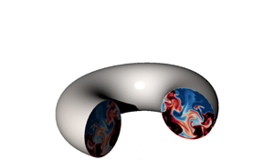
Thermonuclear fusion is a sustainable and carbon-free energy source. It can thereby constitute a game changer in the context of energy regulation and climate change. Currently the most advanced geometry to achieve the ultimate goal of a sustained large-scale fusion reaction is the tokamak: in a torus-shaped reactor chamber, magnetic fields are used to confine a plasma at a temperature of hundreds of millions of degrees, in which energy is produced by fusion of hydrogen isotopes. A schematic of the toroidal geometry, indicating the definitions of the toroidal and poloidal directions, is shown in figure 1.

Figure 1. Tokamaks are torus-shaped fusion reactors where the plasma is confined by a magnetic field. The toroidal component of the magnetic field is dominant in realistic reactors. In the simplified description considered here, we only consider this toroidal field and assume it to be strong enough to render the plasma-dynamics invariant along the toroidal direction. This reduces the dynamics to a two-dimensional (2-D) system, with three velocity components: two components in the poloidal plane,  $\boldsymbol u_P$, and one toroidal component $u_T$. In the present schematic we indicate the major and minor axes $R$ and $a$, respectively. The colour plot indicates the (toroidal) vorticity associated with the poloidal velocity field.
The largest obstacle for fusion is the confinement of a plasma. Indeed, if any reactor is to produce energy by a fusion reaction, the ionized gas of hydrogen isotopes should be kept at a sufficient temperature, with a sufficient density for a long enough period of time. This triple criterion (time, density and temperature) has been known since the 1950s (Lawson Reference Lawson1957) and the goal of almost any magnetically controlled fusion experiment is to enhance this triple product. Currently, tokamaks cannot work without continuous injection of energy in the plasma, and they produce less energy than they need to sustain the reaction. The ITER experiment aims at showing that tokamaks can reach, and go beyond, the break-even point.
The main factor limiting the confinement in tokamaks is turbulence. The transport of heat and matter by turbulent fluctuations degrades the confinement quality in all existing tokamaks (Liewer Reference Liewer1985; Garbet et al. Reference Garbet2004). The presence of some turbulence does seem inevitable given the enormous gradients of temperature and magnetic fields in the plasma edge, but limiting the intensity of this turbulence as much as possible in the reaction chamber is paramount. This explains the tremendous importance given to a transition between two turbulent states, observed first experimentally in the ASDEX experiment (Wagner et al. Reference Wagner1982). The transition from a highly turbulent, low-confinement mode (an L-mode) to a more quiescent, high confinement mode (H-mode), is observed to increase the confinement time considerably. Knowing how to trigger such a LH-transition, and keep a plasma in H-mode, can thus be essential for the design of a successful fusion reactor.
The understanding of the LH-transition is still incomplete. Different propositions of theoretical frameworks can be found in reviews on the subject (Connor & Wilson Reference Connor and Wilson2000; Wagner Reference Wagner2007). It is now well accepted that in H-mode, confinement is improved by the presence of shearing motion at the edge of the plasma (Shaing & Crume Reference Shaing and Crume1989; Groebner, Burrell & Seraydarian Reference Groebner, Burrell and Seraydarian1990; Shats et al. Reference Shats, Xia, Punzmann and Falkovich2007) and that interaction with the walls of the plasma vessel might play a role in this dynamics (Dif-Pradalier et al. Reference Dif-Pradalier2022). Such shearing motion allows us to decorrelate radially propagating structures by a mechanism called shear sheltering in the fluid mechanics literature (Hunt & Carruthers Reference Hunt and Carruthers1990; Hunt & Durbin Reference Hunt and Durbin1999). In the tokamak community this insight has had a major impact (Terry Reference Terry2000), in particular since magnetized plasmas show the formation of zonal flows, radially sheared poloidal flow structures, which contribute importantly to this shear sheltering (Biglari, Diamond & Terry Reference Biglari, Diamond and Terry1990; Diamond et al. Reference Diamond, Itoh, Itoh and Hahm2005; Gürcan & Diamond Reference Gürcan and Diamond2015).
Indeed, in addition to zonal flows, another established ingredient of the H-mode is its link with 2-D turbulence. It has been known since the works of Kraichnan (Reference Kraichnan1967) and Kraichnan & Montgomery (Reference Kraichnan and Montgomery1980) that a fluid flow in two space dimensions has the tendency to self-organize into large-scale structures. Examples of such self-organization are cyclonic structures in the atmosphere, and controlled numerical and physical experiments have verified this tendency to self-organization (McWilliams Reference McWilliams1984; Sommeria Reference Sommeria1986; Paret & Tabeling Reference Paret and Tabeling1997). The turbulence in plasmas seems to behave in a similar manner (Fyfe & Montgomery Reference Fyfe and Montgomery1979), i.e. the turbulence also tends to form large scale structures. This link between the formation of space-filling structures in 2-D flows and the H-mode was stressed in experiments (Shats, Xia & Punzmann Reference Shats, Xia and Punzmann2005). However, the magnetic field is also present in the L-mode, so that the dynamics should not be far from being 2-D. Therefore, it is not only the 2-D character of the flow which allows us to explain the LH-transition.
In the present study we use a representation of a toroidal plasma which is deliberately simplified as much as possible to study the dynamics of 2-D flow in a bounded toroidal geometry. Thereby we certainly miss a number of features that are important in describing the dynamics of fusion plasmas, but this approach allows us to understand a critical transition between nearly 2-D flow with three dominant flow components, to a purely 2-D flow and the influence of this transition on confinement properties. The present study is thereby complementary to investigations of simple models of plasma turbulence in periodic slab-geometry, such as the Hasegawa & Mima (Reference Hasegawa and Mima1978) and Hasegawa & Wakatani (Reference Hasegawa and Wakatani1987) models, which ignore the toroidal boundaries, while it remains simpler to interpret than toroidal simulations using the full three-dimensional (3-D) magnetohydrodynamics system or even more complex gyrokinetic descriptions (Grandgirard et al. Reference Grandgirard2006; Goerler et al. Reference Goerler, Lapillonne, Brunner, Dannert, Jenko, Merz and Told2011).
The motivation for the present work finds its origin in recent insights from theoretical studies on axisymmetric turbulence, which we will now briefly review. We consider purely axisymmetric flows, where not only the average flow quantities, but also every fluctuation is exactly axisymmetric. In the absence of magnetic fields or other body forces, in neutral fluids such a flow in the turbulent regime is difficult to establish. Therefore, in the fluid mechanics community, this type of flow has received interest only recently, mostly in order to extend ideas from statistical mechanics of 2-D flows to a case closer to three dimensions (Leprovost, Dubrulle & Chavanis Reference Leprovost, Dubrulle and Chavanis2006; Naso et al. Reference Naso, Monchaux, Chavanis and Dubrulle2010; Thalabard, Dubrulle & Bouchet Reference Thalabard, Dubrulle and Bouchet2014). Since such a turbulence is hard to reproduce experimentally, the assessment of theoretical ideas has been mainly achieved through direct numerical simulations of the axisymmetric Navier–Stokes equations (Qu, Bos & Naso Reference Qu, Bos and Naso2017; Qu, Naso & Bos Reference Qu, Naso and Bos2018). In a recent investigation (Qin et al. Reference Qin, Faller, Dubrulle, Naso and Bos2020) it was observed that a critical transition between two types of axisymmetric turbulence can be observed, where one of the flow states is characterized by typical 2-D behaviour, i.e. self-organization of large velocity structures, whereas the other flow is 2-D, but involves three velocity components (see figure 3c,d for an illustration). Even though this latter state is essentially 2-D, the large-scale flow structures are inherently unstable and tend to lose their energy to smaller scales, a feature reminiscent of 3-D turbulence: this change in cascade direction is a major difference between 2-D and axisymmetric 2-D three-component (2D3C) turbulence.
Whereas neutral fluid turbulence is rarely in a close to axisymmetric state, this changes for the case of electrically conducting fluids, or plasmas. Indeed, in the magnetohydrodynamic limit, the presence of a strong azimuthal magnetic field limits the variations in the direction of the field (Moffatt Reference Moffatt1967; Favier et al. Reference Favier, Godeferd, Cambon and Delache2010; Gallet & Doering Reference Gallet and Doering2015). In a tokamak, a strong toroidal magnetic field is present, which renders the flow close to axisymmetric. In general the strength of this field is an order of magnitude larger than the poloidal field (associated with a toroidal current) which we will neglect in our approach. The plasma in a tokamak is thereby close to a strictly axisymmetric state and can be described, at first order, by an axisymmetric fluid flow. We suggest that the transition which was discovered between two different axisymmetric turbulent states (Qin et al. Reference Qin, Faller, Dubrulle, Naso and Bos2020) should carry over to the dynamics of tokamaks. To illustrate this possibility, we have set up a numerical experiment in toroidal geometry and we will show the confinement properties of the two axisymmetric flow states from a pure fluid mechanics perspective.
We are not aware that such an elementary fluid set-up has been investigated previously. Most fluid mechanics studies in toroidal geometry have focused on liquid metal flows (Baylis & Hunt Reference Baylis and Hunt1971), and very few studies consider the axisymmetric limit (Poyé et al. Reference Poyé, Agullo, Plihon, Bos, Désangles and Bousselin2020). We think that, even if the transition that we will assess is shown in a too simple set-up to claim a one-to-one correspondence with the LH-transition, it does illustrate the robustness of the 2D3C to 2-D two-component (2D2C) transition in toroidal geometry, and its ability to dramatically change the flow physics and self-organization properties of the flow.
In the next section, we describe in detail the model we use to describe a turbulent plasma in toroidal geometry. In § 3 we discuss the numerical details. In § 4 we present the results of our numerical experiments. Finally in § 5 we conclude.
2. Modelling and governing equations
The system we consider is a model representation of a magnetically confined plasma in toroidal geometry. Since we assume axisymmetry, the dynamics can be described by a three-component dynamics in the poloidal plane. This simplifies the numerical experiments considerably. The poloidal domain on which we focus is shown in figure 2, where we indicate the coordinate system. The major radius is  $R$ and the minor radius $a$. The cylindrical coordinate system is centred around the major ( $z$) axis of the torus. In this coordinate system the radial and vertical directions in the poloidal plane are defined $r,z$. We also define a local coordinate system, centred in the circular cross-section, with polar coordinates $\rho,\theta$.

Figure 2. Spectral element mesh on the poloidal plane. The mesh consists of a central part and a boundary-adapted circular part. The major radius of the torus is  $R$ and the minor radius is denoted $a$.
$a$.
In the present section we will first introduce the fluid description. Then we will focus on the forcing protocol, representing the plasma instabilities, and we will explain how we measure the confinement quality of the plasma.
2.1. A fluid mechanics modelling of toroidal plasmas
Plasmas can be described by a hierarchy of physical models (Boyd & Sanderson Reference Boyd and Sanderson2003). The most precise, but thereby also least tractable, description is a kinetic approach involving all charged particles of the plasma and their non-local interactions (Diamond, Itoh & Itoh Reference Diamond, Itoh and Itoh2010). The coarsest approach is probably a fluid approach, where the plasma is described using continuum mechanics (Biskamp Reference Biskamp1997). In the present investigation it is this latter description which is adopted. We will omit all kinetic effects from our system. Furthermore, we will assume the dynamics to be isothermal, solenoidal and we do not model the detailed interaction of the plasma with electrical currents and magnetic fields. The only influence of magnetic fields which is retained in the present system is the influence of a toroidal magnetic field, assumed to be strong enough to render the dynamics perfectly axisymmetric. Physically this corresponds to the fact that charged particles can freely move along magnetic field lines, whereas perpendicular motion is constrained by Coulomb forces. This quasibidimensionalization of the flow is well documented in magnetohydrodynamical turbulence (Alexakis Reference Alexakis2011; Bigot & Galtier Reference Bigot and Galtier2011) and can even be exact when the magnetic Reynolds number is low enough (Gallet & Doering Reference Gallet and Doering2015).
In such an axisymmetric set-up, the dynamics are entirely described by the two velocity components in the poloidal plane  $\boldsymbol u_P=(u_r,u_z)$, and one component $u_T$ perpendicular to it (see figure 1). Such a system does not represent the instabilities associated with temperature, density and magnetic field gradients. In fusion plasmas, these gradients are at the origin of the turbulent fluctuations and these sources of instabilities are here modelled explicitly by appropriate external force terms.
We start by writing the axisymmetric Navier–Stokes equations:
 $$\begin{gather} \frac{\partial \boldsymbol{u}_P}{\partial t} +\boldsymbol{u}_P\boldsymbol{\cdot}\boldsymbol{\nabla}\boldsymbol{u}_P + \boldsymbol{\nabla} P-\nu\Delta\boldsymbol{u}_P = \boldsymbol{\mathcal{ N}}_P + \boldsymbol F_P , \end{gather}$$
 $$\begin{gather}\frac{\partial u_T}{\partial t} +\boldsymbol{u}_P\boldsymbol{\cdot}\boldsymbol{\nabla} u_T -\nu\Delta u_T = \mathcal{N}_T +F_T. \end{gather}$$
The pressure  $P$, in which we absorbed the constant density, ensures incompressibility through the condition
 \begin{equation} \frac{1}{r}\frac{\partial r u_r}{\partial r}+\frac{\partial u_z}{\partial z}=0. \end{equation}
The last terms on the left-hand side of (2.1) and (2.2) represent the viscous stresses, with  $\nu$ the kinematic viscosity. In these terms the $\varDelta$ indicates the axisymmetric vector-Laplacian in polar coordinates.
The left-hand sides of (2.1) and (2.2), respectively, describe purely 2-D fluid motion, represented by the velocity vector-field  $\boldsymbol u_P(\boldsymbol x,t)$ advecting the toroidal (out of plane) component of the velocity $u_T(\boldsymbol x,t)$. In a toroidal geometry the curvature introduces the $\mathcal {N}$ terms, which couple the two fields. The curvature terms are
 $$\begin{gather} \boldsymbol{\mathcal{N}}_P =u_T^2/r \boldsymbol e_r, \end{gather}$$
 $$\begin{gather}\mathcal{N}_T ={-}u_T u_r/r. \end{gather}$$
These terms are reminiscent of the vortex-stretching terms, essential in 3-D energy transfer, but absent in purely 2-D systems. All toroidal derivatives,  $\partial /\partial \phi$ are zero since we consider the axisymmetric case. Physically this assumption is justified by the presence of a strong toroidal magnetic field.
Before discussing the forcing terms  $\boldsymbol F_P$ and $F_T$, we will focus on the invariants of the system. In the absence of forcing and dissipation, the nonlinear interaction conserves a certain number of integral quantities. These quantities are not the same in the 2D2C or the 2D3C state. In the 2D2C case, the inviscid poloidal dynamics conserve the poloidal energy defined as
 \begin{equation} E_P=\tfrac{1}{2}\langle\|\boldsymbol u_P\|^2\rangle, \end{equation}
where the brackets denote a volume averaging. Furthermore, in this limit the enstrophy  $Z=\langle \|\boldsymbol {\nabla }\times \boldsymbol u_P\|^2\rangle$ is conserved. Furthermore, an infinite number of Casimirs (functions of the vorticity $\boldsymbol {\nabla }\times \boldsymbol u_P$) can be defined (Kraichnan & Montgomery Reference Kraichnan and Montgomery1980). These latter quantities play an important role in statistical mechanics, but are less important in determining the cascade directions of the system.
In the (curved) 2D3C case, the nonlinear dynamics conserve the total energy  $E_T+E_P$, where the toroidal energy is defined as
 \begin{equation} E_T=\tfrac{1}{2}\langle u_T^2\rangle. \end{equation}
The enstrophy is no longer a conserved quantity, but the helicity,
 \begin{equation} H=\langle (\boldsymbol{\nabla}\times\boldsymbol u) \boldsymbol{\cdot} \boldsymbol u\rangle, \end{equation}
becomes an invariant of the system. In cylindrical geometry (Qin et al. Reference Qin, Faller, Dubrulle, Naso and Bos2020), it was shown using energy and transfer spectra that the 2D3C–2D2C transition changes the cascade properties associated with the above invariants. The inverse transfer of poloidal energy  $E_P$ in the 2D2C case changed towards a direct transfer of the total energy $E_P+E_T$ to small scales in the 2D3C configuration. The assessment of energy cascades and fluxes is less convenient in the present set-up since we will consider solid boundaries and spatially localized forcing terms. We will therefore focus on a physical space characterization of the system.
An interesting feature is that, when the major radius of the torus tends to infinity (more precisely the ratio  $R/a$, see figure 1), the curvature and the associated $\mathcal {N}$ terms tend to zero. The axisymmetric 2D3C system tends to a Cartesian 2D3C system where it is no longer the total energy which is conserved, but $E_T$ and $E_P$ are conserved independently, and the poloidal dynamics behave as in the 2D2C case. In such a 2D3C geometry, the helicity degenerates to a correlation between the toroidal vorticity and the toroidal velocity, a quantity recently investigated in Linkmann, Buzzicotti & Biferale (Reference Linkmann, Buzzicotti and Biferale2018) and Yin et al. (Reference Yin, Agoua, Wu and Bos2024). It is not known at present how large $R/a$ must be to neglect the transfer. However, in the present investigation we will not vary the geometry, and the $\mathcal {N}$ terms cannot be neglected. The transfer between the components is thus possible and the total energy is an inviscid invariant of the system.
2.2. Forcing protocol
An important feature associated with a heated magnetized plasma is the presence of a number of instabilities leading to the generation of turbulent fluctuations. The forcing terms  $\boldsymbol F_P$ and $F_T$ are added to our system to reproduce the main features of sources of turbulent fluctuations in realistic plasmas (such as the interchange instability (Boyd et al. Reference Boyd and Sanderson2003)), which are located at the tokamak edge, where the pressure, density and temperature gradients are large. Modelling the ensemble of these instabilities together by artificial force terms might not represent certain important features associated with the feedback between the flow and the forcing, and this is necessarily left for future study.
To generate the poloidal velocity fluctuations, we add a Rayleigh–Bénard type instability as follows. We compute the advection of a scalar-field by the poloidal velocity field,
 \begin{equation} \frac{\partial b }{\partial t}+\boldsymbol u_P\boldsymbol{\cdot} \boldsymbol{\nabla} b=\kappa \Delta b +S'. \end{equation}
The term  $S'$ represents a source of scalar in the edge region of the plasma. More precisely, the value $S'$ is constant and is non-zero only in a shell near the boundary. The boundary condition at $r=a$ is the Dirichlet condition $b=0$. Thereby, on average a negative radial gradient builds up between the radial location of the source term and the boundary. The poloidal forcing term is
 \begin{equation} \boldsymbol{F_{P}}=C_{P}b\boldsymbol e_\rho+\boldsymbol F_\beta. \end{equation}
The first term in this expression leads then to the Rayleigh–Bénard-type (linear) instability, through the coupling of the poloidal velocity (i.e. (2.1)) and the scalar (i.e. (2.9)).
The second term,  $\boldsymbol F_\beta$ is a symmetry-breaking term, reminiscent of the anisotropic nature of a magnetized plasma. Indeed, in magnetized plasmas, a natural tendency to organize into concentric, toroidally invariant structures is observed related to the radial density gradients. The resulting zonal flows are equivalent to the zonal flows in rapidly rotating flows, such as the bands on Jupiter or Earth. To mimic this effect in the present set-up a body force is added to the poloidal forcing in the spirit of the Hasegawa–Mima equation (Hasegawa & Mima Reference Hasegawa and Mima1978; Gürcan & Diamond Reference Gürcan and Diamond2015):
 \begin{equation} \boldsymbol F_\beta =\beta' \rho\boldsymbol e_T \times \boldsymbol u_P. \end{equation}
This contribution to the poloidal force therefore does not inject energy in the system. As we will see below, the  $\boldsymbol F_\beta$ term is not essential to trigger the transition from 2D3C to 2D2C, but it leads to enhanced confinement if the transition to a 2D2C state is obtained. Simulations with and without this force will be presented.
The toroidal fluctuations are also assumed to originate from a linear mechanism and are simulated by a linear forcing term. More precisely, for the toroidal forcing we use
 \begin{equation} F_T=C_T\left[u_T-\tau_\sigma^{{-}1}\frac{\langle u_T r\rangle }{R}\right], \end{equation}
and it is applied on the same shell as the source term  $S'$. The notation $\langle {\cdot } \rangle$ indicates a spatial average over the poloidal domain. The second term allows us to avoid the build-up of toroidal angular momentum. Indeed, the spontaneous generation of angular momentum $\langle u_T r\rangle$ (or spin-up) in the system is of major interest (Rice et al. Reference Rice2007), but we want to disentangle this effect from the investigation of the transition between 2D2C and 2C3C flows. The present form of the toroidal forcing term does, therefore, dominantly excite the toroidal velocity fluctuations avoiding the build-up of mean angular momentum. In plasma experiments, a transition to a 2D2C flow, like the one we discuss here, might be accompanied by a global rotation associated with this angular momentum, which makes the identification of the transition less trivial.
2.3. Passive tracer to measure confinement
Eventually, we are interested in the confinement quality of the plasma. In practice, a good confinement in our system is associated with a small value of the radial turbulent diffusion. To measure turbulent diffusion, a passive tracer is injected continuously in the centre of the domain, while homogeneous Dirichlet conditions are imposed on the wall. The quantity  $\xi$, which follows the flow as a small amount of ink in a water flow, does not affect the flow, but allows us to measure the diffusion associated with the turbulent fluctuations. The governing equation is, as (3.4), an advection–diffusion equation,
 \begin{equation} \frac{\partial \xi }{\partial t}+\boldsymbol u_P\boldsymbol{\cdot} \boldsymbol{\nabla} \xi= \kappa\Delta \xi + f_\xi, \end{equation}
where  $f_\xi =C_\xi X(\rho _\xi -\rho )$, where $X$ is the Heaviside function, $\rho _\xi$ the radius of the source and $C_\xi$ a constant. When the turbulent fluctuations are strong, the diffusion allows efficient transport of the scalar, thus bad confinement, and the temperature in the centre of the domain drops. Thereby the centre temperature ( $\xi (\rho =0)$) directly measures the confinement quality of the flow. In the remainder of this article, we will call the scalar $\xi$ temperature, since we introduce it to measure the confinement of heat by the system. It is important to distinguish it from the other scalar $b$, associated with the poloidal forcing, since in our numerical set-up we decouple the dynamics of both scalars. This decoupling is voluntary here since we want to independently measure the confinement and adjust the forcing terms. In a fusion plasma the improved confinement of heat will necessarily lead to modified temperature gradients in the plasma, so that confinement and forcing are there coupled.
3. Normalization and numerical set-up
Before performing the numerical simulations, it is convenient to introduce an appropriate normalization of the governing equations. This allows us to identify the key parameters that will be varied. In this section we discuss the non-dimensionalization, the parameters used in our simulations and the numerical method.
3.1. Dimensionless equations
In order to non-dimensionalize the equations, we choose as a typical time scale the inverse of the poloidal forcing rate  $T^*=C_P^{-1}$. As length scale we use the minor radius $L^*=a$. This allows us to normalize the equations using $\tilde u=u T^*/L^*, \tilde {\boldsymbol {\nabla }}=L^* \boldsymbol {\nabla }$, and analogous for $\Delta,P, b,\rho, \partial _t$. Removing after normalization all tildes, for notational ease, we obtain the non-dimensional set of equations,
 \begin{align} \frac{\partial \boldsymbol{u}_P}{\partial t} +\boldsymbol{u}_P\boldsymbol{\cdot}\boldsymbol{\nabla}\boldsymbol{u}_P + \boldsymbol{\nabla} P-\frac{1}{Re}\Delta\boldsymbol{u}_P = u_T^2/r \boldsymbol e_r +b\boldsymbol e_r+\beta \rho \boldsymbol e_T \times \boldsymbol u_P \end{align}
and
 \begin{equation} \frac{\partial b }{\partial t}+\boldsymbol u_P\boldsymbol{\cdot} \boldsymbol{\nabla} b=\frac{1}{Pe} \Delta b +S. \end{equation}
These two equations define the poloidal dynamics. For the toroidal velocity component we have in normalized form
 \begin{align} &\frac{\partial u_T}{\partial t} +\boldsymbol{u}_P\boldsymbol{\cdot}\boldsymbol{\nabla} u_T -\frac{1}{Re}\Delta u_T \nonumber\\ &\quad ={-}u_T u_r/r +\gamma\left[u_T-\tau_\sigma^{{-}1}\frac{\langle u_T r\rangle }{R}\right], \end{align}
and for the passive scalar
 \begin{equation} \frac{\partial \xi }{\partial t}+\boldsymbol u_P\boldsymbol{\cdot} \boldsymbol{\nabla} \xi= \frac{1}{Pe} \Delta \xi + f_\xi. \end{equation}
In these equations we define
 $$\begin{gather} Re=\frac{C_P a^2}{\nu},\quad Pe=\frac{C_P a^2}{\kappa}, \end{gather}$$
 $$\begin{gather}\gamma=\frac{C_T}{C_P},\quad \beta=\frac{\beta'a}{C_P},\quad S=\frac{S'}{aC_P^2}. \end{gather}$$
The parameter  $\gamma =C_T/C_P$ measures the toroidal forcing strength compared with the poloidal forcing. This means that if $\gamma$ is small, the instability mechanisms mainly drive the fluid flow in the poloidal plane. This ratio $\gamma$ is the main control parameter of our system.
3.2. Parameters
The major radius of the torus is  $R=2$ and the minor radius $a=1$. The ratio $R/a=2$ is of the order of magnitude of typical tokamaks. For instance the JET tokamak is characterized by an aspect ratio $R/a=2.4$, ITER by a value close to three, while spheromaks have $R/a\approx 1$.
The Reynolds number is  $Re=5000$, which is a high enough value to ensure turbulent motion in our system. A change in its value does not qualitatively change the main results of the present investigation, as long as the flow remains turbulent. The Péclet number is chosen equal to the Reynolds number $Pe=Re$. The value of $C_P=10$ is fixed and the forcing ratio $\gamma$ is varied in the range $\gamma \in [0,1.8]$. The value of $\beta =0;2;8$. The relaxation time for the suppression of angular momentum is $\tau _\sigma =0.25$.
For the active scalar  $b$ the injection shell near the boundary is defined by inner and outer radii $[\rho _{1}:\rho _{2}]=[0.87a:0.90a]$ and the value of the source term is $S=0.8$. For the passive scalar $\xi$ the source term is confined to a circular surface of radius $\rho _\xi =0.1$ in the centre of the poloidal plane with injection rate $C_\xi =0.1$.
3.3. Numerical set-up
Direct numerical simulations are performed using the Nek5000 code (Fischer, Lottes & Kerkemeier Reference Fischer, Lottes and Kerkemeier2008), a robust and well-tested open-source code, based on the spectral element method (Patera Reference Patera1984). We solve the discretized Navier–Stokes equations and two scalar advection–diffusion equations. We impose simple non-slip boundary conditions on the circular walls of the numerical domain for the velocity, and trivial Neumann conditions for the scalars.
All simulations of the axisymmetric system are performed on a 2-D grid which allows fast computations compared with a full 3-D description. The computational domain is a disk representing a poloidal cross-section of the tokamak (see figure 2). The numerical grid consists of  $640$ spectral elements, with $n=12$ the order of Lagrangian interpolant polynomials. The time step is adaptative with a Courant–Friedrichs–Lewy condition $CFL=0.3$. All results are reported during statistically steady states.
4. Numerical experiments of the 2D3C–2D2C transition
Now that the system is modelled and the numerical set-up is specified, we will here discuss the results of our simulations.
4.1. Characterization of the 2D3C–2D2C transition
As we will show, enhanced confinement needs, from the fluid mechanics viewpoint, two ingredients. We will first focus on the first part, the transition from a 2D3C to a 2D2C flow. We illustrate this by changing the anisotropy of the forcing,  $\gamma =C_T/C_P$. In figure 3(a) we show a time series of the toroidal and poloidal kinetic energy for a representative case ( $Re=5000$, $\beta =0$, $C_P=10$).

Figure 3. (a) Time-evolution of the volume-averaged poloidal energy  $E_P$ and toroidal energy $E_T$. For time $t<2850$ the value $\gamma =1.7$. For time $t\ge 2850$ the value of the ratio of the forcing strength is lowered to $\gamma =1.3$5. The volume averaged energies illustrate a transition from (c) a 2D3C to (d) a 2D2C state, respectively. The movement is in these visualizations plotted in the poloidal plane by colours indicating the strength of the stream function. The toroidal velocity is illustrated by the out-of-plane morphology. (b) Influence of the forcing anisotropy on the ratio $E_T/E_P$ for $\beta =0$. The two values of the forcing anisotropy $\gamma =1.35;1.7$ associated with the timeseries in figure 3(a) are indicated by red and green symbols, respectively.
For  $t<2850$ the flow is in the 2D3C regime, with a value $\gamma =1.7$. During this time interval the order of magnitude of the two components of the kinetic energy is comparable with a somewhat more bursty behaviour of the toroidal kinetic energy. At $t=2850$ the strength of the toroidal forcing is instantaneously lowered resulting in $\gamma =1.35$. This value of $\gamma$ is apparently below the critical value for the transition and the flow becomes purely poloidal as is illustrated by the purely poloidal dynamics in figure 3(d). Indeed, the value of the toroidal energy drops to zero. The poloidal energy is not significantly affected. Decreasing the value of the toroidal force-coefficient can therefore trigger the 2D2C state.
In figure 3(b) we report the results of a parameter-sweep for the parameter  $\gamma =C_T/C_P$ for a fixed value of $C_P$. All the data for the energy corresponds to temporal averages in a statistically steady state. We observe, when increasing $\gamma$, a critical transition from the 2D2C state (characterized by $E_T/E_P=0$) to a 2D3C state, where the toroidal energy is non-zero. The influence of the parameter $\beta$ will be discussed below.
Visualizations of the flow field in the two regimes are shown in figure 3(c,d). The main feature is the non-zero value of the toroidal velocity fluctuations in figure 3(c). However, another outstanding feature is the tendency to self-organization. Indeed, as observed by inspecting the stream function associated with the velocity pattern in the poloidal plane, in the 2D2C regime (figure 3d) a large scale self-organization is observed consisting of two counter-rotating toroidal vortex rings.
4.2. Assessment of the confinement quality of the flow
Indeed, the double toroidal vortex rings observed in figure 3(d) are a generic feature of fluid simulations in toroidal geometry (Bates & Montgomery Reference Bates and Montgomery1998; Morales et al. Reference Morales, Bos, Schneider and Montgomery2012). Such a self-organization of the flow into two toroidal vortex rings does not seem beneficial for confinement in the centre of the fusion device, since the fluid or plasma between the large-scale structures will be rapidly expelled. We have tested this by measuring the turbulent diffusion of a passive scalar, injected in the centre of the poloidal cross-section.
We solve the additional advection–diffusion equation (3.4), with a constant source term in the centre of the poloidal cross-section. By measuring the average profile of the scalar, the confinement is quantified: a large value of the temperature in the centre corresponds to good confinement and, conversely, a low core temperature indicates bad confinement. Indeed, as illustrated in figure 4, for  $\beta =0$. the confinement is changed at most $10\,\%$ between the two regimes.

Figure 4. (a) Stream function patterns for 2D2C flows with two different values of the symmetry-breaking force ( $\beta =2$ and $\beta =8$). (b) Ratio of the scalar profiles associated with a passive scalar injected in the centre of the domain. In addition to values associated with (a) and (b) we also show the profile for $\beta =0$. In this representation, $T_H(\rho )$ is the scalar profile in the 2D2C regime and $T_L(\rho )$ the profile in the 2D3C regime. These profiles are obtained by averaging over time and over the poloidal angle $\theta$.
Switching from a 2D3C state to a 2D2C flow is thus not enough to enhance the confinement properties of an axisymmetric toroidal fluid flow. The case of non-zero  $\beta$, corresponding to the presence of an anisotropic force in the poloidal dynamics, will be discussed now.
4.3. The importance of symmetry breaking
Indeed, one additional effect is needed to enhance the confinement. This is the symmetry breaking, allowing us to modify the double vortex-pattern, observed in figure 3(d), to a concentric pattern in the poloidal plane. In tokamak plasmas, this symmetry breaking is associated with the strong radial gradients of density, pressure and temperature. We show the effect of an anisotropic force-term in figure 4. The presence of this force allows us to reorganize the large-scale structuring in a more concentric pattern, beneficial for confinement. In figure 5(b) we show the results of a parameter scan for  $C_T/C_P$ for the values of $\beta =0, 2, 8$. For all three values, a critical transition is observed as in figure 3(b) around a given ratio $\gamma$. The transition is therefore present for simulations with and without the symmetry breaking force, but the value of this critical ratio $\gamma$ decreases as a function of $\beta$.

Figure 5. (a) Overview of the dependence of the system on the parameter  $C_T/C_P$ for fixed $C_P$ and $\beta =8$, where we also show how the confinement is enhanced by this transition, as measured by the temperature in the centre of the toroidal domain. (b) Influence of the forcing anisotropy on the nature of the flow for three different values of $\beta$, associated with the symmetry-breaking term.
Most importantly, the resulting 2D2C flow, for the non-zero values of  $\beta$ considered here, confines the scalar significantly better. Indeed, in figure 5(a), it is observed that for a same constant scalar injection rate, the temperature in the centre of the domain increases by a factor around two.
The transition of the flow is therefore triggered by the anisotropy of the forcing. This transition allows us to enter a fully poloidal flow regime for small values of  $C_T/C_P$. Such a purely poloidal flow has a tendency to self-organize. Indeed, in the absence of toroidal flow, the system can be described by purely 2-D hydrodynamics. The shape of the self-organized structures does depend on other factors, such as the poloidal $\beta$-effect here.
5. Conclusion
From the results presented in the previous paragraphs, it can be concluded that a recently discovered critical transition in axisymmetric turbulence (Qin et al. Reference Qin, Faller, Dubrulle, Naso and Bos2020) survives in toroidal geometry, forced by instabilities near the toroidal boundaries. Indeed, this mimics in a crude way the dynamics of a tokamak, where a toroidally confined plasma develops instabilities at the boundaries where the pressure, density and temperature gradients are most important.
The present results share some properties with the LH-transition, but given the complexity of a tokamak plasma, the ideas cannot be carried over directly. In the present simplified fluid system to enhance confinement, one needs two ingredients. First, a dominance of the poloidal forcing over the toroidal forcing is required to be under a threshold for the critical 2D3C instability. Second, the self-organization resulting from the purely 2-D two-component dynamics needs a symmetry-breaking mechanism, allowing the system to organize into a concentric pattern in the poloidal plane (zonal flows). The main observations can then be summarized by figure 5(a), showing simultaneously the dependence of the energy ratio and the confinement quality as a function of  $\gamma$.
A feature which is deliberately removed from the dynamics by adding the damping in (2.12) is intrinsic rotation. Indeed, linear forcing mechanisms lead, in toroidal geometry, quite easily to build-up of toroidal rotation. While this is certainly an important feature in tokamak operation, the addition of a global rotation in the toroidal direction does not necessarily add to the 3-D character of the flow. Indeed, in the presence of global rotation, the present transition should be assessed in a frame-of-reference moving with the global rotation. In the presence of helically twisted field lines this will result in a far less obvious observation of a transition from 2D2D to 2D3C and an investigation of this is left for future studies.
An important point to be improved if the present set-up is to be compared with more realistic approaches is to replace the artificial forcing terms by a self-consistent flux-driven forcing, with an injection of temperature in the core of the plasma. This would possibly allow us to add to the critical transition some of the tokamak features which are absent in the present set-up, such as hysteresis between increasing or decreasing the drive and the fact that zonal flows can exhibit a predator–prey-like dynamics (Gürcan & Diamond Reference Gürcan and Diamond2015).
In the present set-up it is not the zonal flows which trigger the transition: they are the consequence of the 2D2C nature of the flow. In the 2D3C mode we observe a forward energy cascade, which will destroy the coherence of large-scale structures, preventing thereby the emergence of zonal flows. Once these zonal flows appear, they enhance the confinement. With respect to these observations, a link can possibly be found between the importance of the poloidal forcing to reach a mode of enhanced confinement and the observation that in gyrokinetic simulations the injection of vorticity can trigger transport barriers and thereby improve confinement (Strugarek et al. Reference Strugarek2013; Lo-Cascio et al. Reference Lo-Cascio, Gravier, Réveillé, Lesur, Sarazin, Garbet, Vermare, Lim, Guillevic and Grandgirard2022).
The observations reported here are simple and robust. We have not added any more physics to the system than an axisymmetric fluid description with linear force terms. We think that this identification of the essential ingredients of the transition is the most important insight that we have gained. The fact that the observations do not contain any precise plasma-instability, magnetic-field structure or kinetic effects allows us to transpose the present observations to more specific plasma configurations.
Note finally that while magnetohydrodynamical and kinetic effects are obviously fundamental in understanding the details of the LH-transition (Connor & Wilson Reference Connor and Wilson2000), the objective here is to show that a transition observed in a minimal fluid dynamics model can reproduce certain of its characteristics. Further understanding can be gained by transposing these ideas to a more realistic setting. For instance, in future experimental campaigns it can be tried to either enhance poloidal energy injection, or to reduce toroidal fluctuations, leading to possibly unexplored magnetic fusion confinement protocols.
Acknowledgements
All simulations were carried out using the facilities of the PMCS2I (École Centrale de Lyon).
WB and WA acknowledge financial support from the French Federation for Magnetic Fusion Studies (FR-FCM) and the Eurofusion consortium, grant agreement No. 633053. The views and opinions expressed herein do not necessarily reflect those of the European Commision.
For the purpose of Open Access, a CC-BY public copyright licence has been applied by the authors to the present document and will be applied to all subsequent versions up to the author-accepted manuscript arising from this submission.
Declaration of interests
The authors report no conflict of interest.


 Open access