


1 Introduction
Within the dynamic system of ice sheet, ice stream, and ice shelf, the least understood region is around the grounding line where ice starts floating on the sea (Reference WeertmanWeertman 1976). This region is of crucial importance when attempting to model disintegration of ice sheets grounded below sea-level (Reference WeertmanWeertman 1974, Reference Thomas and BentleyThomas and Bentley 1978) and when discussing the possible instability of the West Antarctic ice sheet (Reference Stuiver, Denton, Hughes, Fastook, Denton and HughesStuiver and others 1981). Data are sparse because crevassing near grounding lines often makes surface access difficult. Theoretical modelling of grounding line (Reference WeertmanWeertman 1974, Reference Thomas and BentleyThomas and Bentley 1978) has treated the ice at the grounding line as though it was ice shelf, with ice-stream movement being due to sliding with no velocity component from internal deformation. In order to investigate the dynamic behaviour of an ice stream as it crosses its grounding line, a four-man party spent seven weeks on Rutford Ice Stream in 1978–79 (Fig.l). A two-man party spent six weeks there in 1979–80, and a number of radio echo-sounding flights were made over the study area during the 1980–81 season. Rutford Ice Stream was initially chosen because of its lack of crevassing and because it was close to the Ellsworth Mountains, where fixed rock stations could be used as reference points for accurate movement surveys. A total of 68 aluminium poles were set out in one 40 km longitudinal line and two 20 km transverse lines. A preliminary barometric heighting survey was undertaken to find the approximate position of the grounding line so that the longitudinal line could be centred over it.
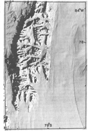
Fig.1. Landsat image of Ellsworth Mountains and Rutford Ice Stream, which flows in a southerly direction.
2 Topography
Optical levelling was carried out in 1978–79 along the longitudinal and both transverse lines. Three shorter lines were levelled in 1979–80. Results are shown in Figure 2, where contours outside the surveyed area have been extrapolated by subjective interpretation of features on Landsat images.
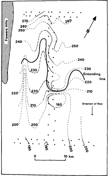
Fig.2. Surface elevation contours (m). Solid line is where the profile was optically levelled in 1978–79 and the dashed line is the area levelled in 1979–80. Pecked line is where features in Landsat images have been interpreted.
Ice thicknesses from both ground and airborne radio echo-sounding are shown in Figure 3. The contours indicate that the predominant structure is one of thick fingers of ice running parallel to the flow. The position uncertainty of the airborne results compared with the ground-based observations means that the overall accuracy is around ±20 m where contours cross sounding lines.
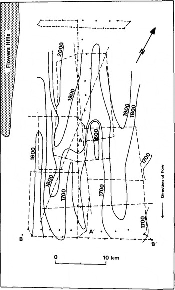
Fig.3. Ice thickness contours using data from ground based radio echo-soundings in 1978–79 and 1979–80 and airborne sounding in 1981. Dashed lines are sounding tracks. AA' and BB' are the lines of the profiles in Figure 4.
Profiles of surface and bottom elevations of the lower part of the longitudinal line and the southern transverse line are shown in Figure 4. For the transverse profile, the way in which the surface elevation increases as the ice thickens suggests that the glacier is floating in hydrostatic equilibrium. This is confirmed by plotting the variation in surface elevation against the variation in thickness, which yields a straight line. By assuming an exponential type of variation of density with depth, results from density profiles measured down to 10 m allow the average ice-column density, and hence the elevation above sea-level, to be calculated. Thus, surface elevations are known to ±5 m a.s.l. and to ±0.5 m relative to each other along the optically levelled lines.

Applying to the longitudinal profile the average Ice density calculated for the transverse profile, bottom elevations were calculated for measured surface elevations on the assumption that the ice was in hydrostatic equilibrium. As can be seen from Figure 4, while going up-stream the calculated bottom elevations agree closely with the measured bottom elevations until there is a marked divergence near the base of a prominent knoll. At this point the ice is grounded and no longer in hydrostatic equilibrium. The smaller divergence just down-stream from the knoll suggests that the glacier is depressed below its equilibrium surface elevation for about 5 km after it starts to float. Allowing for errors in surface elevations and ice thickness, the position of the grounding line is believed to be within about ±2 km.
In an attempt to define the position of the grounding line more closely, hydrostatic tiltmeters were used to measure tidal bending (Reference Stephenson, Doake and HorsfallStephenson and others 1979). Figure 5 shows the sites where tiltmeters were used on the longitudinal stake line close to the surface knoll. In the first year, only one tiltmeter was used and was aligned along the flow direction. The site at stake 19 and a site 4 km upstream showed no sign of tidal bending, whereas all six sites further down-stream (one only 600 m from stake 19) showed tidal cycles. In the second season, two tiltmeters were used as an orthogonal system to measure simultaneously bending in two directions. This time, the tiltmeters at stake 19 (now about 400 m down-stream from its position during the previous year) measured tidal bending, but only on one of the two arms. Although this time all the other sites in Figure 4 also showed bending, only those down-stream of stake 19 gave large amplitudes while those up-stream gave weak signals. At nearly all sites, bending amplitudes measured on orthogonal arms were different, sometimes markedly so. Stake 19 was near the top of the prominent knoll, so it can be seen from Figures 4 and 5 that sites up-stream from stake 19 are unequivocally on grounded ice. However, weak flexure could be expected if the grounding line passed close enough for bending stresses to be transmitted to nearby grounded sites. It is reasonable to suppose that the stresses at the grounding line would decay over distances of the order of the ice thickness, which is all that is required to explain the tiltmeter results.
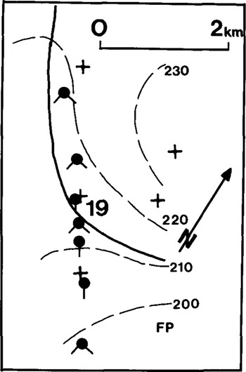
Fig.5. Sites where tiltmeters were used are shown as filled circles with the tails indicating the orientation of the tiltmeters. FP indicates one site where radio echo-fading patterns were obtained; the other site was further downstream. Crosses mark stakes, with their identification number. The thick line is the assumed grounding line and dotted lines are surface elevation contours.
By comparing measured bottom and surface elevations with those expected if the glacier was floating in hydrostatic equilibrium on the sea, maps of surface elevation and ice thickness were also used to estimate the position of the grounding line in regions away from the stake network. However, subjective extrapolation of the surface contours is uncertain, so the delineation of the grounding line away from the centre of Figure 2 should be treated with caution.
3 Movement
A complete triangulation survey of the 68 stations was carried out twice in the first season and once in 1979–80. Results from these surveys were used to produce coordinates and velocities reduced to an epoch date by the method described by Reference Wager, Doake, Paren and WaltonWager and others (1980). The velocities of three stations along the longitudinal axis were measured by a semigraphlc resection technique (Reference WaltonWalton 1979). One of these stations was used as control for the rest of the system, while the other two values were used as Independent checks on the main results. Velocities are known for all stations to within ±3%. Strainrates were computed for the centroids of triangles formed by sets of stakes along the lines and are within about ±10% (Fig.6). At two sites, a radio echo technique of comparing echo-fading patterns (Reference DoakeDoake 1975) was used to estimate the sliding velocity of the glacier.
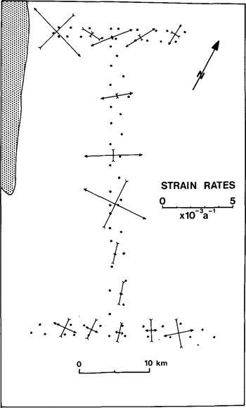
Fig.6. Strain-rates: ![]()
Figure 7 shows the longitudinal and transverse velocity profiles. The longitudinal velocity shows a steady decrease with distance down-stream; the compressive flow evidently explains the lack of surface crevassing in the hinge zone. The northern transverse velocity profile was entirely on the central part of the ice stream, while the southern profile encroached into the crevassed area of the right bank. There is a marked asymmetry in the southern velocity profile, probably caused by different conditions at the sides of the glacier. A large mass of 1ce flows into Rutford Ice Stream south of Flowers Hills, whereas the western margin of Rutford Ice Stream, further north, and the eastern margin, are all bounded by relatively thin and static ice. Figure 7 also shows a theoretical velocity profile, calculated using the equation (Reference BuddBudd 1966)
where u(o) is the centre velocity, y the distance across the glacier, and k a constant, which depends on constants in the flow law of ice, the width of the glacier, and the shear stress at the sides. The value of n, one of the flow-law constants, has been assumed to be 3. The equation was derived on the assumption that deformation occurs by simple shear at the glacier sides and is directly analogous with vertical profiles of velocity. It appears that only on the south-west arm of the profiles does the theoretical curve give a reasonable fit to the measured data. On the other arms of the profiles, deformation seems to be concentrated into a narrower boundary layer.
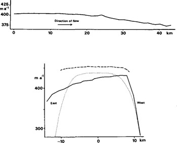
Fig.7. Surface velocity profiles: (a) longitudinal profile, (b) transverse profile. The dotted line is a theoretical profile assuming simple shear at the side walls. Dashed line is the northern profile, solid line the southern one.
The pattern of strain-rates near the margins shown in Figure 6, and revealed by the orientation of crevasses, is that expected where there is overall longitudinal compression with shear at the boundaries (Reference NyeNye 1952). There is a more complicated strain-rate pattern near the centre of the stake scheme where the knoll disturbs the flow.
Both of the sites, where radio echo-fading patterns were studied, were on floating ice (Fig.5), and showed that, within the experimental error, all forward motion was by sliding, with no discernible deformation between top and bottom surfaces of the glacier.
4 Discussion
The longitudinal velocity and thickness profiles down-stream from the grounding line were modelled using a modified version of the method described by Reference SandersonSanderson (1979) for finding equilibrium profiles of ice shelves. The same method has been used by Reference Crabtree and DoakeCrabtree and Doake (1982) for modelling Pine Island Glacier. The principle of continuity of mass is used in the form
where a is the net accumulation of top and bottom surfaces, u the horizontal velocity, ![]() the thickness, gradient in the flow direction, h the ice thickness, and
the thickness, gradient in the flow direction, h the ice thickness, and ![]() the vertical strain-rate (positive for extending). Rewriting Equation (1) in the form
the vertical strain-rate (positive for extending). Rewriting Equation (1) in the form
shows that if the parameters on the right-hand side are known, or can be calculated, then a thickness profile can be constructed. The longitudinal strain rate ![]() can be expressed as
can be expressed as
where ρe is a density parameter which takes into account the restraining effect of sea-water pressure, g the acceleration due to gravity, n and B̅ constants in the flow law for ice when expressed in the form ![]() , and Fr is the total force per unit width restraining movement by shear at the side walls or by pinning on ice rises or shoals. The velocity profile is given simply by
, and Fr is the total force per unit width restraining movement by shear at the side walls or by pinning on ice rises or shoals. The velocity profile is given simply by
where u(o) is the velocity at the grounding line. Good agreement with the measured profiles was obtained by using the values of the parameters given in Table I. The Rutford profiles can best be matched by assuming a constant restraining force Fr and zero shear stress at the margins. However, the section is too short (15 km) to be able to attach too much significance to this result. The surface accumulation rate was determined from two oxygen isotope profiles to 10 m depth to be 0.30 Mg m−2 a−1 ; combining this figure with that of the net accumulation from Table I implies a bottom melt rate of 1.7 Mg m−2 a−1. It appears from Figure 1 that the sides of Rutford Ice Stream diverge in the direction of flow at about 6°. Using measured values of flow velocity and ice-stream width this would imply a lateral strain-rate of around 3 × 10⁻³ a−1. This is the value measured over the grounded ice, but lateral strain-rates along the centre line of the floating ice were found to be an order of magnitude less. Evidently the ice flowing into Rutford Ice Stream south of Flowers Hills is constraining the lateral flow. The measured lateral strain-rates were used in the model.
Conclusion
The grounding-line area of Rutford Ice Stream has a complex morphology. Tidal flexure can be measured over large areas and probably even where ice is aground. Transverse velocity profiles show that most of the ice deformation is concentrated at the sides, implying that the side-wall shear stress plays a less important role in determining the overall motion of the ice stream than does the Ronne Ice Shelf into which the ice stream flows. The ice stream consists of several thick ice tongues running along the flow direction and separated by thinner narrow troughs. Slopes of both ice surface and bedrock are small in the direction of flow. The overall surface gradient as is about 1.8 × 10⁻³, which implies that groundingline migration velocities Vm in response to changes in ice thickness ![]() could be very large: approximate values can be found from the equation of Reference Thomas and BentleyThomas and Bentley (1978), written in the form
could be very large: approximate values can be found from the equation of Reference Thomas and BentleyThomas and Bentley (1978), written in the form
showing that ice thinning of 0.5 m a−1 would give Vm as 250 m a−1. Continued monitoring of the grounding line should indicate, in a few years, whether or not there is any change in position.
Table 1. VALUES OF PARAMETERS USED IN MODEL

Acknowledgements
The field assistance of J L W Walton, R V Otto, H E Thompson, and R Airey is gratefully acknowledged. Walton and Otto also reduced the survey data.


