


1. Introduction
In recent years there has been a resurgence in low-frequency radio astronomy. LOFAR (van Haarlem et al. Reference van Haarlem2013) and the Murchison Widefield Array (Tingay et al. Reference Tingay2013) in particular have proven to be excellent tools for probing of the ionosphere. In a series of papers, Loi et al. (Reference Loi2015a,b,c, Reference Loi2016a,b) demonstrated the capability of the Murchison Widefield Array to measure exquisitely the 2D spatial derivatives of the Total Electron Content (TEC) of the ionosphere via measurements of the refractive shifts of the several hundred sources visible in a typical MWA snapshot image. A wide range of phenomena were observed, including Travelling Ionospheric Disturbances (TIDs) and magnetic field aligned structures which were shown (via parallax imaging) to be located in the magnetosphere. This method of refractive shift measurement, and statistics derived from it has become the de facto metric by which ionospheric activity is measured in MWA observations (Jordan et al. Reference Jordan2017). They have been studied extensively (Helmboldt & Hurley-Walker Reference Helmboldt and Hurley-Walker2020), and methods have also been developed to mitigate the effects of refractive distortion for imaging (Hurley-Walker & Hancock Reference Hurley-Walker and Hancock2018) and source astrometry (Morgan et al. Reference Morgan2018).
Meanwhile, Mevius et al. (Reference Mevius2016) have used LOFAR to measure the ionosphere using phase calibration solutions. This results in a measurement of phase variance per baseline length, allowing the structure function (see Section 4.2) of the ionosphere to be constructed for baselines from 0.1 to 100 km. A similar approach has been used by Rioja & Dodson (Reference Rioja and Dodson2022), to use the long-baseline configuration of Phase-II MWA (Wayth et al. Reference Wayth2018; Beardsley et al. Reference Beardsley2019) to probe the ionosphere down to scales of around 600 m.
Although both methods are extremely sensitive to very small gradients in the electron density, they are both most sensitive to structures larger than ${\sim}$
1 km. Since refractive shifts are measured in the image plane, they are averaged over all baselines, which for most visibility weighing schemes leads to an average baseline length
${\sim}$
1 km. Since refractive shifts are measured in the image plane, they are averaged over all baselines, which for most visibility weighing schemes leads to an average baseline length ${>}1\,\textrm{km}$
for the MWA. For measurements based on phase calibration solutions, the relatively small phase variations due the ionosphere on shorter baseline lengths are small compared with in phase variance due to thermal noise for baselines shorter than a few hundred metres (see e.g. Figure 3 of Mevius et al. Reference Mevius2016). The smallest ionospheric structure may also be undetectable to both methods if the data are integrated too much in time, since even with very low drift velocities of
${>}1\,\textrm{km}$
for the MWA. For measurements based on phase calibration solutions, the relatively small phase variations due the ionosphere on shorter baseline lengths are small compared with in phase variance due to thermal noise for baselines shorter than a few hundred metres (see e.g. Figure 3 of Mevius et al. Reference Mevius2016). The smallest ionospheric structure may also be undetectable to both methods if the data are integrated too much in time, since even with very low drift velocities of ${\sim}10\,\mathrm{m s}^{-1}$
(e.g. Asaki et al. Reference Asaki2007) smaller structures will drift over the array in less than a minute.
${\sim}10\,\mathrm{m s}^{-1}$
(e.g. Asaki et al. Reference Asaki2007) smaller structures will drift over the array in less than a minute.
The fact that the ionosphere at the small, ${\sim}$
300 m scales remains unexplored with the MWA motivated us to investigate the use of ionospheric scintillation to probe these scales. The effects of ionospheric scintillation on Global Navigation Satellite Systems (GNSS) is well-known, and is a widely-used probe of the ionosphere (Kintner, Ledvina, & de Paula Reference Kintner, Ledvina and de Paula2007) in the more extreme ionospheric conditions found in the polar (Spogli et al. Reference Spogli2009) and equatorial regions (Beach et al. Reference Beach, Kelley, Kintner and Miller1997). Scintillation increases with observing wavelength. Therefore, at MWA and LOFAR frequencies, an order of magnitude lower than those used for GNSS, we would expect scintillation to be measurable even for the benign mid-latitude ionosphere observable where these telescopes are (by design) located.
${\sim}$
300 m scales remains unexplored with the MWA motivated us to investigate the use of ionospheric scintillation to probe these scales. The effects of ionospheric scintillation on Global Navigation Satellite Systems (GNSS) is well-known, and is a widely-used probe of the ionosphere (Kintner, Ledvina, & de Paula Reference Kintner, Ledvina and de Paula2007) in the more extreme ionospheric conditions found in the polar (Spogli et al. Reference Spogli2009) and equatorial regions (Beach et al. Reference Beach, Kelley, Kintner and Miller1997). Scintillation increases with observing wavelength. Therefore, at MWA and LOFAR frequencies, an order of magnitude lower than those used for GNSS, we would expect scintillation to be measurable even for the benign mid-latitude ionosphere observable where these telescopes are (by design) located.
Depending on the observing parameters, scattering effects can manifest in different ways, including amplitude scintillation as well as rapid image-plane distortion. This is illustrated in Figure 1. This figure shows that if we assume that the diffractive scales ( $r_\textrm{diff}$
) measured by Jordan et al. (Reference Jordan2017) and Mevius et al. (Reference Mevius2016) apply on the smaller scales probed by scintillation, we would expect to be firmly in the ‘weak amplitude scintillation’ regime. In this weak scatter regime, the scattering strength corresponds to the scintillation index, so we would expect indices of a few percent.Footnote a This is confirmed in real data from the MWA, where temporal power spectra of bright sources observed with the MWA clearly show amplitude scintillation of a few percent (Morgan & Ekers Reference Morgan and Ekers2021). Dynamic spectra of a scintillating source observed by LOFAR at observing frequencies of 10–80 MHz by Fallows et al. (Reference Fallows2020) are also consistent with this picture, with weak amplitude scintillation in the upper half of the band, and strong amplitude scintillation (characterised by spectral structure) evident at the lowest frequencies.
$r_\textrm{diff}$
) measured by Jordan et al. (Reference Jordan2017) and Mevius et al. (Reference Mevius2016) apply on the smaller scales probed by scintillation, we would expect to be firmly in the ‘weak amplitude scintillation’ regime. In this weak scatter regime, the scattering strength corresponds to the scintillation index, so we would expect indices of a few percent.Footnote a This is confirmed in real data from the MWA, where temporal power spectra of bright sources observed with the MWA clearly show amplitude scintillation of a few percent (Morgan & Ekers Reference Morgan and Ekers2021). Dynamic spectra of a scintillating source observed by LOFAR at observing frequencies of 10–80 MHz by Fallows et al. (Reference Fallows2020) are also consistent with this picture, with weak amplitude scintillation in the upper half of the band, and strong amplitude scintillation (characterised by spectral structure) evident at the lowest frequencies.
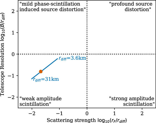
Figure 1. Scattering strength vs baseline length in terms of scattering scale, following Cornwell et al. (Reference Cornwell, Anantharamaiah and Narayan1989). Descriptions of asymptotic regimes are also from Cornwell et al. (though we adopt our definition of $r_F$
; see Equation (7)). The blue line is for the range of
$r_F$
; see Equation (7)). The blue line is for the range of $r_\mathrm{diff}$
observed by Mevius et al. (Reference Mevius2016), but scaled to our observing frequency of 154 MHz. Baseline length B is assumed to be 2.2 km (MWA Phase I). The orange point is calculated from the scintillation index observed by Morgan & Ekers (Reference Morgan and Ekers2021) with the MWA at 162 MHz. Height of the ionosphere is assumed to be 300 km.
$r_\mathrm{diff}$
observed by Mevius et al. (Reference Mevius2016), but scaled to our observing frequency of 154 MHz. Baseline length B is assumed to be 2.2 km (MWA Phase I). The orange point is calculated from the scintillation index observed by Morgan & Ekers (Reference Morgan and Ekers2021) with the MWA at 162 MHz. Height of the ionosphere is assumed to be 300 km.
Weak scintillation measurements are sensitive to structures close to the Fresnel Scale $r_{\text{F}}$
(defined in Equation (7)), around 300 m at MWA frequencies and typical ionospheric heights, thus allowing us to probe spatial scales an order of magnitude smaller than those probed by refractive shifts, and even smaller than the scales probed by Rioja & Dodson (Reference Rioja and Dodson2022).
$r_{\text{F}}$
(defined in Equation (7)), around 300 m at MWA frequencies and typical ionospheric heights, thus allowing us to probe spatial scales an order of magnitude smaller than those probed by refractive shifts, and even smaller than the scales probed by Rioja & Dodson (Reference Rioja and Dodson2022).
Beyond the opportunity to explore new parameter space, amplitude scintillation is also interesting in that it may be measured with much more modest instruments than LOFAR or the MWA, since it does not require baselines longer than 100 m.
Below, we present amplitude scintillation measurements from several thousand MWA Epoch of Reionisation observations (Trott et al. Reference Trott2020). Importantly, the ionosphere has already been characterised via refractive shifts for all of these observations, permitting a comparison of these two observables.
The paper is organised as follows: in Section 2 we describe our observations and the refractive shift analysis that has already been completed. In Section 3 we describe our methodology for measuring ionospheric scintillation. In Section 4 we present our results and in Section 5 we give our conclusions and offer our suggestions for future work.
2. Observations
As an extension of the work in Jordan et al. (Reference Jordan2017), more EoR observations were calibrated and analysed for their ionospheric activity. While the results of this work have not been published in their own right, they have still contributed to other projects, such as that presented in Trott et al. (Reference Trott2020).
In total the ionospheric refractive shift analysis has been carried out on $29070 \times 2-\textrm{min}$
observations across 350 nights. These nights include data from the ‘EoR-0’, ‘EoR-1’ and ‘EoR-2’ MWA fields. All observations were taken between August 2013 and January 2016 in the MWA Phase I configuration, and were conducted in the ‘drift-and-shift’ strategy where the pointing centre is periodically updated to keep the target EoR field close to the centre of the primary beam. They utilise the full 30.72 MHz of MWA instantaneous bandwidth in one contiguous block at one of two centre frequencies: 182 MHz (EoR ‘high-band’: 10777 observations) or 154 MHz (EoR ‘low-band’: 15425 observations).
$29070 \times 2-\textrm{min}$
observations across 350 nights. These nights include data from the ‘EoR-0’, ‘EoR-1’ and ‘EoR-2’ MWA fields. All observations were taken between August 2013 and January 2016 in the MWA Phase I configuration, and were conducted in the ‘drift-and-shift’ strategy where the pointing centre is periodically updated to keep the target EoR field close to the centre of the primary beam. They utilise the full 30.72 MHz of MWA instantaneous bandwidth in one contiguous block at one of two centre frequencies: 182 MHz (EoR ‘high-band’: 10777 observations) or 154 MHz (EoR ‘low-band’: 15425 observations).
For this work we restricted ourselves to Low-band EoR-0 observations: which covers 5251 observations in total. However, visibility data for some of these observations are no longer available (typically ones observed further from the zenith). We also restricted ourselves to observations taken in 2014, and rejected those with 8 or more tiles flagged. This left us with 2070 observations for further analysis.
2.1 Refractive shift analysis
As with Jordan et al. (Reference Jordan2017), these 29070 observations have had their ionospheric activity categorised into ‘magnitude’ and ‘anisotropy’ components. The ‘magnitude’ corresponds to the median observed ionospheric refractive shift, after they have been normalised to 200 MHz (ionospheric shifts scale with the square of wavelength), and the ‘anisotropy’ is determined by a Principal Component Analysis (PCA). The ionospheric shifts are two-dimensional (typically in Right Ascension and Declination) and so a PCA yields two eigenvalues; if the eigenvalues are the same, the data is purely anisotropic. On the other hand, if there is even a slight trend for ionospheric shifts lie along an axis, one eigenvalue will be larger the other; it is the dominant eigenvalue that is recorded for categorisation, normalised such that the sum of the eigenvalues is unity (i.e. the anisotropy values all lie in the range 0.5–1.0).
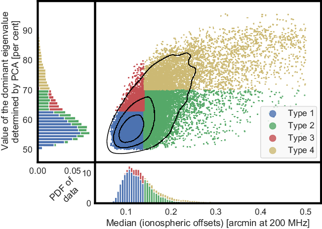
Figure 2. A scatter plot of the median ionospheric offset versus the anisotropy, which is the dominant eigenvalue determined by PCA for all 29070 EoR MWA observations. The 4 distinct ionospheric populations, or ‘types’, are also included.
Using the ionospheric data collected from each observation, Jordan et al. (Reference Jordan2017) categorised four populations of ionospheric activity, as shown on Figure 2. These classifications were labelled as Types 1 through 4, all of which have been specifically identified using the following criteria:
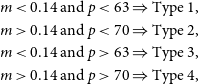 \begin{align*} m & < 0.14 \text{ and } p < 63 \Rightarrow \text{Type 1,}\\m & > 0.14 \text{ and } p < 70 \Rightarrow \text{Type 2,}\\ m & < 0.14 \text{ and } p > 63 \Rightarrow \text{Type 3,}\\ m & > 0.14 \text{ and } p > 70 \Rightarrow \text{Type 4,}\end{align*}
where m is the median ionospheric offset and p is the dominant eigenvalue in per cent. This categorisation has divided the total 2070 observations in this analysis into approximately 70, 6, 13 and 11 per cent for ionospheric Types 1 through 4, respectively.
2.2 IPS sources in the EOR-0 field
Interplanetary Scintillation (IPS) causes compact (sub-arcsecond) sources to vary in brightness on ${\sim}$
1 s timescales. IPS on the nightside is weaker than it is closer to the Sun; nonetheless scintillation indices can be as high as 5% under typical conditions (Bell Reference Bell1968), and may occasionally be much higher (Kaplan et al. Reference Kaplan2015). Although somewhat separable from ionospheric scintillation due to its shorter timescale, IPS is nonetheless an important potential contaminant. However, in contrast to ionospheric scintillation, which will affect all discrete sources in the EoR field, only the very compact components of sources will show IPS. We therefore utilised as-yet unpublished MWA IPS observations covering the EoR-0 field from the MWA IPS Survey (Morgan et al. Reference Morgan2019) to determine the extent to which each source in the field might be affected by IPS. Restricting ourselves to the brightest sources (White et al. Reference White2020), for each we calculated the Normalised Scintillation Index (NSI; Chhetri et al. Reference Chhetri2018): the ratio of the observed scintillation index to that expected for a point source.
${\sim}$
1 s timescales. IPS on the nightside is weaker than it is closer to the Sun; nonetheless scintillation indices can be as high as 5% under typical conditions (Bell Reference Bell1968), and may occasionally be much higher (Kaplan et al. Reference Kaplan2015). Although somewhat separable from ionospheric scintillation due to its shorter timescale, IPS is nonetheless an important potential contaminant. However, in contrast to ionospheric scintillation, which will affect all discrete sources in the EoR field, only the very compact components of sources will show IPS. We therefore utilised as-yet unpublished MWA IPS observations covering the EoR-0 field from the MWA IPS Survey (Morgan et al. Reference Morgan2019) to determine the extent to which each source in the field might be affected by IPS. Restricting ourselves to the brightest sources (White et al. Reference White2020), for each we calculated the Normalised Scintillation Index (NSI; Chhetri et al. Reference Chhetri2018): the ratio of the observed scintillation index to that expected for a point source.
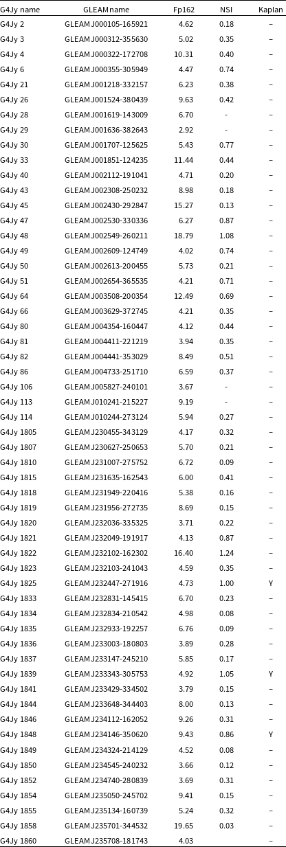
These NSIs are listed in Table 1. Errors are approximately 20% (note also that since the IPS observations were made when the Sun was active, it is possible that some of these NSIs are overestimated). By selecting only NSI $<0.2$
sources and filtering out IPS timescales (see Section 3.3), we reduce IPS variability to well below 1%.
$<0.2$
sources and filtering out IPS timescales (see Section 3.3), we reduce IPS variability to well below 1%.
Table 1. IPS Normalised Scintillation indices of G4JY sources within 15 degrees of the centre of the EoR-0 field. ‘Fp162’ is the GLEAM (Hurley-Walker et al. Reference Hurley-Walker2017) flux density at the IPS observing frequency. NSI is the normalised scintillation index as defined by Chhetri et al. (Reference Chhetri2018). ‘Kaplan’ indicates the three sources detected by Kaplan et al. (Reference Kaplan2015).
3. Method
3.1 Calibration
First, a calibration solution was produced for each observation (Offringa et al. Reference Offringa2015) using a sky model (Hurley-Walker et al. Reference Hurley-Walker2017) attenuated by the primary beam. A single calibration solution was produced using the full two-minute observation. In addition to this, purely for quality control purposes, we found it useful to generate a calibration solution for each individual 2-s correlator integration time. Examination of the phase as a function of time using these calibration solutions allowed us to identify phase jumps due to instrumental issues, which affected a small subset of observations.
3.2 Imaging
By applying the calibration solutions and using WSClean (Offringa et al. Reference Offringa2014), a ‘standard image’ was created for each observation using the whole 2 min of observing time, and all unflagged tiles of the full Phase I MWA. This image was deconvolved using image-based CLEAN interspersed with up to 5 ‘major cycles’, where the CLEAN components were subtracted from the visibilities. The final ‘model’ visibilities, comprising all the CLEAN components, was written to the visibility measurement set for later use. A final standard image, as shown on the left in Figure 3, was created by combining the individual synthesis images of both linear polarisations XX and YY with appropriate weightings (Sault, Staveley-Smith, & Brouw Reference Sault, Staveley-Smith and Brouw1996, Equation (1)).
Next, ‘snapshot’ images were generated for each individual 2-s time integration for each polarisation (excluding the first 2 and last 3 integrations, resulting in 51 snapshots per observation). These differed from the standard images significantly in two ways: first, the model derived from the standard image deconvolution process was subtracted from the visibilities, leaving only the residuals to be imaged. Second, any tiles from beyond the central 100-m ‘core’ of the MWA were flagged, reducing the number of tiles to 36 and decreasing the average baseline length to smaller than the Fresnel scale ( $r_{\text{F}}\sim$
300 m), whereas the resolution of the snapshot images (
$r_{\text{F}}\sim$
300 m), whereas the resolution of the snapshot images ( $1.38^\circ\times1.06^\circ$
) corresponds to an average baseline length
$1.38^\circ\times1.06^\circ$
) corresponds to an average baseline length ${\sim}$
100 m.
${\sim}$
100 m.
The snapshot images were then stored using the image cube format described by Morgan et al. (Reference Morgan2018) Appendix I. This image format allows for the examination of the time series corresponding to any pixel, as well as facilitating the other timeseries analyses described below.
Figure 4 shows timeseries for the brightest sources in the field of view for observations representative of both ‘high’ and ‘low’ ionospheric scintillation. Variability on timescales consistent with ionospheric scintillation (which is clearly resolved with time resolution of 2 s) is clearly visible, as is IPS for those sources with NSI ${>}0.2$
. Note that the timeseries have a non-zero mean offset. This may be due to the presence of extended structure in the field (Lenc et al. Reference Lenc2017) which will not be included in the subtracted model. The observation length is relatively short compared to the scintillation timescale, so averaging over sources and/or observations will be necessary in order to avoid sampling errors.
${>}0.2$
. Note that the timeseries have a non-zero mean offset. This may be due to the presence of extended structure in the field (Lenc et al. Reference Lenc2017) which will not be included in the subtracted model. The observation length is relatively short compared to the scintillation timescale, so averaging over sources and/or observations will be necessary in order to avoid sampling errors.
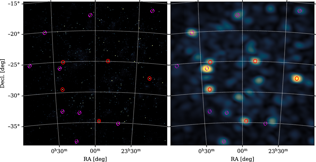
Figure 3. Standard image (left) and variability image (right) of the centre of the EoR-0 field for a strong scintillation observation (18.1%). Indicated are the top 15 brightest sources that are catalogued in the GLEAM 4Jy sample (White et al. Reference White2020), with the high-NSI sources (magenta) distinguished from the 5 low-NSI sources (red) which are the ones used to calculate the scintillation index for an observation.
Figure 5 shows power spectra for a specific source in high, medium and weak scintillation observations. The power spectrum shows a shape characteristic of scintillation, with high low-frequency power and the Fresnel ‘Knee’ marking the onset of a power law drop-off down to the noise level.
3.3 Scintillation analysis
Following Morgan et al. (Reference Morgan2018), it is possible to create an image of the variability in the field of view by taking the standard deviation of the flux density time series after filtering the timeseries to emphasise timescales of interest. This consisted of applying a low-pass Butterworth filter (order 2) with a cutoff frequency of 0.125 Hz to attenuate IPS variability. This ‘variability’ image, as seen on the right of Figure 3, is a summary of the time series as it collapses the time dimension of the previously created three-dimensional image cube. All pixels will have positive values (which are non-zero due to thermal noise). Any pixel corresponding to a source undergoing amplitude scintillation will have excess variance, and it is possible to identify sources with significant excess variability as
 \begin{equation} P - \mu > 5\sigma,\end{equation}
where P is the pixel value, $\mu$
is the background level, and
$\mu$
is the background level, and $\sigma$
is the spatial rms of the image. Identification of varying sources is therefore very similar to the problem of identifying discrete sources in any astrophysical image.
$\sigma$
is the spatial rms of the image. Identification of varying sources is therefore very similar to the problem of identifying discrete sources in any astrophysical image.
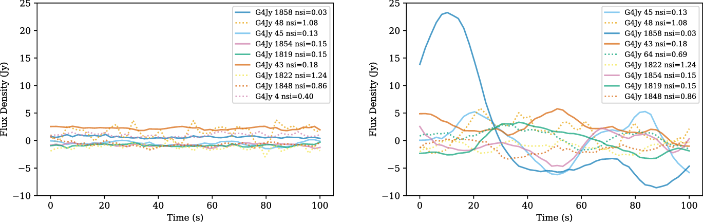
Figure 4. Time series analysis for low- (left, 1.2%) and a high- (right, 24.8%) scintillation observation, both at a frequency of 154 MHz, with off-source noise included. Sources with an NSI of above 0.2 are classified as high-NSI, or strong-IPS sources and are shown as dotted lines. These sources will follow variability on IPS timescales (1–2 s), while the low-NSI, weak-IPS sources (filled line) display variation on a timescale of 10s, which is consistent with ionospheric scintillation, particularly prominent in higher scintillation observations.
After the creation of the variability images, Aegean (Hancock et al. Reference Hancock, Murphy, Gaensler, Hopkins and Curran2012) was used to identify sources in the standard image. Once the sources were identified, they were cross-matched with the GLEAM 4Jy sample (White et al. Reference White2020): a subset of the MWA GLEAM survey (Hurley-Walker et al. Reference Hurley-Walker2017). The brightest non-IPS sources (NSI $<$
0.2) were then identified (usually the 5 ‘Low-NSI’ sources shown in Figure 3). The pixel in the moment image closest to the continuum detection was measured as well as four off-source pixels (25 pixels away) surrounding the detection.
$<$
0.2) were then identified (usually the 5 ‘Low-NSI’ sources shown in Figure 3). The pixel in the moment image closest to the continuum detection was measured as well as four off-source pixels (25 pixels away) surrounding the detection.
It is then possible to calculate the scintillation index m of each source
 \begin{equation} m = \frac{\Delta S}{S_{\text{standard}}},\end{equation}
where $S_\mathrm{standard}$
is the brightness of the given source as is found in the standard image and
$S_\mathrm{standard}$
is the brightness of the given source as is found in the standard image and $\Delta S$
is the excess variability of the source. Since the variability image values are standard deviations (i.e. the square root of the variance), the noise must be subtracted in quadrature. Therefore,
$\Delta S$
is the excess variability of the source. Since the variability image values are standard deviations (i.e. the square root of the variance), the noise must be subtracted in quadrature. Therefore,
 \begin{equation} \Delta S^2 = P^2 - \mu^2,\end{equation}
where P and $\mu$
are as defined in Equation (1).
$\mu$
are as defined in Equation (1).
The median scintillation index across all sources was then computed for each observation, reducing the scintillation level of each observation down to a single number which can be compared with metrics derived from refractive shifts.
4. Results
The left panel of Figure 6 compares the calculated scintillation index and the positional refractive shifts for all observations analysed. There is clearly a strong, positive correlation between the two metrics (Pearson correlation coefficient 0.71). However, the correlation breaks down for some observations. In particular there is a small subset of observations with a much higher refractive shift/lower scintillation index than the general trend. All of these outliers belong to two nights, as indicated in Figure 6. These two nights are discussed further in Section 4.1 below.
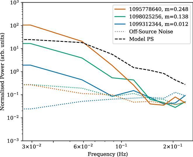
Figure 5. Power spectrum analysis for a bright, low-NSI source, G4Jy 45 (GLEAM J002430-292847) for a high (24.8%), mid (13.8%), and low (1.2%) scintillation observation, with the off-source noise power spectra included. The presence of the ‘Fresnel knee’ at the corresponding frequency assures ionospheric scintillation is being analysed, and each observation drops off to the background noise level at higher frequencies. Included in the figure is a model power spectrum weak scintillation theory (Macquart & de Bruyn Reference Macquart and de Bruyn2007), with a height to the ionosphere taken as 300 km (Hunsucker & Hargreaves Reference Hunsucker and Hargreaves2002; Wild & Roberts Reference Wild and Roberts1956), and a velocity of 50 m s-1 (Asaki et al. Reference Asaki2007).
There is also a less extreme set of observations where the observed scintillation index is higher than the trend. The refractive shift of these sources spans all but the very lowest refractive shift.
The existence of any correlation between the anisotropy metric, either positive or negative, is far less clear: the apparent correlation between scintillation index and anisotropy in the right panel of Figure 6 (see also Figure 8 which shows the anisotropy as a colour bar) appears to be driven more by the correlation between refractive shift and anisotropy.
4.1 Discrepant nights
As already noted, almost all the most discrepant points in the plot of refractive shift vs scintillation index belong to two specific nights: 2014 September 26 and 2014 November 24. On both these nights, a handful of observations were classified as Type II’s, although they are all very close to the Type II/Type IV boundary, indicating the presence of higher levels of structure.
On both of these nights a Travelling Ionospheric Disturbance (TID) traverses the field, with an exceptionally active one on 2014 September 26, leading to much higher scintillation indices in parts of the field. As is shown on the leftmost top plot in Figure 7, earlier in the TID’s path it is directly passing over and affecting the sources that were sampled for the scintillation analysis, but as it moves north, shown on the rightmost top plot in Figure 7, the sources that were being monitored go back to lower levels of scintillation, whereas due to larger sampling used, the TID was still being captured by the shift metric. Thus, the apparent discrepancy between the two metrics on 2014 September 26 is due to sampling differences.
In contrast, the location of the TID that was captured by observations from 2014 November 24 (lower panels of Figure 7), is well-sampled by the scintillating sources, even where the observations are maximally discrepant as those shown in Figure 6. The night of this TID event can be separated into three clusters, each occupying a different space within Figure 8. Before the TID enters the field, both metrics indicate low ionospheric activity. Then the refractive shifts increase, then the ionospheric scintillation increases as the refractive shifts decrease. This is indicated in Figure 8, where the arrows between the clusters indicate the progression of time.
4.2 Relating refractive shift and scintillation index with power law turbulence
In turbulent scattering media, the phase structure function takes the form of a power law (Rino Reference Rino1979)
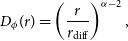 \begin{equation} D_{\phi}(r) = \left(\frac{r}{r_{\text{diff}}}\right)^{\alpha-2},\end{equation}
where the ‘diffractive scale’, $r_{\text{diff}}$
, is the spatial scale over which the phase variance is 1
$r_{\text{diff}}$
, is the spatial scale over which the phase variance is 1 $\text{rad}^2$
and the
$\text{rad}^2$
and the $\alpha$
is the power law index: 11/3 for Kolmogorov turbulence (Narayan Reference Narayan1992). Mevius et al. (Reference Mevius2016) found values for
$\alpha$
is the power law index: 11/3 for Kolmogorov turbulence (Narayan Reference Narayan1992). Mevius et al. (Reference Mevius2016) found values for $\alpha$
in the range 11/3–12/3, and
$\alpha$
in the range 11/3–12/3, and $r_\mathrm{diff}$
in the range 3.5–31.1 km.
$r_\mathrm{diff}$
in the range 3.5–31.1 km.
The ratio of the phase structure function for different values of r is given simply by
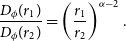 \begin{equation} \frac{D_{\phi}(r_1)}{D_{\phi}(r_2)} = \left(\frac{r_1}{r_2}\right)^{\alpha-2}.\end{equation}
Both the scintillation index and the refractive shift are measures of the structure function on different scales.
The scintillation index, m, in the weak regime measures the structure function on the Fresnel scale $r_{\text{F}}$
(Narayan Reference Narayan1992)
$r_{\text{F}}$
(Narayan Reference Narayan1992)
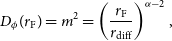 \begin{equation} D_{\phi}(r_\mathrm{F}) = m^2 = \left(\frac{r_\mathrm{F}}{r_{\text{diff}}}\right)^{\alpha-2},\end{equation}
where $r_{\text{F}}$
depends purely on the distance to the scattering screen h, and the observing wavelength
$r_{\text{F}}$
depends purely on the distance to the scattering screen h, and the observing wavelength $\lambda$
:
$\lambda$
:
 \begin{equation} r_{\text{F}} = \sqrt{\frac{\lambda h}{2\pi}} .\end{equation}
Each measurement of a refractive shift measures the spatial gradient of the phase screen. All baselines contribute to the measurement, so if we take the average baseline length, B (where B=2.2 km for our data Jordan et al. Reference Jordan2017),
 \begin{equation} D_{\phi}(B) = \left(\frac{2 \pi \theta B}{\lambda}\right)^2,\end{equation}
where $\theta$
is the refractive shift in radians. Note that we take the median shift of all the sources in the field of view: an average of a spatial ensemble of point measurements of
$\theta$
is the refractive shift in radians. Note that we take the median shift of all the sources in the field of view: an average of a spatial ensemble of point measurements of $D_{\phi}(B)$
over a region of the ionosphere
$D_{\phi}(B)$
over a region of the ionosphere ${\sim}$
100 km across (c.f. Jordan et al. Reference Jordan2017, Section 4.2.1).
${\sim}$
100 km across (c.f. Jordan et al. Reference Jordan2017, Section 4.2.1).
Figure 9 shows the expected relationship between m and $\theta$
from Equations (5), (6) and (8). Since both
$\theta$
from Equations (5), (6) and (8). Since both $\theta^2$
and
$\theta^2$
and $m^2$
measure phase variance, m and
$m^2$
measure phase variance, m and $\theta$
will be proportional to each other in the case of power law turbulence. Adjusting either the power law index of the turbulence,
$\theta$
will be proportional to each other in the case of power law turbulence. Adjusting either the power law index of the turbulence, $\alpha$
, or the distance to the scattering screen, h, will change the constant of proportionality, but h and
$\alpha$
, or the distance to the scattering screen, h, will change the constant of proportionality, but h and $\alpha$
are degenerate as far as the relationship between m and
$\alpha$
are degenerate as far as the relationship between m and $\theta$
is concerned.
$\theta$
is concerned.
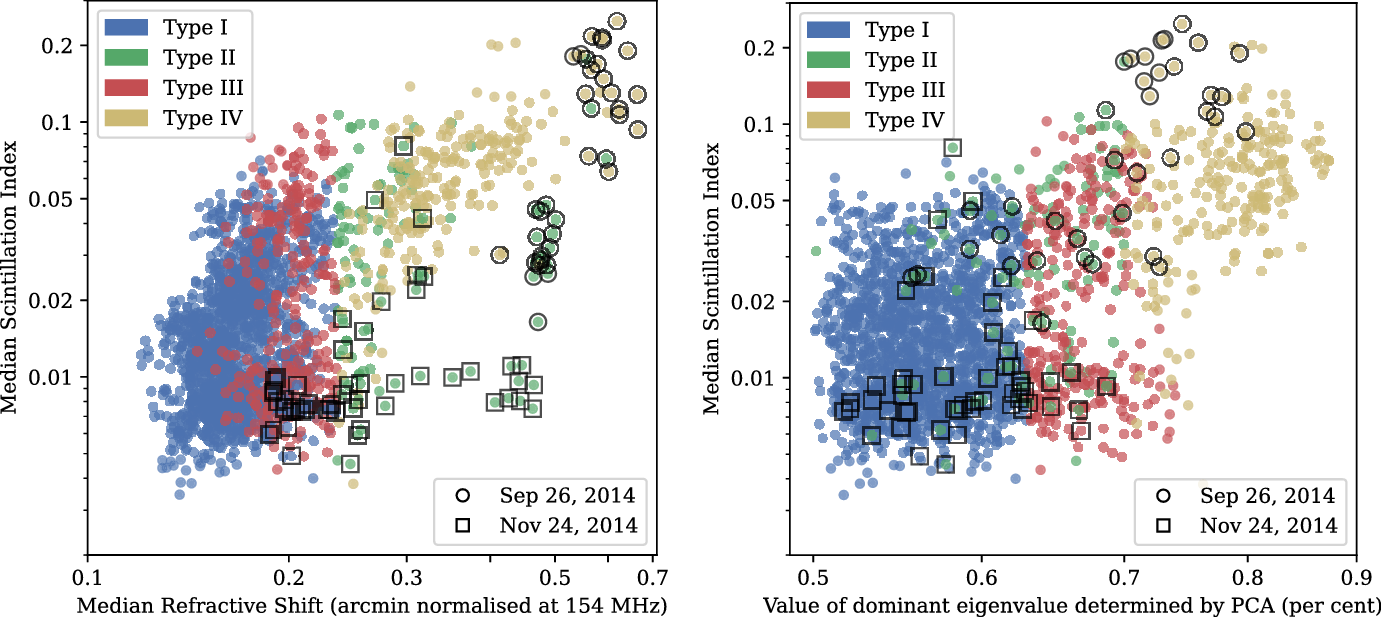
Figure 6. The median scintillation index calculated using the low-NSI sources in the MWA EoR-0 field, compared to the median refractive shift (left) and the anisotropy of an observation, a value of the dominant eigenvalue as determined by a principal component analysis (PCA) (right). The refractive shift as found by Jordan et al. (Reference Jordan2017) is calculated at a frequency of 200MHz, therefore for this comparison the refractive shifts were normalised to a frequency of 154 MHz. Highlighted in both figures are observations from two nights of particular interest; 2014 November 24 and 2014 September 26, both of which have a Travelling Ionospheric Disturbance (TID) traverse the field.
Examining our measurements relative to the theoretical relationship, we find that Kolmogorov turbulence predicts a somewhat higher scintillation index for a given refractive shift than is observed for the vast majority of observations. The expected relationship fits the data relatively well when the ionosphere is quite active; however for the majority of observations, where the ionosphere is quiet according to both metrics, the scintillation index is much lower than would be expected given the refractive shift. We note that in the absence of refractive shifts, sources will still be shifted due to noise. Since the refractive shift metric was intended only to identify observations of high ionospheric activity, no attempt was made to subtract this noise. It is also possible that non-turbulent structures, such as those discovered by Loi et al. (Reference Loi2015c) are persistent in the refractive shift data at some level. For our ionospheric scintillation measurements, the noise was subtracted (see Equation (3)), although other sources of variability, such as residual IPS, or change of instrumental response as the sky rotates may still be positively biasing the scintillation indices. Nonetheless, it is plausible that the true refractive shifts of many of the Type I observations are much lower than those presented here, and they may therefore lie closer to the expected relationship.
5. Discussion
5.1 Interpretation
We have measured ionospheric scintillation across a representative sample of $2\,070\times2$
-min MWA observations and compared them with a refractive shift analysis already carried out. The range of scintillation indices seen matches predictions reasonably well (Figure 1), and there is a correlation of 0.71 between the observed scintillation index and average refractive shift. Moreover, at least for more active ionospheres, the relationship between scintillation index and refractive shift is broadly in line with what would be expected if the ionosphere’s structure is well described by Kolmogorov turbulence between the relevant scales of
$2\,070\times2$
-min MWA observations and compared them with a refractive shift analysis already carried out. The range of scintillation indices seen matches predictions reasonably well (Figure 1), and there is a correlation of 0.71 between the observed scintillation index and average refractive shift. Moreover, at least for more active ionospheres, the relationship between scintillation index and refractive shift is broadly in line with what would be expected if the ionosphere’s structure is well described by Kolmogorov turbulence between the relevant scales of $2.2$
km down to the Fresnel scale
$2.2$
km down to the Fresnel scale ${\sim}300$
m. This is entirely consistent with previous observations, such as those of Mevius et al. (Reference Mevius2016).
${\sim}300$
m. This is entirely consistent with previous observations, such as those of Mevius et al. (Reference Mevius2016).
Power law turbulence arises naturally when energy cascades from large scales to small scales without dissipation; the spectral index of -11/7 arising from dimensional arguments (Kolmogorov Reference Kolmogorov1941). Kolmogorov turbulence is an excellent model for a broad range of astrophysical plasmas (Rickett Reference Rickett1990), however departures from Kolmogorov turbulence are also common. All turbulent media must have an outer scale (set by the dimensions of the medium if nothing else) and an inner scale. For most ionised astrophysical plasmas (including the ionosphere) the latter is identified with the proton cyclotron scale ( ${\sim}5$
m for the ionosphere Booker & Ferguson Reference Booker and Ferguson1978)
${\sim}5$
m for the ionosphere Booker & Ferguson Reference Booker and Ferguson1978)
The evolution of the ionosphere in the MWA field of view over the course of the night of 2014 November 24 (Figure 8) is consistent with energy injection on large scales (the TID), followed by a cascade down to smaller scales (scintillation index increases while the refractive shifts slightly decrease). This would mean that our strongest departure from Kolmogorov turbulence is due to the turbulence not being fully developed at the time of observation. However since we cannot distinguish in our data between the group velocity of the TID and any bulk flow, this interpretation is not unambiguous.
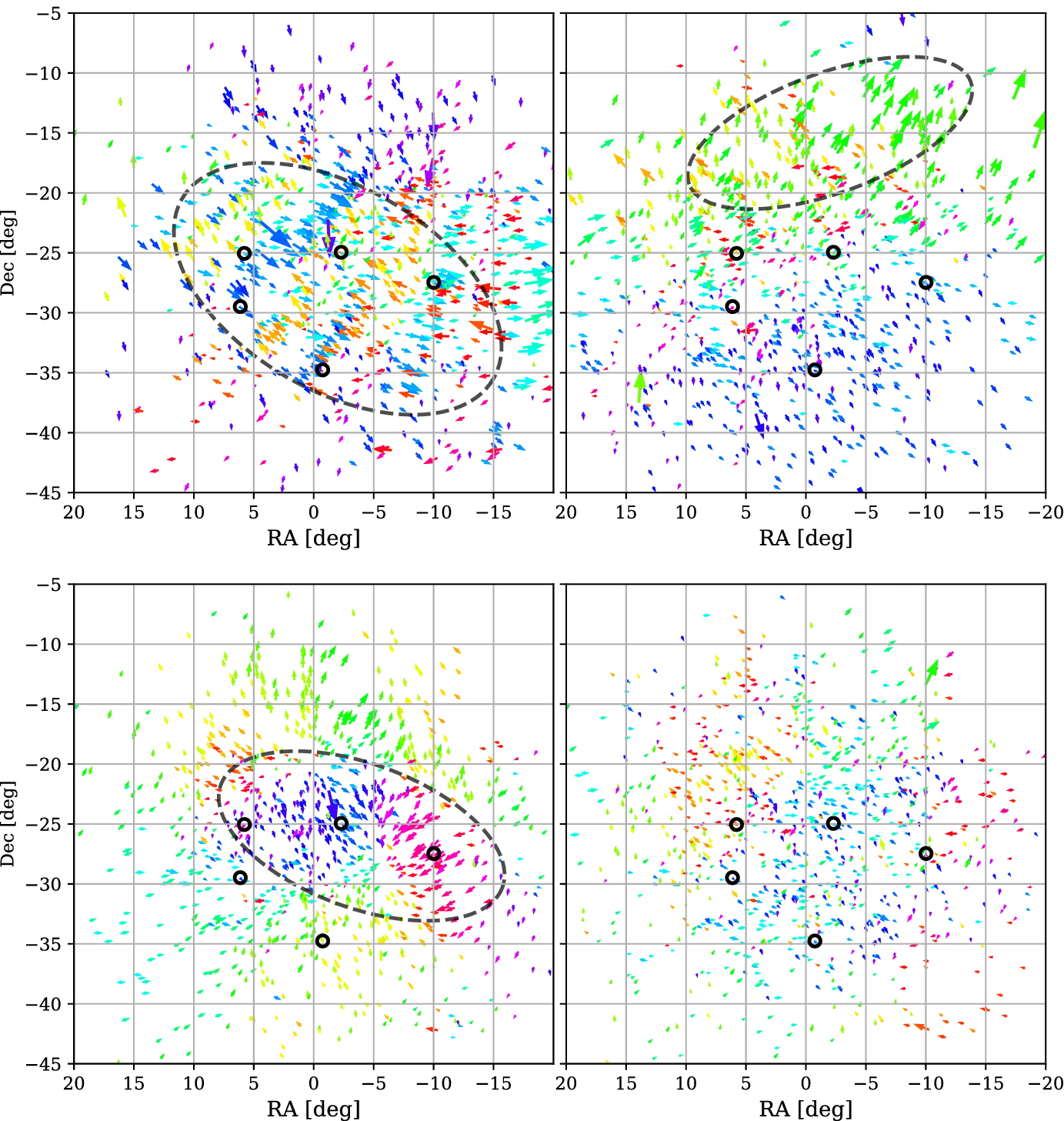
Figure 7. Plots of refractive shifts as measured by Jordan et al. (Reference Jordan2017) with each arrow representing the refractive shift of a source (arrows are also coloured by direction to emphasise structure). Circles indicate sources used for scintillation analysis. Two observations are shown for each of two TID events that were recorded in the data set, where the one above is the event from 2014 September 26 and below is from 2014 November 24. For each night, two observations are displayed; an observation from the middle of the night on the left, showing the TID at its most central and maximum intensity, and an observation from the end of the night on the right, once the TID has moved along. The ellipse marks the approximate location of the observed TIDs. For both events, the TID is clearly visible in the centre of the field on the leftmost plot. For the event of 2014 September 26, the TID continues to persist in the field, although it has moved upwards, and is no longer being sampled by the scintillating sources. For the event of 2014 November 24, the TID completely moves from the field by the end of the observation session.
The most conspicuous outliers from the Kolmogorov turbulence model have scintillation indices well below the level predicted from the measurements at larger scales: in other words, there is more structure on the larger scales. This is unsurprising given the regularity with which large, coherent structures which do not resemble turbulence are observed with the MWA (e.g. Loi et al. Reference Loi2015a). Indeed, Loi et al. (Reference Loi2016b) actually observed a case where a large-scale TID formed structures on scales of 10–100 km which persisted for at least two days; a picture fundamentally at odds with a turbulent cascade. However, this does raise the question of why, if these regular, large-scale structures do not imply structure on smaller scales, there is not an obvious anti-correlation between scintillation index and the anisotropy metric of Jordan et al. (Reference Jordan2017), which aims to quantify the extent to which structure is found on a particular scale. In particular (see Figure 8), observations with refractive shifts in the range $0.3^{\prime}$
–
$0.3^{\prime}$
– $0.5^{\prime}$
, where the scintillation indices are almost bimodal, it is the observations which obey the Kolmogorov relation that have the highest anisotropy values. Observations with extremely high scintillation indices (
$0.5^{\prime}$
, where the scintillation indices are almost bimodal, it is the observations which obey the Kolmogorov relation that have the highest anisotropy values. Observations with extremely high scintillation indices ( $m>0.1$
) are very highly structured according to the anisotropy metric (although the distribution of anisotropy as a function of refractive shift for observations with
$m>0.1$
) are very highly structured according to the anisotropy metric (although the distribution of anisotropy as a function of refractive shift for observations with $m>0.1$
appears identical to that for observations with
$m>0.1$
appears identical to that for observations with $0.05<m\le0.1$
).
$0.05<m\le0.1$
).
This apparent inconsistency may simply be an artefact of what the anisotropy metric is actually measuring. The left panel of Figure 7 shows the spatial distribution of refractive shifts during an observation where the refractive shifts are large, whereas the scintillation index (and anisotropy metric) are relatively small. The structure in the refractive shifts is characterised less by a preferred direction (which is what the anisotropy metric measures) and more by a lack of small-scale structures (shifts of nearby sources are strongly correlated). We therefore speculate that a different measurement of structure which measures the scale over which neighbouring sources are strongly correlated may show a clearer anti-correlation with scintillation index for a given level of ionospheric activity.
For the most extreme ionospheres observed here ( $\mathrm{refractive\ shift} > 0.4^{\prime}$
), the Kolmogorov spectrum occasionally underestimates the scintillation index by a factor of two or more (for a scattering height of 300 km). It may be that in these most extreme cases, the refractive shift for each source is actually varying over the 2-min observation, leading to an underestimate.
$\mathrm{refractive\ shift} > 0.4^{\prime}$
), the Kolmogorov spectrum occasionally underestimates the scintillation index by a factor of two or more (for a scattering height of 300 km). It may be that in these most extreme cases, the refractive shift for each source is actually varying over the 2-min observation, leading to an underestimate.
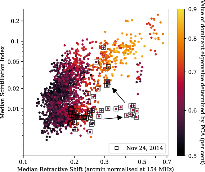
Figure 8. The median scintillation index calculated using the low-NSI sources in the brightest sources in the MWA EoR-0 field compared to the median refractive shift as recorded by Jordan et al. (Reference Jordan2017), with the level of anisotropy represented by the value of the dominant eigenvalue as determined by a principal component analysis (PCA). Arrows depict time progression of the observations throughout the night of the 2014 November 24; see Section 4.1 for further details.
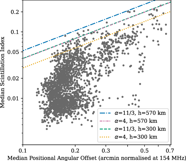
Figure 9. Relationship between refractive shift and scintillation index assuming power law turbulence. $11/3<\alpha\le4$
is the range of spectral indices found by Mevius et al. (Reference Mevius2016). Lower and upper limits on the height to the ionosphere, h, at 300 km (Hunsucker & Hargreaves Reference Hunsucker and Hargreaves2002; Wild & Roberts Reference Wild and Roberts1956) and 570 km (Loi et al. Reference Loi2015c), corresponding to Fresnel scales of 305 and 420 m respectively.
$11/3<\alpha\le4$
is the range of spectral indices found by Mevius et al. (Reference Mevius2016). Lower and upper limits on the height to the ionosphere, h, at 300 km (Hunsucker & Hargreaves Reference Hunsucker and Hargreaves2002; Wild & Roberts Reference Wild and Roberts1956) and 570 km (Loi et al. Reference Loi2015c), corresponding to Fresnel scales of 305 and 420 m respectively.
5.2 Implications for low-frequency radio astronomy
In measuring the very small scales of the ionosphere, we are probing the features which have the potential to have the most pernicious effects on radio astronomy. The presence of relatively large-scale structures revealed by refractive shifts places MWA calibrations in regime 2 as defined by Lonsdale (Reference Lonsdale2004) (see also Wijnholds et al. Reference Wijnholds, van der Tol, Nijboer and van der Veen2010), where the ionospheric irregularities are small compared to the field of view of the instrument, but large compared to the extent of the instrument. This means that corrections can be made in the image plane (Hurley-Walker & Hancock Reference Hurley-Walker and Hancock2018); although calibration and imaging algorithms also exist which allow direction-dependent corrections to be made while gridding the visibilities relatively efficiently, even when they vary quickly with time (van der Tol, Veenboer, & Offringa Reference van der Tol, Veenboer and Offringa2018).
On the other hand, significant structure on ${\sim}$
300 m scales (corresponding to an angular scale of a few arcminutes at typical ionosphere heights) would place calibration very firmly in a regime where the ionospheric phase would vary not just across the field of view, but across different parts of the array (Lonsdale Reference Lonsdale2004, regime 4). The ‘curse of dimensionality’ across pointing direction, array element location, and (with a modest drift velocity) time, means that the number of independent ionospheric complex gains (amplitude and phase) rapidly accumulates and may even outstrip the number of measurements; although the number of degrees of freedom may be reduced for a sufficiently dense observing array if assumptions can be made that the ionosphere is a thin and/or frozen screen, or has non-stochastic structure (Erickson Reference Erickson2005; Wijnholds et al. Reference Wijnholds, van der Tol, Nijboer and van der Veen2010).
${\sim}$
300 m scales (corresponding to an angular scale of a few arcminutes at typical ionosphere heights) would place calibration very firmly in a regime where the ionospheric phase would vary not just across the field of view, but across different parts of the array (Lonsdale Reference Lonsdale2004, regime 4). The ‘curse of dimensionality’ across pointing direction, array element location, and (with a modest drift velocity) time, means that the number of independent ionospheric complex gains (amplitude and phase) rapidly accumulates and may even outstrip the number of measurements; although the number of degrees of freedom may be reduced for a sufficiently dense observing array if assumptions can be made that the ionosphere is a thin and/or frozen screen, or has non-stochastic structure (Erickson Reference Erickson2005; Wijnholds et al. Reference Wijnholds, van der Tol, Nijboer and van der Veen2010).
Fortunately, the most extreme scintillation index in our work, 25%, implies a phase variance on the Fresnel scale of less than 0.1 rad $^2$
(Equation (6)) which is significant, but would have limited effects in the image plane except for strong sources. Nonetheless, more extended climatology of the small-scale structure in the ionosphere above the Murchison Radio Observatory, as well as more detailed observations to characterise its properties, may be useful in assessing the impact of these irregularities on future instruments such as the SKA-low and guiding future mitigation strategies.
$^2$
(Equation (6)) which is significant, but would have limited effects in the image plane except for strong sources. Nonetheless, more extended climatology of the small-scale structure in the ionosphere above the Murchison Radio Observatory, as well as more detailed observations to characterise its properties, may be useful in assessing the impact of these irregularities on future instruments such as the SKA-low and guiding future mitigation strategies.
5.3 Future work
We have limited our analysis to a straightforward comparison of median ionospheric scintillation index to existing per-observations metrics of ionospheric activity derived from the same data. Now that variability images have been generated for all these observations, more in-depth investigations would be possible using these data, such as breaking the field of view into subfields for a finer comparison of the refractive shifts and scintillation indices. The refractive shift data, in particular, is an extremely rich dataset which we have averaged down to two numbers per observation. If the distance to the irregularities is known (which can be determined by parallax: Loi et al. Reference Loi2015c) then these 2D fields of ionospheric gradients allow the structure function of the ionosphere to be determined from the separation of the closest detected sources (a few km) up to the field of view ( ${\sim}100$
km). Ionospheric scintillation provides a measurement on the smallest scale, with the approach of Rioja & Dodson (Reference Rioja and Dodson2022) potentially providing information on intermediate scales.
${\sim}100$
km). Ionospheric scintillation provides a measurement on the smallest scale, with the approach of Rioja & Dodson (Reference Rioja and Dodson2022) potentially providing information on intermediate scales.
We note that we have not used the full MWA for our scintillation analysis, but only a compact subarray of 36/128 elements. This demonstrates that ionospheric scintillation measurements could be made by instruments with much shorter baselines and less collecting area than the full MWA. For example, SKA-low prototype stations, co-located with the MWA could measure ionospheric scintillation with the significant advantage of all-sky coverage (Sokolowski et al. Reference Sokolowski2021).
The compact configuration of the MWA Phase II, which retains the core MWA antennas used for our scintillation measurements, but lacks the longer baselines that have been used in previous refractive shift measurements would also be capable of making scintillation measurements. This motivates us to consider whether ionospheric scintillation measurements can replace refractive shifts as the metric of activity where the latter is unavailable, or difficult to measure. If we choose a scintillation index of 2% to set our active vs. quiet threshold, we find that 1043/1447 (72%) Type I (‘quiet’) observations are below threshold, while 67, 48, 94% of observations are above threshold for Types II, III and IV respectively. Thus, ionospheric scintillation is a reasonable proxy for refractive shifts for assessing ionospheric activity, with only 21% of ‘active’ observations in total having a ‘false’ negative classification for ionospheric activity based on their scintillation. Whether the Type I observations with scintillation indices ${>}2$
% should be considered false positives for ionospheric activity or not depends on whether the structure on the Fresnel scale is a problem in itself. Chege et al. (Reference Chege2022) found tentative evidence that observations featuring Type I or III ionospheric activity have similar EoR power spectra; this suggests that the anisotropy metric is less important for the purposes of identifying poor, ionospherically contaminated observations. We note that the majority of the Type II false negatives have very large refractive shifts, so these might be identified even in data where refractive shifts cannot be measured as easily (such as MWA Phase II compact data; see Trott et al. Reference Trott2020). In this case, a combination of all 3 metrics may provide the best indication of ionospheric activity.
${>}2$
% should be considered false positives for ionospheric activity or not depends on whether the structure on the Fresnel scale is a problem in itself. Chege et al. (Reference Chege2022) found tentative evidence that observations featuring Type I or III ionospheric activity have similar EoR power spectra; this suggests that the anisotropy metric is less important for the purposes of identifying poor, ionospherically contaminated observations. We note that the majority of the Type II false negatives have very large refractive shifts, so these might be identified even in data where refractive shifts cannot be measured as easily (such as MWA Phase II compact data; see Trott et al. Reference Trott2020). In this case, a combination of all 3 metrics may provide the best indication of ionospheric activity.
Scintillation in the strong regime is more information-rich than weak scintillation due to its spectral structure. Fallows et al. (Reference Fallows2020) exploited this by applying pulsar scintillometry techniques (e.g. Stinebring et al. Reference Stinebring2001) to ionospheric scintillation data to reveal the height and velocity of two distinct scattering regions.
While the MWA cannot access the lower frequencies where strong ionospheric scintillation is common, the exceptionally large number of independent elements on spacings from ${\sim}10$
m–
${\sim}10$
m– ${\sim}6$
km may provide an alternative approach to deriving more detailed information from weak scattering. The layout of the MWA Phase II compact configuration, with 3 separate clusters of array elements, each
${\sim}6$
km may provide an alternative approach to deriving more detailed information from weak scattering. The layout of the MWA Phase II compact configuration, with 3 separate clusters of array elements, each ${\sim}$
100 m in diameter raises the possibility of using each cluster to perform a ‘multi-station’ analysis. This is a standard technique in IPS, pioneered by Dennison & Hewish (Reference Dennison and Hewish1967), which was also used to confirm that scintillation due to the interstellar medium was responsible for the intraday variability phenomenon (Jauncey et al. Reference Jauncey2000). It involves measuring the scintillation signature at different geographical locations. These signals are then cross-correlated, and any delay between them can be attributed to the time it takes for the scintillation pattern to drift from one location to another. With the MWA in compact configuration, the three clusters would be treated as independent sub-arrays. Any co-located instruments capable of measuring ionospheric scintillation, such as SKA-low prototype stations, could also be used without any requirement that they be interferometrically correlated with the MWA. As well as the tiles that make up the MWA Phase II compact configuration, a Radio Array of Portable Interferometric Detectors (RAPID Lind et al. Reference Lind, Lonsdale, Faulkner, Alexander and Mattmann2013) or the SKA-low in a mode where each station is treated as a separate interferometer could be used in this way to measure scintillation pattern on the ground. Since this would be an independent and direct measurement of the Fresnel scale, it could be combined with the amplitude scintillation index to determine the height of the irregularities.
${\sim}$
100 m in diameter raises the possibility of using each cluster to perform a ‘multi-station’ analysis. This is a standard technique in IPS, pioneered by Dennison & Hewish (Reference Dennison and Hewish1967), which was also used to confirm that scintillation due to the interstellar medium was responsible for the intraday variability phenomenon (Jauncey et al. Reference Jauncey2000). It involves measuring the scintillation signature at different geographical locations. These signals are then cross-correlated, and any delay between them can be attributed to the time it takes for the scintillation pattern to drift from one location to another. With the MWA in compact configuration, the three clusters would be treated as independent sub-arrays. Any co-located instruments capable of measuring ionospheric scintillation, such as SKA-low prototype stations, could also be used without any requirement that they be interferometrically correlated with the MWA. As well as the tiles that make up the MWA Phase II compact configuration, a Radio Array of Portable Interferometric Detectors (RAPID Lind et al. Reference Lind, Lonsdale, Faulkner, Alexander and Mattmann2013) or the SKA-low in a mode where each station is treated as a separate interferometer could be used in this way to measure scintillation pattern on the ground. Since this would be an independent and direct measurement of the Fresnel scale, it could be combined with the amplitude scintillation index to determine the height of the irregularities.
An alternative approach, which would be applicable to both configurations of the MWA, as well as the future SKA-low, would be to measure scintillation via its effect on the complex visibilities. The theory, as developed by Cronyn (Reference Cronyn1972), shows that for an interferometer which fully samples the scintillation pattern on the ground (i.e. baselines cover a range of values around the Fresnel scale at a range of orientations) the complex visibilities encode not only the strength of scattering but the velocity vector, and even the form of the structure function from the Fresnel scale up to the length of the longest baseline. Such an approach would, however, likely require observation of a source that is sufficiently bright as to dominate the visibilities.
5.4 Conclusions
We have used ionospheric scintillation in the weak regime to measure the structure of the ionosphere on scales $r_{\text{F}}\sim$
300 m. In the most extreme case observed, the phase variance on this scale was 0.06 rad
$^2$
at our observing frequency of 154 MHz.
$r_{\text{F}}\sim$
300 m. In the most extreme case observed, the phase variance on this scale was 0.06 rad
$^2$
at our observing frequency of 154 MHz.The scintillation index is highly correlated (Pearson correlation coefficient 0.71) with refractive shifts measured on a baseline
${\sim}2$
km. The relationship between these two metrics suggests that Kolmogorov turbulence is the dominant structure in the ionosphere on scales 300–2000 m, at least in more active ionospheric conditions.There are a number of observations for which non-turbulent, large-scale structures appear to dominate, but these do not necessarily show anisotropy (and high scintillation indices are also seen when the large-scale structure is highly isotropic)
In the most extreme ionospheric conditions, refractive shifts underestimate the small-scale variance by a factor of four or more.
The more extreme conditions seen in our data could have significant, if manageable, effects on radio astronomy observations. There is much scope and incentive for future work, both to increase our understanding of the mid-latitude ionosphere, and the effects that it may have on trans-ionospheric observations.


Acknowledgements
We would like to thank C. Trott for useful discussions regarding the comparison between scintillation and refractive shift measurements. A. W acknowledges the invaluable support of an ICRAR summer studentship. This scientific work makes use of the Murchison Radio-astronomy Observatory, operated by CSIRO. We acknowledge the Wajarri Yamatji people as the traditional owners of the Observatory site. Support for the operation of the MWA is provided by the Australian Government (NCRIS), under a contract to Curtin University administered by Astronomy Australia Limited. We acknowledge the Pawsey Supercomputing Centre which is supported by the Western Australian and Australian Governments.


 Open access