


1. Introduction
Wave turbulence theory (WTT) is a framework for describing the long-time statistical behaviour of fields of many weakly interacting waves. In such a system, over scales far from those of forcing and dissipation, self-similar wave–wave interactions drive an energy cascade between scales and lead to the development of a power-law spectrum. While wave turbulence shares much phenomenology with hydrodynamic turbulence, WTT enables an analytic treatment of the governing wave equation through which the evolution equation of the wave spectrum can be derived, yielding as a stationary solution the full functional form of the power-law spectrum. Due to the ubiquity of nonlinear waves in nature, WTT has found use in a diverse array of fields, including magnetohydrodynamics (Galtier et al. Reference Galtier, Nazarenko, Newell and Pouquet2000; Galtier Reference Galtier2014), physical oceanography (Zakharov & Filonenko Reference Zakharov and Filonenko1967; Zakharov Reference Zakharov1968), acoustics (L'vov et al. Reference L'vov, L'vov, Newell and Zakharov1997), astrophysics (Galtier & Nazarenko Reference Galtier and Nazarenko2017, Reference Galtier and Nazarenko2021), and others.
One of the primary results of WTT is the derivation of the wave kinetic equation (WKE) directly from the governing dynamical equations. Formulated under assumptions on high-order field statistics in the kinetic limit (of a large domain and small nonlinearity), the WKE expresses the time evolution of wave action spectral density as an integral over wave–wave interactions. The WKE also has an inertial-range stationary solution of wave action  $n(k)\sim P^{\theta }k^{\gamma }$, where $k$ is the wavenumber, $P$ is the energy flux of the forward cascade, and $\theta$ and $\gamma$ are scaling exponents. Over the decades, many efforts have been made to study numerically and experimentally the scaling exponent $\gamma$ for a wide variety of physical systems (e.g. Nazarenko & Onorato Reference Nazarenko and Onorato2006; Denissenko, Lukaschuk & Nazarenko Reference Denissenko, Lukaschuk and Nazarenko2007; Miquel, Alexakis & Mordant Reference Miquel, Alexakis and Mordant2014; Düring, Josserand & Rica Reference Düring, Josserand and Rica2017; Hassaini & Mordant Reference Hassaini and Mordant2018; Monsalve et al. Reference Monsalve, Brunet, Gallet and Cortet2020). The exponent $\theta$, and in general the properties of $P$, are, however, much less studied, despite the fact that they are more relevant to the formulation of the WKE. A small number of existing works on the scaling of $P$ (e.g. Falcon, Laroche & Fauve Reference Falcon, Laroche and Fauve2007; Deike, Berhanu & Falcon Reference Deike, Berhanu and Falcon2014a; Pan & Yue Reference Pan and Yue2014) sometimes produce inconsistent conclusions, partly because of their indirect measurements of $P$ based on the energy input/dissipation rate. Given a non-stationary spectrum (say in the free-decay case) or broad-scale dissipation of the wave field (which results in significant dissipation in the inertial range), it is not guaranteed that these measurements of $P$ based on the input/dissipation rate reflect the true dynamics of inter-scale energy cascade (see detailed analysis in Deike et al. Reference Deike, Berhanu and Falcon2014a; Pan & Yue Reference Pan and Yue2015).
A more direct approach for the exact evaluation of  $P$ can be formulated through the nonlinear terms in the governing equation that are responsible for the wave–wave interactions leading to the energy cascade (e.g. Hrabski & Pan Reference Hrabski and Pan2020). This approach allows the resolution of the probability distribution of $P$ at arbitrary scales that is not obtainable by previous input/dissipation-based methods. Moreover, this formulation enables a decomposition of the energy flux into contributions from exact- and quasi-resonances. In particular, we can perform a quartet-level decomposition of $P=\sum _{\varOmega } P_{\varOmega }$, with $P_{\varOmega }$ representing contributions from a set of quartets with frequency mismatch $\varOmega$. This decomposition technique will allow us to elucidate many mechanisms underlying the scaling and distribution of $P$, and provide a direct measure of nonlinear broadening by evaluating the contribution of quasi-resonances to the energy cascade. This new measure of nonlinear broadening can be more direct and physically intuitive than previous approaches based on the coherence function (e.g. Aubourg & Mordant Reference Aubourg and Mordant2015; Pan & Yue Reference Pan and Yue2017; Zhang & Pan Reference Zhang and Pan2021) or the broadened dispersion relation (e.g. Mordant Reference Mordant2010; Deike et al. Reference Deike, Fuster, Berhanu and Falcon2014b).
Another study enabled by this decomposition technique is one on the WTT closure model, which relates the high-order correlators (of frequency mismatch  $\varOmega$) to the product of pair correlators. This relation is usually argued in conjunction with a broadening function $f(\varOmega )$ that approaches the delta function $\delta (\varOmega )$ at the kinetic limit (Nazarenko Reference Nazarenko2011; Zakharov, L'vov & Falkovich Reference Zakharov, L'vov and Falkovich2012; Buckmaster et al. Reference Buckmaster, Germain, Hani and Shatah2021; Deng & Hani Reference Deng and Hani2021a,Reference Deng and Hanib). We are particularly interested in the form of $f(\varOmega )$ in a finite domain, which is more relevant to the situations in many numerical simulations and experiments. Interesting attempts in this direction include the development of a generalized kinetic equation (by implementing a numerical solution to the closure) (Annenkov & Shrira Reference Annenkov and Shrira2006), which, however, does not focus on the functional form $f(\varOmega )$ in the stationary state of wave turbulence. A lack of understanding of the closure problem is a major obstacle to advancement in the theory of wave turbulence; for example, the obvious contradiction between the Majda–McLaughlin–Tabak (MMT) closure and WTT closure (as well as the elusive numerical observations) raised more than 20 years ago is still not understood fully today (Majda, McLaughlin & Tabak Reference Majda, McLaughlin and Tabak1997; Cai et al. Reference Cai, Majda, McLaughlin and Tabak1999; Zakharov et al. Reference Zakharov, Guyenne, Pushkarev and Dias2001).
The purpose of this paper, in general, is to establish a methodology such that all aforementioned analysis (including various properties of energy flux and the closely-related closure problem) can be studied directly using numerical data from simulations of the governing equations. We demonstrate our methodology in the context of a two-dimensional (2-D) variant of the MMT equation with the Schrödinger-like dispersion relation  $\omega (k)=k^2$. This system is chosen in part to continue the work of the authors Hrabski & Pan (Reference Hrabski and Pan2020), but also to aid in the development of a methodology useful to many fluid systems. The use of such a toy model removes some of the complexities associated with real fluid systems (e.g. the non-resonant quadratic nonlinearity of surface gravity waves), while retaining the essential nonlinear interactions of wave turbulence that are common to all wave systems in fluids.
We now summarize the main results of the paper. In a stationary state of MMT turbulence, our analysis shows that the energy flux  $P$, as a time series, closely follows a Gaussian distribution, with a standard deviation several times its mean value $\bar {P}$. The large standard deviation of $P$ is found to be dominated by fluctuations in time of the quasi-resonant components $P_{\varOmega \neq 0}$. The scaling between the spectral level and $\bar {P}$ shows a $\bar {P}^{1/3}$ dependence at high nonlinearity levels, and transits to $\bar {P}^{1/2}$ dependence at low nonlinearity levels. The $\bar {P}^{1/3}$ scaling is consistent with the kinetic scaling and is established when $\bar {P}$ is dominated by the quasi-resonant contributions. This is, in fact, consistent with the physical picture that the WKE represents a state dominated by quasi-resonances at the kinetic limit. The $\bar {P}^{1/2}$ scaling is consistent with the dynamic scaling derived from the MMT equation, established as a result of the dominance of exact resonances in $\bar {P}$. Finally, the WTT closure model on the fourth-order correlator, when evaluated in a time window of $O(500)$ fundamental periods, is found to be not valid on the individual quartet level. When we increase the number of quartets to the level at which $P$ is formulated ( $O(10^9)$ number of quartets for each $\varOmega$), the average behaviour of the fourth-order correlator lies much closer to WTT closure, but with $f(\varOmega )\sim 1/\varOmega ^\beta$ (with $\beta$ between 1.3 and 1.6) observed instead of the previously argued functions from WTT.
2. Formulation of energy flux for the MMT model
We consider a 2-D MMT model (Majda et al. Reference Majda, McLaughlin and Tabak1997) that has been used widely to study wave turbulence problems (Cai et al. Reference Cai, Majda, McLaughlin and Tabak1999; Zakharov et al. Reference Zakharov, Guyenne, Pushkarev and Dias2001; Chibbaro, De Lillo & Onorato Reference Chibbaro, De Lillo and Onorato2017; Sheffield & Rumpf Reference Sheffield and Rumpf2017). The model describes the evolution of a complex scalar  $\psi (\boldsymbol {x},t)$:
 \begin{equation} \mathrm{i}\,\frac{\partial \psi}{\partial t} = |\partial_{\boldsymbol{x}}|^\alpha\psi + |\partial_{\boldsymbol{x}}|(| |\partial_{\boldsymbol{x}}|\psi|^2|\partial_{\boldsymbol{x}}|\psi),\end{equation}
where  $\boldsymbol {x}$ gives the 2-D spatial coordinates and $t$ is time, and the operator $|\partial _{\boldsymbol {x}}|^{\alpha }\psi$ corresponds to the multiplication of each Fourier component $\hat {\psi }_{\boldsymbol {k}}$ by $k^{\alpha }$, with $k$ being the magnitude of wavenumber vector $\boldsymbol {k}$. We choose $\alpha =2$, yielding a dispersion relation $\omega _{k}=k^2$ that is the same as the nonlinear Schrödinger equation (NLSE). In fact, our model differs from the 2-D NLSE by the addition of derivatives to the nonlinear term, which provide accelerated evolution to the stationary state (Falkovich & Shafarenko Reference Falkovich and Shafarenko1991). The system conserves the Hamiltonian $H = H_{l} + H_{nl}$, with the linear and nonlinear parts defined as
 \begin{equation} \left.\begin{array}{c@{}}
\displaystyle H_{l} =
\int\bigl||\partial_{\boldsymbol{x}}|\psi\bigr|^{2} \, {\rm d}\kern0.06em \boldsymbol{x}, \\ \displaystyle H_{nl} =
\dfrac{1}{2}\int
\bigl||\partial_{\boldsymbol{x}}|\psi\bigr|^{4} \, {\rm d}\kern0.06em \boldsymbol{x}, \end{array}\right\}
\end{equation}
\begin{equation} \left.\begin{array}{c@{}}
\displaystyle H_{l} =
\int\bigl||\partial_{\boldsymbol{x}}|\psi\bigr|^{2} \, {\rm d}\kern0.06em \boldsymbol{x}, \\ \displaystyle H_{nl} =
\dfrac{1}{2}\int
\bigl||\partial_{\boldsymbol{x}}|\psi\bigr|^{4} \, {\rm d}\kern0.06em \boldsymbol{x}, \end{array}\right\}
\end{equation}
and the total action  $\|\psi \|_2 = \int |\psi |^{2} \, \textrm {d} \boldsymbol {x}$.
2.1. Exact formulations of instantaneous energy flux  $P(t)$

In this section, we provide the exact formulation of  $P(t)$, defined as the flux of spectral energy (i.e. $\omega _{k}\hat {\psi }_{\boldsymbol {k}}\hat {\psi }_{\boldsymbol {k}}^*$ without the high-order component) across arbitrary wavenumber $k_b$. We consider (2.1) on a torus of size $2{\rm \pi} \times 2{\rm \pi}$, such that $\boldsymbol {k}$ is composed of only integers. We then make an energy conservation argument over a control volume $k< k_b$ in spectral space:
 \begin{equation} P(t) ={-}\sum_{ \boldsymbol{k}\in \{ \boldsymbol{k}|k< k_b \} }\omega_{k}\,\frac{\partial(\hat{\psi}_{\boldsymbol{k}}\hat{\psi}_{\boldsymbol{k}}^*)}{\partial t}(t) ={-} \sum_{ \boldsymbol{k}\in \{ \boldsymbol{k}|k< k_b \} }\omega_{k}\left( \frac{\partial\hat{\psi}_{\boldsymbol{k}}}{\partial t}\,\hat{\psi}_{\boldsymbol{k}}^* + \frac{\partial \hat{\psi}_{\boldsymbol{k}}^*}{\partial t}\, \hat{\psi}_{\boldsymbol{k}}\right)(t). \end{equation}
By substituting the Fourier domain representation of (2.1) into (2.3), we see that the linear term in (2.1) does not contribute to  $P(t)$, and a simple manipulation of the nonlinear term yields
 \begin{equation} P(t) ={-}\sum_{ \boldsymbol{k}\in \{ \boldsymbol{k}|k< k_b \} }\omega_{k} \sum_{(\boldsymbol{k}_{1}, \boldsymbol{k}_{2}, \boldsymbol{k}_{3})\in S_{\boldsymbol{k}}} 2 k_1 k_2 k_3 k\,{\rm Im}(\hat{\psi}_{\boldsymbol{1}} \hat{\psi}_{\boldsymbol{2}} \hat{\psi}_{\boldsymbol{3}}^* \hat{\psi}_{\boldsymbol{k}}^*)(t), \end{equation}
where  $S_{\boldsymbol {k}}$ is the set of all $(\boldsymbol {k}_{1}, \boldsymbol {k}_{2}, \boldsymbol {k}_{3})$ with $\boldsymbol {k}_{1} + \boldsymbol {k}_{2} - \boldsymbol {k}_{3} - \boldsymbol {k}=0$. We note that (2.4) is exact even if forcing and dissipation are added to (2.1) (which may affect (2.3) but not (2.4)), because only the nonlinear term in (2.1) is responsible for the inter-scale energy flux. Taking the wave action $n({\boldsymbol {k}})\sim |\hat {\psi }_{\boldsymbol {k}}|^2$, (2.4) implies a dynamic scaling of $n\sim P^{1/2}$ via a heuristic argument. This is a result of using directly the dynamic equation (2.1) to formulate the energy flux.
With (2.4) available, we can further perform a decomposition  $P(t)=\sum _{\varOmega } P_{\varOmega }(t)$ by partitioning the set $S_{\boldsymbol {k}}$ according to the frequency mismatch of each quartet interaction. Specifically, defining $S_{\varOmega, \boldsymbol {k}} \equiv \ \{ (\boldsymbol {k}_1, \boldsymbol {k}_2, \boldsymbol {k}_3) \in S_{\boldsymbol {k}} \mid |\omega _{1}+\omega _{2}-\omega _{3}-\omega _{k}| = \varOmega \}$, we have $\bigcup _{\varOmega } S_{\varOmega,\boldsymbol {k}} = S_{\boldsymbol {k}}$ with all sets $S_{\varOmega,\boldsymbol {k}}$ disjoint. Therefore, $P_{\varOmega }(t)$ can be formulated naturally as
 \begin{equation} P_\varOmega(t) ={-}\sum_{ \boldsymbol{k}\in \{ \boldsymbol{k}|k< k_b \} } \omega_{k} \sum_{(\boldsymbol{k}_{1}, \boldsymbol{k}_{2}, \boldsymbol{k}_{3})\in S_{\varOmega , \boldsymbol{k}}} 2 k_1 k_2 k_3 k\, {\rm Im}(\hat{\psi}_{\boldsymbol{1}} \hat{\psi}_{\boldsymbol{2}} \hat{\psi}_{\boldsymbol{3}}^* \hat{\psi}_{\boldsymbol{k}}^*)(t).\end{equation}
The computation using (2.5) allows us to measure the contribution to  $P$ from resonances with different $\varOmega$, as well as to separate the quasi-resonant and exact-resonant contributions by $P_{\varOmega >0}$ and $P_{\varOmega =0}$, respectively.
2.2. Formulations of energy flux under the WTT closure
The WTT closure for (2.1) relates the fourth-order correlator to pair correlators by
 \begin{equation} {\rm Im} \overline{(\hat{\psi}_{\boldsymbol{1}} \hat{\psi}_{\boldsymbol{2}}\hat{\psi}_{\boldsymbol{3}}^{*} \hat{\psi}_{\boldsymbol{k}}^{*})}_{\varOmega} = 2 k k_1 k_2 k_3 (n_{\boldsymbol{1}} n_{\boldsymbol{2}} n_{\boldsymbol{3}} + n_{\boldsymbol{1}} n_{\boldsymbol{2}} n_{\boldsymbol{k}} - n_{\boldsymbol{1}} n_{\boldsymbol{k}} n_{\boldsymbol{3}} - n_{\boldsymbol{k}} n_{\boldsymbol{2}} n_{\boldsymbol{3}})\,f(\varOmega), \end{equation}
where an overbar denotes the ensemble average (or time average in numerical analysis), and  $n_{\boldsymbol {k}} = \overline {\hat {\psi }_{\boldsymbol {k}} \hat {\psi }^*_{\boldsymbol {k}}}$ is wave action. We also use a subscript $\varOmega$ for $\textrm {Im} \overline {(\hat {\psi }_{\boldsymbol {1}}\hat {\psi }_{\boldsymbol {2}} \hat {\psi }_{\boldsymbol {3}}^{*}\hat {\psi }_{\boldsymbol {k}}^{*})}_{\varOmega }$ to denote the frequency mismatch of the corresponding four wave modes. The closure (2.6) has been derived in various (heuristic) ways in the traditional WTT literature (Hasselmann Reference Hasselmann1962; Janssen Reference Janssen2003; Zakharov et al. Reference Zakharov, L'vov and Falkovich2012; Pan Reference Pan2017) by assuming quasi-Gaussian statistics and that the nonlinear time scale is much longer than the linear time scale. In more recent works, however, it has been shown that the quasi-Gaussian assumption can be dropped, and the WKE can be derived instead assuming random phases and amplitudes (Choi, Lvov & Nazarenko Reference Choi, Lvov and Nazarenko2005a; Choi et al. Reference Choi, Lvov, Nazarenko and Pokorni2005b; Eyink & Shi Reference Eyink and Shi2012; Chibbaro, Dematteis & Rondoni Reference Chibbaro, Dematteis and Rondoni2018). Depending on different methods of the derivation, $f(\varOmega )$ takes the form of $\epsilon /(\varOmega ^2+\epsilon ^2)$ (Zakharov et al. Reference Zakharov, L'vov and Falkovich2012) or a sinc-like function (particularly $\sin (\varOmega t)/\varOmega$ as in Janssen (Reference Janssen2003) and $\sin ^2(\varOmega t)/\varOmega ^2$ as in Nazarenko (Reference Nazarenko2011)). We note here that in all these derivations, the function $f$ depends only on $\varOmega$, and not on the wavenumbers of the quartet. The WKE is then derived in the limit of the parameters $\epsilon \rightarrow 0$ and $t\rightarrow \infty$ for the first and second cases, respectively, with both leading to $f(\varOmega )\rightarrow {\rm \pi}\,\delta (\varOmega )$.
We are interested in the performance of the closure (2.6) in computing the energy flux  $P_\varOmega$. For this purpose, we substitute (2.6) into the average of (2.5) to obtain
 \begin{align} \bar{P}_{\varOmega} &={-}\sum_{ \boldsymbol{k}\in \{ \boldsymbol{k}|k< k_b \} } \omega_{k} \nonumber\\ &\quad \times \sum_{(\boldsymbol{k}_{1}, \boldsymbol{k}_{2}, \boldsymbol{k}_{3})\in S_{\varOmega , \boldsymbol{k}}} 4 k_1^2 k_2^2 k_3^2 k^2 (n_{\boldsymbol{1}} n_{\boldsymbol{2}} n_{\boldsymbol{3}} + n_{\boldsymbol{1}} n_{\boldsymbol{2}} n_{\boldsymbol{k}} - n_{\boldsymbol{1}} n_{\boldsymbol{k}} n_{\boldsymbol{3}} - n_{\boldsymbol{k}} n_{\boldsymbol{2}} n_{\boldsymbol{3}} )\,f(\varOmega). \end{align}
The question in (2.6) and (2.7) is whether there exists a form of  $f(\varOmega )$ consistent with WTT such that the equality holds in the two equations. To investigate this, we will evaluate in § 4 the functional form $f(\varOmega )$ in both (2.6) and (2.7) using our numerical data to compute all the other terms in the two equations (e.g. $\bar {P}_{\varOmega }$ in (2.7) can be computed through the time average of (2.5)). The difference between the two evaluations of $f(\varOmega )$ is that the latter involves the sum of an enormous number of interactions while the former is for an individual quartet. Through comparison of the numerically resolved $f(\varOmega )$ with their WTT counterparts, the validity of the WTT closure can be assessed.
3. Set-up of numerical experiments
We compute the solution to (2.1) via a pseudospectral method on a periodic domain of size  $2{\rm \pi} \times 2{\rm \pi}$ containing $512\times 512$ modes. In our previous work (Hrabski & Pan Reference Hrabski and Pan2020), we have shown that an increase to $1024\times 1024$ modes does not change the inertial range spectrum. The linear term of (2.1) is integrated analytically to reduce the system stiffness, while the nonlinear term is integrated via an explicit fourth-order Runge–Kutta scheme. Our purpose is to generate a long stationary state so that the distributions of $P$ (and other quantities discussed in § 2) are sufficiently resolved. Therefore, we force the system at large scales (in conjunction with small-scale dissipation) instead of considering free-decay turbulence. Specifically, we add a forcing term
 \begin{equation} F = \left\{
\begin{array}{@{}ll}
F_{r}+\mathrm{i}F_{i}, & 7\le
k\le9, \\ 0, & {\rm otherwise},
\end{array} \right.\end{equation}
\begin{equation} F = \left\{
\begin{array}{@{}ll}
F_{r}+\mathrm{i}F_{i}, & 7\le
k\le9, \\ 0, & {\rm otherwise},
\end{array} \right.\end{equation}
to the right-hand side of (2.1), with  $F_{r}$ and $F_{i}$ taken from a zero-mean Gaussian distribution, which results in a standard white-noise forcing in time with amplitude variance proportional to the size of the time step. Dissipation is accounted for by adding two terms
 \begin{equation} \left. \begin{array}{c@{}}
D_1 = \left\{ \begin{array}{@{}ll@{}}
-\mathrm{i}\nu_1
\hat{\psi}_{\boldsymbol{k}}, & k\ge100,
\\ 0, & {\rm otherwise},
\end{array} \right. \\ D_2 = \left\{
\begin{array}{@{}ll@{}} -\mathrm{i}\nu_2
\hat{\psi}_{\boldsymbol{k}}, & k\le7, \\
0, & {\rm otherwise}, \end{array}
\right.
\end{array}\right\}\end{equation}
\begin{equation} \left. \begin{array}{c@{}}
D_1 = \left\{ \begin{array}{@{}ll@{}}
-\mathrm{i}\nu_1
\hat{\psi}_{\boldsymbol{k}}, & k\ge100,
\\ 0, & {\rm otherwise},
\end{array} \right. \\ D_2 = \left\{
\begin{array}{@{}ll@{}} -\mathrm{i}\nu_2
\hat{\psi}_{\boldsymbol{k}}, & k\le7, \\
0, & {\rm otherwise}, \end{array}
\right.
\end{array}\right\}\end{equation}
at small and large scales, respectively, with the latter included to prevent energy accumulation at large scales due to the inverse cascade. The parameters in (3.2) are chosen to be  $\nu _1 = 6\times 10^{-12} (k-100)^{8}$ and $\nu _2 = 30 k^{-4}$ throughout all the simulations. Forcing and dissipation of this type have been demonstrated to produce results compatible with the WTT predictions in the one-dimensional MMT model (Cai et al. Reference Cai, Majda, McLaughlin and Tabak1999).
In addition, to accelerate convergence to the stationary state, we start the simulations from initial conditions  $\hat {\psi }_{\boldsymbol {k}}=a_0\, \textrm {e}^{-0.1|k-10|+\mathrm {i}\phi _{\boldsymbol {k}}}$, with $\phi _{\boldsymbol {k}}$ the uniformly-distributed, decorrelated random phases, and $a_0$ a real constant chosen to provide an energy close to that of the expected stationary state. To obtain the scaling $\theta$ over a range of $\bar {P}$, we run a collection of 19 simulations, differing only in forcing strength $\sigma ^2_F$ and initial spectral level $a_0$. These simulations cover a range of $\bar {P}$ spanning several orders of magnitude, with data collected in the stationary state for each case.
4. Results
Before presenting the results on energy flux, we first check the spectra at stationary states in simulations with different forcing magnitudes. Several typical one-dimensional angle-averaged spectra  $n(k)$ at different levels are shown in figure 1(a), where we observe power-law ranges close to one decade for all spectra. Figure 1(b) shows the power-law exponent $\gamma$ evaluated in all 19 simulations via a least-squares fit in $k\in [13,60]$, as a function of the spectral level computed by an integral measure of the (conservatively taken) power-law range
 \begin{equation} N = \sum_{ \boldsymbol{k}\in \{ \boldsymbol{k}|13< k<60 \} } n_{\boldsymbol{k}}. \end{equation}
We note that  $N$, as a measure of nonlinearity level, is monotonically related to the measure $\varepsilon \equiv H_{nl}/H_l$ (see details in the Appendix) in the range of $N$ in figure 1(b), corresponding to $\varepsilon \in [0.002,0.03]$ (a range where the linear part $H_l$ dominates the total Hamiltonian).

Figure 1. (a) A representative collection of fully-developed, angle-averaged wave action spectra  $n(k)$. (b) Spectral slope $\gamma$ as a function of $N$, with WTT value $\gamma _0=-4.67$ (dashed line).
We see in figure 1(b) that  $\gamma$ increases (i.e. the spectrum becomes shallower) with the decrease of $N$, reaching the WTT prediction $\gamma _0=-4.67$ for low spectral levels (in particular, $\gamma _0=-2s/3-d$ with $d=2$ the dimension and $s=4$ the degree of homogeneity of the interaction kernel, as in Nazarenko Reference Nazarenko2011). This behaviour of $\gamma$ is consistent with our previous study of the free-decay MMT turbulence (except that use of different dissipation schemes may have some slight effect). As analysed by the authors Hrabski & Pan (Reference Hrabski and Pan2020), the fact that $\gamma \rightarrow \gamma _0$ for small $N$ is (partly) a result of the dispersion relation $\omega _k=k^2$, which leads to a continuous resonant system (to be discussed in § 4.2) at low nonlinearity (Faou, Germain & Hani Reference Faou, Germain and Hani2016). The deviation of $\gamma$ from $\gamma _0$ at high nonlinearity may result from coherent structures, as suggested by Zakharov et al. (Reference Zakharov, Guyenne, Pushkarev and Dias2001) and Chibbaro et al. (Reference Chibbaro, De Lillo and Onorato2017) in the one-dimensional context, or some features of the 2-D MMT model that are yet to be fully understood. For waves in different physical contexts, e.g. surface gravity waves (Denissenko et al. Reference Denissenko, Lukaschuk and Nazarenko2007; Zhang & Pan Reference Zhang and Pan2021) and capillary waves (Pushkarev & Zakharov Reference Pushkarev and Zakharov2000; Pan & Yue Reference Pan and Yue2014), the behaviours of $\gamma$ are remarkably different.
We next present our full study of energy flux, with results organized into three subsections. Subsection 4.1 discusses the distributions of  $P$ and its associated decomposition $P_\varOmega$. Subsection 4.2 focuses on the scaling of spectral level with $P$, with the results explained by the contributions of quasi/exact-resonances to $P$. The study related to the closure model is then presented in § 4.3.
4.1. Flux distributions and decomposition
A typical distribution of energy flux  $P(t)$, computed with $k_b=30$ from $2^{16}$ data points over a time window of $T_w=256T_0$, is shown in figure 2(a) (with $T_0=2{\rm \pi}$ the fundamental period corresponding to the longest wave in the domain). We find that $P$ follows closely a Gaussian distribution, with standard deviation $\sigma (P)=621.8$, several times larger than the mean value $\bar {P}=77.02$. The very large standard deviation is consistent with previous studies in wave turbulence (Falcon et al. Reference Falcon, Aumaître, Falcón, Laroche and Fauve2008) and hydrodynamic turbulence (Bandi et al. Reference Bandi, Goldburg, Cressman and Pumir2006). However, the nearly perfect Gaussian form of the distribution has not been observed in these previous works, possibly because of differing turbulent systems and their different way of evaluating $P$. In addition, our method allows us to study the fully-resolved distribution of $P$ at any scale (i.e. with arbitrary $k_b$). In figures 2(b) and 2(c), we plot the values of $\bar {P}$ and $\sigma (P)$ for $k_b$ varying in the inertial range from 20 to 90. The mean flux $\bar {P}$ remains almost constant for all $k_b$, which is consistent with the WTT constant flux argument in the inertial range (this is possible only by avoiding broad-scale dissipation in simulations). The standard deviation $\sigma (P)$ increases with $k_b$, because more quartet interactions are included (as $k$ becomes denser), resulting in more fluctuations in $P(t)$. We also include in figures 2(a) and 2(b) the energy flux $\bar {P}$ computed from the high-wave-number dissipation rate,
 \begin{equation} \bar{P}_d = \sum_{ \boldsymbol{k}\in \{ \boldsymbol{k}|k>100 \} }\nu_1 \omega_{k} \overline{\hat{\psi}_{\boldsymbol{k}} \hat{\psi}_{\boldsymbol{k}}^*},\end{equation}
which agrees well with the majority of values of  $\bar {P}$, especially for larger $k_b$ (to a relative difference within $O(1\,\%)$). Because of this, we will use $\bar {P}_d$ to represent the values of $\bar {P}$ for all 19 simulations in the subsequent analysis, since $P_d$ yields a faster calculation due to an easier formulation and much smaller fluctuations (requiring fewer data points for averaging).
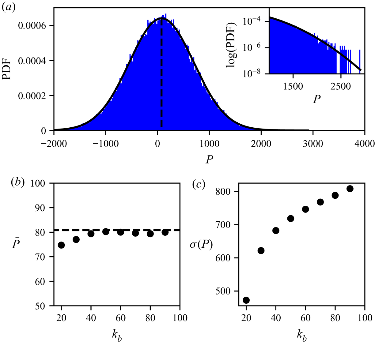
Figure 2. (a) Histogram of stationary time series  $P(t)$ evaluated over $256 T_0$, fitted with a Gaussian distribution of the same mean and standard deviation (solid line) for reference. Inset: tail of the distribution in logarithmic scale. (b) Mean $\bar {P}$ and (c) standard deviation $\sigma (P)$, evaluated for different $k_b$. The dissipation-based estimate of $P_d$ is indicated in both (a) and (b) by a dashed line.
We next examine the relation between  $\sigma (P)$ and nonlinearity level measured by $\bar {P}$, with $\sigma (P)$ as a function of $\bar {P}$ plotted in figure 3. The result shows a power-law relation over two decades given by $\sigma (P) \sim \bar {P}^{0.8 \pm 0.05}$. Furthermore, we include in figure 3 the standard deviation of the exact-resonant contributions to energy flux, $\sigma (P_{\varOmega =0})$, with $P_{\varOmega =0}$ calculated by the decomposition method presented in § 2. We observe a similar power-law relation between $\sigma (P_{\varOmega =0})$ and $\sigma (P)$, but with the value of $\sigma (P_{\varOmega =0})$ $O(10)$ times smaller than $\sigma (P)$ consistently for each nonlinearity level. This indicates that the large fluctuations in $P(t)$ are generated mainly due to quasi-resonant interactions.

Figure 3. Dependence of  $\sigma (P)$ (blue circles) and $\sigma (P_{\varOmega =0})$ (red squares) on $\bar {P}$, with the best fits indicated by dashed lines.
A more detailed study about the contributions of exact- and quasi-resonances to  $\bar {P}$ and $\sigma (P)$ can be conducted by looking into the components of $P_\varOmega$ for varying values of $\varOmega$. In figures 4(a) and 4(b), we plot $\bar {P}_\varOmega$ and $\sigma (P_\varOmega )$ for $\varOmega \in [0,30]$ at four different levels of nonlinearity. We note that $\varOmega$ can take only even integer values for the dispersion relation $\omega _k=k^2$ on a periodic domain of $2{\rm \pi} \times 2{\rm \pi}$. The general trends in figures 4(a) and 4(b) show that $\bar {P}_\varOmega$ decreases, but $\sigma (P_\varOmega )$ increases with the increase of $\varOmega$. This corresponds to a physical picture that as the interactions become more ‘quasi’ (i.e. frequency mismatch $\varOmega$ becomes larger), they contribute less to the mean flux but may contribute more to the fluctuations of the flux. We also emphasize here that while we always have $\sum _\varOmega \bar {P}_\varOmega = \bar {P}$, the quantity $\sum _\varOmega \sigma ^2(P_\varOmega )$ is in general not equal to $\sigma ^2(P)$ because the $P_\varOmega (t)$ with different $\varOmega$ are not independent. Nevertheless, figure 4(b) in conjunction with figure 3 is sufficient to support the dominance of quasi-resonances in generating the large fluctuations in $P(t)$.

Figure 4. Panel (a) shows  $\bar {P}_\varOmega$, and (b) shows $\sigma (P_\varOmega )$, as functions of $\varOmega$, for four levels of nonlinearity with $\bar {P}=81.9$ (blue circles), $\bar {P}=61.0$ (red squares), $\bar {P}=42.8$ (green triangles) and $\bar {P}=20.0$ (purple triangles). (c) Nonlinear broadening $\varGamma$ as a function of $\bar {P}$; (d) number of quartet interactions $\mathcal {N}_{\varOmega }$ for different $\varOmega$. Panels (e) and ( f) are similar to (a) and (b), but plotted for normalized flux $Q_n$. The computations to generate these results are conducted for $k_b=23$ to reduce the computational cost associated with the number of involved quartets.
We conclude this section by summarizing two additional important results regarding  $P_\varOmega$. First, the decomposition in terms of $\varOmega$ enables a direct measure of nonlinear broadening by considering quantitatively the contribution of quasi-resonances to the total energy flux. To demonstrate this, we define a measure of nonlinear broadening $\varGamma \equiv \min \{\varOmega |\bar {P}_{\varOmega }< \alpha \bar {P}_{\varOmega =0} \}$, which is plotted in figure 4(c) for $\alpha =0.1$. While this choice of $\alpha$ can be varied, $\varGamma$ clearly quantifies the nonlinear broadening by measuring the width of $\bar {P}_{\varOmega }$ in $\varOmega$, showing that nonlinear broadening increases with $\bar {P}$. Second, the fluctuations seen in figures 4(a) and 4(b) can be removed by considering the normalized flux $Q_\varOmega (t)=P_\varOmega (t)/\mathcal {N}_\varOmega$. With $\mathcal {N}_\varOmega$ (figure 4d) counting the number of elements in $\sum _{ \boldsymbol {k}\in \{ \boldsymbol {k}|k< k_b \} } S_{\varOmega, \boldsymbol {k}}$, $Q_\varOmega (t)$ calculates the quartet-averaged flux (over quartets with frequency mismatch $\varOmega$), with both $\overline {Q}_{\varOmega }$ and $\sigma (Q_\varOmega )$ behaving smoothly for the range of $\varOmega$ as shown in figures 4(e) and 4( f).
4.2. Scaling of spectral level with flux
To understand the scaling of spectral level with energy flux, we plot in figure 5 the spectral level  $N$ (see (4.1)) as a function of both $\bar {P}$ and $\bar {P}_{\varOmega =0}$, representing total and exact-resonant flux, respectively. Two salient scalings are observed over the three decades of energy flux. At high nonlinearity level with $\bar {P} \in [30,100]$, we find a scaling approaching $N\sim \bar {P}^{1/3}$ (i.e. $\theta =1/3$ with $\theta$ the scaling exponent defined in § 2), consistent with the kinetic scaling of WTT. At low nonlinearity level with $\bar {P} \in [0.3,3]$, the scaling behaves as $N\sim \bar {P}^{1/2}$ (i.e. $\theta =1/2$), consistent with the dynamic scaling from (2.4). We next discuss the mechanisms underlying these two scalings.

Figure 5. The scaling of inertial-range wave action  $N$ with $\bar {P}$ (blue circles) and $\bar {P}_{\varOmega =0}$ (red triangles). The dynamic scaling $\theta =1/2$ and kinetic scaling $\theta =1/3$ are indicated by dashed lines.
For high nonlinearity, we see in figure 5 that we have  $\bar {P} \gg \bar {P}_{\varOmega =0}$, consistent with observations in figure 4(a), indicating that quasi-resonances dominate the dynamics in this regime. This suggests that the kinetic scaling, developed from the WKE in the kinetic limit (infinite domain and small nonlinearity), is realized at relatively high nonlinearity in a finite domain as quasi-resonances overcome the discreteness. This physical picture is consistent with the results of Annenkov & Shrira (Reference Annenkov and Shrira2006), L'vov & Nazarenko (Reference L'vov and Nazarenko2010), Nazarenko (Reference Nazarenko2011) and Pistone, Onorato & Chibbaro (Reference Pistone, Onorato and Chibbaro2018), which all suggest a kinetic wave turbulence regime dominated by quasi-resonance in a finite domain. In addition, recent mathematical justifications of the WKE (Buckmaster et al. Reference Buckmaster, Germain, Hani and Shatah2021; Deng & Hani Reference Deng and Hani2021a,Reference Deng and Hanib) show that the kinetic limit should be taken according to particular scaling laws between the domain size and nonlinearity level, i.e. retaining the quasi-resonances as the large box limit is taken. More specifically, the quasi-resonances are the ones responsible for the emergence of the kinetic equation in the large box limit (Deng & Hani Reference Deng and Hani2021a). However, it should be noted that these mathematical works describe the initial evolution only up to the kinetic time scale, and are not necessarily relevant to the stationary state that we study here. In addition, the mathematical works are developed for the NLSE (which is slightly different from (2.1)) and sometimes require a dimension $d\ge 3$ (Deng & Hani Reference Deng and Hani2021a).
For low nonlinearity,  $\bar {P}\approx \bar {P}_{\varOmega =0}$ (as shown in figure 5) due to the elimination of quasi-resonant contributions to $\bar {P}$, which has been observed previously in Hrabski & Pan (Reference Hrabski and Pan2020). This is because the nonlinear broadening is not sufficient to overcome the discreteness of wavenumber in a finite domain. In this regime, kinetic wave turbulence is not supported (due to the lack of quasi-resonances), and the remaining exact-resonances (on a discrete manifold) lead to a dynamic scaling that can be derived from (2.4). In addition, the dispersion relation $\omega _k=k^2$ is important for the realization of dynamic scaling because otherwise a frozen turbulence (Pushkarev & Zakharov Reference Pushkarev and Zakharov2000) behaviour may be expected at low nonlinearity. For $\omega _k=k^2$, it has been proven (in the context of the NLSE) that for $N\rightarrow 0$, the dynamics at high wavenumbers is described by a continuous resonant equation (Faou et al. Reference Faou, Germain and Hani2016), i.e. the system behaves like a system of continuous wavenumber so that an energy cascade can be expected. In other words, the exact resonances on the discrete manifold determined by $\omega _k=k^2$ are sufficient to support an energy cascade.
In retrospect to figure 1(b), we note finally that the kinetic scaling regime at high nonlinearity is associated with a spectral slope  $\gamma$ that is steeper than the WTT solution $\gamma _0$. This behaviour is also observed in simulations of the MMT equation (in one dimension with a different dispersion relation) by Chibbaro et al. (Reference Chibbaro, De Lillo and Onorato2017). Further investigations on this problem (as well as the result of $\gamma =\gamma _0$ in the dynamic scaling range) are warranted. Here, we remark simply that in order for $\gamma =\gamma _0$ at high nonlinearity, one requires the solution of the kinetic equation (i.e. the Kolmogorov–Zakharov spectrum) to be valid, which is a much stronger requirement than the kinetic scaling.
4.3. Investigation on the closure model
In this subsection, we use our numerical data to study the WTT closure model, in particular the magnitude and functional form of  $f(\varOmega )$. We perform this study for the nonlinearity levels associated with the kinetic scaling of $\bar {P}$, i.e. in the kinetic wave turbulence regime. The function $f(\varOmega )$ in the WTT closure model (as summarized in § 2) is developed for this regime under a discrete setting before the large box limit is taken, and it is this form that we will study with our numerical data. Theoretically, one expects $f(\varOmega )$ to take the form of either a sinc-like function (Janssen Reference Janssen2003; Nazarenko Reference Nazarenko2011) or $\epsilon /(\varOmega ^2+\epsilon ^2)$ (Zakharov et al. Reference Zakharov, L'vov and Falkovich2012), with $\int _\varOmega f(\varOmega )\,\textrm {d}\varOmega \sim O(1)$ since both forms are generalized delta functions. The numerical evaluation of $f(\varOmega )$ will be performed at: (i) an individual quartet level using (2.6); (ii) a family of quartets level using (2.6) in an average manner that will be introduced shortly; and (iii) an inter-scale energy flux level using (2.7). The general procedure is to compute $f(\varOmega )$ from (2.6) and (2.7), with all other terms determined from the numerical data. To distinguish these computations, we denote the numerically obtained $f(\varOmega )$ from the three levels respectively as $f_Q(\varOmega )$, $f_F(\varOmega )$ and $f_P(\varOmega )$.
Figure 6 shows  $f_Q(\varOmega )$ evaluated for $O(50)$ quartets with $\varOmega \in [0,30]$, and with average quantities in (2.6) evaluated over a time window $T_w=256 T_0$. It is clear that no obvious functional pattern can be found for $f_Q(\varOmega )$ (i.e. with different values of $f_Q(\varOmega )$ obtained for the same $\varOmega$). This indicates that the WTT closure for fourth-order correlators cannot be used to describe the behaviour of a single quartet (regardless of its associated frequency mismatch $\varOmega$) in the chosen finite time interval $T_w$. In other words, within $T_w$ (which is long enough to resolve low-order statistics), the contributions of individual quartets to the energy cascade are not described by the WTT closure model. On the other hand, it is not clear from the current results whether there exists a sufficiently long time interval such that we can observe convergent behaviour of fourth-order correlators, and whether the convergent behaviour is described by WTT. To find a definite answer to this question, longer simulations are needed, which will be a topic of future work.

Figure 6. The function  $f_Q(\varOmega )$ evaluated for $O(50)$ selected quartets (with three quartets for each $\varOmega$) with $T_w = 256 T_0$, for the highest nonlinearity level with $\bar {P}=81.9$.
To consider the average behaviour of a family of quartets, we use a technique similar to that of Annenkov & Shrira (Reference Annenkov and Shrira2006) to create a cluster of modes around each of the four modes of an exact-resonant quartet. Specifically, for an exact quartet ( $\boldsymbol {k}_0^e$, $\boldsymbol {k}_1^e$, $\boldsymbol {k}_2^e$, $\boldsymbol {k}_3^e$), we construct a family of quartets ( $\boldsymbol {l}_0$, $\boldsymbol {l}_1$, $\boldsymbol {l}_2$, $\boldsymbol {l}_3$) at its vicinity by choosing all $\boldsymbol {l}_i$ with $|\boldsymbol {l}_i- \boldsymbol {k}_i^e|\le 4$ for $i=0,1,2,3$. We then evaluate $f_F(\varOmega )$ from (2.6) by summing over those quartets ( $\boldsymbol {l}_0$, $\boldsymbol {l}_1$, $\boldsymbol {l}_2$, $\boldsymbol {l}_3$) with frequency mismatch $\varOmega$ on both sides of the equation. Under this evaluation, $f_F(\varOmega )$ reflects the closure behaviour averaged over $O(10^3)$ quartets. Figure 7 shows $f_F(\varOmega )$ computed from three representative families of quartets, defined via exact quartets ( $\boldsymbol {k}_0^e$, $\boldsymbol {k}_1^e$, $\boldsymbol {k}_2^e$, $\boldsymbol {k}_3^e$). We see that $f_F(\varOmega )$ is somewhat inversely proportional to $\varOmega$ superposed with many fluctuations. While the general trend of $f_F(\varOmega )$ seems consistent for different families, the details (e.g. the value of $f_F(0)$ as well as the fluctuation patterns) vary considerably across different families.

Figure 7. The function  $f_F(\varOmega )$ for three representative families of quartets defined by $\boldsymbol {k}_0^e=(-2,8)$, $\boldsymbol {k}_1^e=(-10,0)$, $\boldsymbol {k}_2^e=(14+4j,-8-4j)$ and $\boldsymbol {k}_3^e=(6+4j,-16-4j)$, for $j=0$ (blue circles), $j=1$ (red squares) and $j=2$ (green triangles). The evaluation is for the highest nonlinearity case of $\bar {P}=81.9$ with $T_w = 256 T_0$.
Finally, we examine the closure behaviour considering the average over an enormous number of quartets, chosen as all quartets contributing to the energy flux across  $k_b=23$. Under such a consideration, both sides of (2.7) are subject to summation over $O(10^9)$ elements in $\sum _{ \boldsymbol {k}\in \{ \boldsymbol {k}|k< k_b \} } S_{\varOmega, \boldsymbol {k}}$ for each $\varOmega$ (see figure 4d). The numerically resolved $f_P(\varOmega )$ is plotted in figure 8 at several different nonlinearity levels. We remark that these results are convergent in the sense that they are not sensitive to the length of the time window $T_w$ (we have checked that using $T_w/4$ as the time window leads to the same result). It is clear that under this level of average, $\int _\varOmega f(\varOmega )\,\textrm {d}\varOmega \sim O(1)$ consistent with WTT (we do not expect $\int _\varOmega f(\varOmega )\, \textrm {d}\varOmega$ to be exactly 1 unless we can reach the kinetic limit numerically). To quantify the profile of $f_P(\varOmega )$, we use a least-squares method to fit the data to a general functional form of $f_P(\varOmega )=C/(\rho + \varOmega ^{\beta })$, where $\rho$ is needed as a desingularization factor for $f_P(0)$. These fittings, as shown in figure 8, agree with all data points remarkably well, with $C=[1.06,0.982,0.875]$, $\rho =[6.176,3.44,2.26]$ and $\beta =[1.35,1.47,1.52]$ from high to low nonlinearity level. Instead of a sinc-like function (which involves either negative values or oscillatory behaviour, with neither observed), the functional form of $f_P(\varOmega )$ is somewhat closer to the WTT form of $\epsilon /(\varOmega ^2+\epsilon ^2)$, but with different exponents $\beta$. This is probably why Pan & Yue (Reference Pan and Yue2017) find that the kinetic equation employing this WTT form of generalized delta function produces physically reasonable results in terms of the spectral slope and energy flux for capillary waves.

Figure 8. The function  $f_P(\varOmega )$ evaluated by (2.7) with $k_b=23$ and $T_w = 256 T_0$, for different nonlinearity levels, with $\bar {P}=81.9$ (blue circles), $\bar {P}=42.8$ (red squares) and $\bar {P}=28.0$ (green triangles). Fits to the data of the form $f(\varOmega )=C/(\rho + \varOmega ^{\beta })$ are indicated by the dashed lines.
5. Conclusion and discussions
In this paper, we study numerically the properties of inter-scale energy flux  $P$ for wave turbulence in the context of the 2-D MMT equation. Unlike previous evaluations of $P$ based on energy input or dissipation rate, our formulation of $P$ computes the exact instantaneous energy flux across arbitrary scale $k_b$ directly from the nonlinear terms in the MMT equation, and allows a quartet-level decomposition of $P$ into $P_\varOmega$ according to the frequency mismatch $\varOmega$ of the quartets. Our results show that the energy flux $P$ across any scale in the inertial range closely follows a Gaussian distribution, with the mean value $\bar {P}$ almost a constant for any $k_b$, and standard deviation $\sigma (P)$ increasing with $k_b$. In addition, values of $\sigma (P)$ are generally several orders of magnitude larger than $\bar {P}$, mainly due to the contributions to $\sigma (P)$ from quasi-resonances, i.e. $P_{\varOmega >0}$. The decomposition of $P$ into $P_\varOmega$ also allows an alternative but more direct measure of nonlinear broadening by quantitatively considering the contribution of quasi-resonances to the mean energy flux. We further study the scaling of spectral level $N$ with the energy flux and find that $N\sim \bar {P}^{1/3}$ (consistent with the kinetic scaling) at high nonlinearity, and $N\sim \bar {P}^{1/2}$ (dynamic scaling) at low nonlinearity. The former and latter are due to the dominance of the quasi-resonant and exact-resonant contributions to $\bar {P}$, respectively. Finally, our numerical study on the wave turbulence closure model shows that the fourth-order correlator evaluated over a finite time window is in disagreement with the description by the theoretical closure on a single quartet level. When considering the average over all quartets contributing to the inter-scale energy flux (over $O(10^9)$ quartets for each $\varOmega$), a behaviour more consistent with the theoretical closure is observed, but with the broadening function exhibiting $1/\varOmega ^\beta$ (with $\beta$ between $1.3$ and $1.6$), different from the forms derived in WTT.
While this work sheds new light on the physics of wave turbulence, more unanswered questions about wave turbulence, especially regarding the closure model, are raised. The closure model is a subject that has received insufficient attention from a numerical perspective, especially in terms of analysis utilizing data generated directly from the primitive dynamic equation. The few exceptions to this (e.g. Majda et al. Reference Majda, McLaughlin and Tabak1997; Annenkov & Shrira Reference Annenkov and Shrira2006; Sheffield & Rumpf Reference Sheffield and Rumpf2017) have not considered the detailed functional form and magnitude of  $f(\varOmega )$, as studied in this work. Therefore, the authors consider the primary importance of this work as to provide a methodology such that many open questions in wave turbulence can be studied directly using vast numerical data. Within the presented results, for example, the function $f_Q(\varOmega )$ in figure 6 is still sensitive to the time window $T_w$ used for averaging quantities in (2.6) for an individual quartet. It is not clear whether a convergent behaviour (close to the quartet-averaged result $f_P(\varOmega )$) can be found if a time average over an extremely long time window is performed. In addition, will the smooth behaviour associated with function $Q_\varOmega$ in figures 4(e) and 4( f) be preserved in different domain geometries (e.g. an irrational torus as in Hrabski et al. Reference Hrabski, Pan, Staffilani and Wilson2021) where the normalization factor $\mathcal {N}_\varOmega$ varies substantially? Last but not least, are we able to explore the kinetic limit in numerical simulations by varying both domain size and nonlinearity level? If this is possible, will we find more consistent behaviour for $f_F(\varOmega )$ for families centred on different quartets, and will all these functions eventually converge to a delta function?
These questions can be explored in greater detail with increasing computational resources, and it is certainly not unreasonable to think about studying wave turbulence with ‘exascale computing’, an area under development for hydrodynamic turbulence (e.g. Yeung & Ravikumar Reference Yeung and Ravikumar2020). For wave turbulence, these resources may be better utilized in conjunction with an understanding of WTT, rather than simply boosting the resolution of simulations. It might also be beneficial to revisit the one-dimensional MMT equation, where some of these questions can be investigated with a reduced computational cost but with the new techniques developed here. In doing this, we may also hope to settle the dispute between the WTT and MMT closure models that has been haunting the field for more than 20 years.
Acknowledgements
Any opinions, findings, and conclusions or recommendations expressed in this material are those of the authors and do not necessarily reflect the views of the National Science Foundation.
Funding
This material is based upon work supported by the National Science Foundation Graduate Research Fellowship under Grant no. DGE 1841052. This work used the Extreme Science and Engineering Discovery Environment (XSEDE), which is supported by National Science Foundation grant no. ACI-1548562. Computation was performed on XSEDE Bridges-2 at the Pittsburgh Supercomputing Center through allocation PHY200041. This research was supported in part through computational resources and services provided by Advanced Research Computing (ARC), a division of Information and Technology Services (ITS) at the University of Michigan, Ann Arbor.
Declaration of interests
The authors report no conflict of interest.
Appendix
In figure 9, we provide the relationships between nonlinearity  $\varepsilon$ and wave action measure $N$, and between $\varepsilon$ and mean flux $\bar {P}$. We observe monotonic scaling relationships in both cases.

Figure 9. The relationships of (a)  $\varepsilon$ with $N$, and (b) $\varepsilon$ with $\bar {P}$.


 Open access