


1. Introduction
1.1. Background and objectives
Glaciers are shrinking globally due to warming temperatures (e.g. Pörtner and others, Reference Pörtner2019; Hugonnet and others, Reference Hugonnet2021), and the rate of this ice volume loss is forecast to increase over the course of the 21st century (e.g. Radić and Hock, Reference Radić and Hock2011; Radić and others, Reference Radić2014). Melting glaciers release water from terrestrial storage and contribute to sea level rise. Tidewater glaciers release this meltwater directly into the ocean, while land or lake-terminating glaciers release it into terrestrial drainage systems. The routing of glacier meltwater through these terrestrial drainage systems may constitute an important proportion of the local water budget (Saberi and others, Reference Saberi2019; Kraaijenbrink and others, Reference Kraaijenbrink, Stigter, Yao and Immerzeel2021) and contribute to geohazards such as glacial lake outburst floods (e.g. Richardson and Reynolds, Reference Richardson and Reynolds2000; Cook and others, Reference Cook, Kougkoulos, Edwards, Dortch and Hoffmann2016; Carrivick and Tweed, Reference Carrivick and Tweed2016; Veh and others, Reference Veh, Korup and Walz2020).
The future contribution of glaciers to streamflow in a warming climate can be grouped into three categories: (i) “stable” glaciers, with a mass balance approximately in steady state, (ii) glaciers with a negative mass balance and increasing meltwater output, and (iii) glaciers with a negative mass balance and decreasing meltwater output (e.g. Jansson and others, Reference Jansson, Hock and Schneider2003; Barnett and others, Reference Barnett, Adam and Lettenmaier2005; Huss and Hock, Reference Huss and Hock2018; Pörtner and others, Reference Pörtner2019). Glaciers with a positive mass balance may also exist (Miles and others, Reference Miles2021), but in a warming climate can generally be neglected on a regional scale. At any given glacier, an initial temperature rise and increase in ablation (negative mass balance) will increase the glacier's meltwater output. The glacier will then shrink in response to the negative surface mass balance, until its reduced area/volume is no longer able to sustain the same meltwater output. The glacier's contribution to streamflow will then shrink over time until the glacier reaches a new steady state or disappears entirely. The turning point of the meltwater output curve is known as ‘peak water’.
Ice volume loss supplies water to streams, thereby modulating their discharge. Where isolating the contribution to streamflow of glacier volume loss to streamflow is possible, which requires an understanding of the other components of the local water balance, proglacial stream discharge may be used to study changes in glacial water storage within the drainage basin (e.g. Hock and others, Reference Hock, Jansson and Braun2005; Sicart and others, Reference Sicart, Ribstein, Francou, Pouyaud and Condom2007; Konz and Seibert, Reference Konz and Seibert2010; O'Neel and others, Reference O'Neel, Hood, Arendt and Sass2014; Beamer and others, Reference Beamer, Hill, Arendt and Liston2016). River discharge may be measured from a single point, whereas accurate measurements of glacier mass balance require a full 2D field of elevation-change measurements.
Glacier volume loss and time-integrated river discharge are only directly equal where a river is sourced exclusively from glacier ice–for instance, a proglacial stream at its source. In most cases, a portion of glacial meltwater is lost to temporary terrestrial storage (e.g. lakes, groundwater) or evapotranspiration and supplemented by precipitation. The relative proportions of the glacial, terrestrial water storage, precipitation, and evapotranspiration contributions vary widely (e.g. Beamer and others, Reference Beamer, Hill, Arendt and Liston2016; Carrivick and others, Reference Carrivick, Heckmann, Fischer and Davies2019). For example, the contribution of glacier volume loss to streamflow can be as high as 60% in a 34% glacierised catchment in the proximal drainages of Ecuadorian volcano Chimborazo (Saberi and others, Reference Saberi2019). However, at the mouth of the Amazon, thousands of kilometers downstream, the glacial contribution to streamflow is negligible (Gupta, Reference Gupta2008).
We hypothesize that the rate of Patagonian glacier volume loss has accelerated over the past two decades, particularly through a lengthening of the melt season. To investigate this, we combine discharge measurements of Patagonian rivers with precipitation, evapotranspiration, and lake-volume data to calculate a monthly-resolution hydrological balance for 11 sub-basins.
1.2. Study area
The Northern and Southern Patagonian Icefields (NPI and SPI) are the Southern Hemisphere's largest ice masses outside of Antarctica, with a combined glacierised area of around 17,500 km2 (Davies and Glasser, Reference Davies and Glasser2012). Tidewater glaciers on the western margin of the icefields terminate directly into Pacific fjords, while lake-terminating glaciers on the eastern margin of the icefields drain into large proglacial lakes. These proglacial lakes are connected to the Pacific and Atlantic Oceans via a proglacial drainage network. Four main rivers drain this eastern margin of the icefields, from North to South: Río Baker (drains the NPI into the Pacific), Río Pascua and Río Serrano (drain the SPI into the Pacific) and Río Santa Cruz (drains the SPI into the Atlantic). All of these rivers and a number of tributaries are gauged, with monthly or shorter interval discharge measurements (Figs. 1 and 2).
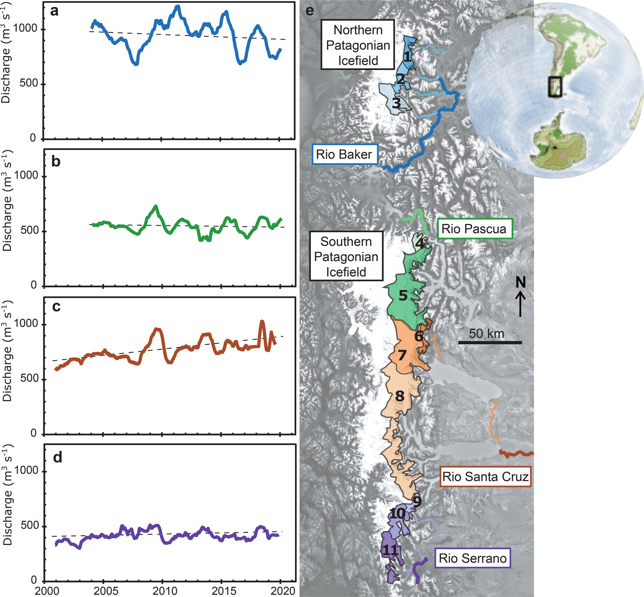
Fig. 1. Map of the Patagonian Icefields (e), together with the four main fluvial drainage networks: Río Baker (a), Río Pascua (b), Río Santa Cruz (c) and Río Serrano (d). The discharge of each river over the 21st century is shown in the subpanels (a–d).
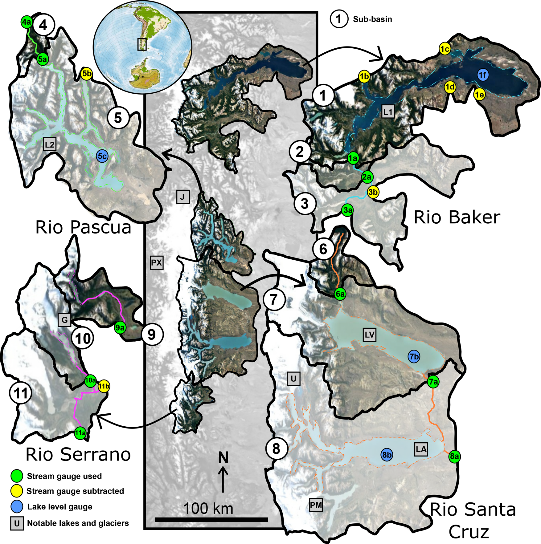
Fig. 2. Gauging stations used in this study. Gauges labeled in yellow were subtracted from the respective downstream green gauge to reduce the non-glacierised contributing area. Specific information about each gauge is given in Table 1. Sub-basins in each river basin are shown with different levels of transparency for visibility. L1 = Lago General Carrera/Buenos Aires; L2 = Lago O'Higgins/San Martín; LV = Lago Viedma; LA = Lago Argentino; J = Glaciar Jorge Montt; PX = Glaciar Pio XI; U = Glaciar Upsala; PM = Glaciar Perito Moreno; G = Glaciar Grey.
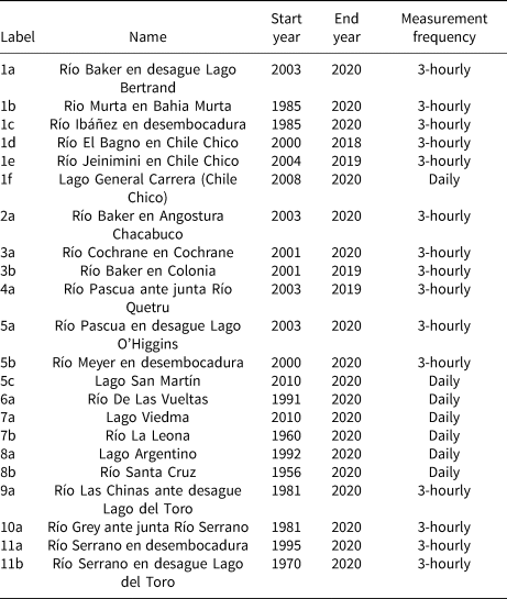
Table 1. Details of all stream and lake gauges used in this study
.
The Patagonian Icefields are retreating rapidly–with the NPI and SPI having lost 100 and 500 km3 respectively since their late-Holocene maximum (Glasser and others, Reference Glasser2011), out of a total present-day volume of 4, 756 ± 923 km3 (Millan and others, Reference Millan2019). The Icefields’ current rates of ice volume loss, at around 20 km3 a−1 (Malz and others, Reference Malz2018; Abdel Jaber and others, Reference Abdel Jaber, Rott, Floricioiu, Wuite and Miranda2019), are the highest on record (Rignot and others, Reference Rignot, Rivera and Casassa2003; Malz and others, Reference Malz2018; Zemp and others, Reference Zemp2019; Hugonnet and others, Reference Hugonnet2021), and their specific mass change (thinning) rate is the highest of any glacierised region on Earth (Zemp and others, Reference Zemp2019). This rapid volume loss is not evenly distributed: some glaciers have experienced extremely rapid retreat (e.g. Upsala, Jorge Montt: Saito and others, Reference Sakakibara, Sugiyama, Sawagaki, Marinsek and Skvarca2013; Minowa and others, Reference Minowa, Schaefer, Sugiyama, Sakakibara and Skvarca2021), while others have remained stable or advanced (e.g. Perito Moreno, Pio XI: Skvarca and Naruse, Reference Skvarca and Naruse1997; Rivera and Casassa, Reference Rivera and Casassa1999; Guerrido and others, Reference Guerrido, Villalba and Rojas2014; Hata and Sugiyama, Reference Hata and Sugiyama2021).
Volume loss of the Patagonian Icefields has been examined across timescales: on the long term through geomorphological mapping and cosmogenic nuclide dating, and on the short term by a range of remote-sensing techniques. Satellite assessments of ice loss include satellite gravimetry (Chen and others, Reference Chen, Wilson, Tapley, Blankenship and Ivins2007; Jacob and others, Reference Jacob, Wahr, Pfeffer and Swenson2012; Li and others, Reference Li, Chen, Ni, Tang and Hu2019; Richter and others, Reference Richter2019) and various forms of satellite altimetry (Rignot and others, Reference Rignot, Rivera and Casassa2003; Willis and others, Reference Willis, Melkonian, Pritchard and Rivera2012; Foresta and others, Reference Foresta2018; Malz and others, Reference Malz2018; Dussaillant and others, Reference Dussaillant2019; Abdel Jaber and others, Reference Abdel Jaber, Rott, Floricioiu, Wuite and Miranda2019; Hugonnet and others, Reference Hugonnet2021). Remotely sensed observations may have limited temporal and spatial resolution or require in-situ calibration, and so can be complemented by field measurements. However, field-based assessments of Patagonian glacier volume loss are sparse. Increased discharge has been observed on rivers draining the SPI (Pasquini and others, Reference Pasquini, Cosentino and Depetris2021), but this has not been used to directly calculate changes in the rate of glacier volume loss.
2. Methods
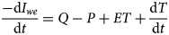
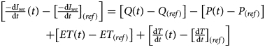
We process runoff data for Patagonian proglacial rivers to recover a ground-based estimate of the rate of glacier volume loss. This approach is based on the conservation of water within a glacierised basin: a balance exists between the water entering the system (precipitation), exiting the system (evapotranspiration plus river discharge), and stored within the system (groundwater, lacustrine, or glacial water storage). We write an equation for the conservation of water within a given glacierised basin with the change in water storage equal to the water inputs minus the water outputs:

with I we being the water storage in glacial ice (in m3 water equivalent), T being terrestrial water storage (in m3), P being precipitation (in m3 s−1), ET being evapotranspiration (in m3 s−1), and Q being total river discharge (in m3 s−1). The total change in water storage is given by the left-hand terms in this equation, water inputs are given by precipitation P, and water outputs are given by evapotranspiration and runoff [ET + Q].
We wish to evaluate the rate of glacier volume loss, equal to the negative change in glacier water storage over time. We therefore rearrange equation (1) to isolate the rate of glacier volume loss term:
Instead of attempting to close the full water balance, we write each term as an anomaly, subtracting the average value of that term during a reference period from any given (transient) measurement. The calculation of a relative glacier volume loss (rGVL) anomaly only requires relative changes in total discharge, precipitation, rates of terrestrial water storage change, and evapotranspiration instead of their absolute magnitudes. In the case of discharge data, this adds further robustness to our calculation, because uncertainties associated with the rating curve affect relative changes in discharge less than they impact the calculation of the absolute discharge magnitude (Shiklomanov and others, Reference Shiklomanov2006; Kiang and others, Reference Kiang2018). By using an anomaly, we can also reduce the effects of overestimating or underestimating the rate of glacier volume loss due to missing streamflow contributions. This is because subtracting a reference amount from each measurement is the equivalent of approximating any missing terms as time-invariant over other time periods, instead of the less realistic scenario of treating them as zero-magnitude. We define a reference period of 2000-2005, a period with data for all discharge contributions and across all sub-basins (except lake level gauges). While some discharge gauges have substantially longer records (e.g. 1956-present for the Río Santa Cruz), widespread precipitation and evapotranspiration data is not available prior to 2000, and we prefer selecting a common reference period for all datasets. Each anomaly is calculated as:
with (t) representing the given time of each measurement, and (ref) indicating that the average of the reference period (2000–2005) was taken. Changing equation (3) to an anomaly notation (δ) gives:

This anomaly in rate of water equivalent glacier volume loss may be converted into a rGVL anomaly by correcting for ice density δ[ − dI/dt]:
with ρ I and ρ W being the densities of ice and water, respectively (in kg m−3).
2.1. River discharge
We obtain river discharge data from a series of gauging stations in Chile and Argentina. These gauging stations are in the drainage basins of Río Baker, Río Pascua, Río Santa Cruz, and Río Serrano (Fig. 1). To improve the spatial resolution of our rGVL anomaly, we subdivide each drainage into the smallest available units based on the distribution of gauging stations. Where gauging stations are available on non-glacierised tributaries of these rivers, we subtract their discharge values from the flow of the main channel, thereby effectively maximizing the percentage glacierised area considered within catchments and the fraction of streamflow derived from glacier volume loss (Fig. 2 and Table 1). Specifically, we subtract discharge at gauging stations 1b, 1c, 1d, and 1e from 1a; 3b from 3a; 5b from 5a; and 11b from 11a (see Fig. 2 and Table 1). We measure and subdivide drainage basins using TopoToolbox in Matlab (Schwanghart and Scherler, Reference Schwanghart and Scherler2014) based on the 30 m resolution SRTM DEM (Farr and others, Reference Farr2007). Using this workflow, we divide the Río Baker, Río Santa Cruz, and Río Serrano basins into three sub-basins, and the Río Pascua basin into two sub-basins (Fig. 2). Each sub-basin drains a distinct sector of the NPI or SPI, spatially integrating the glacier volume loss of all glaciers within the sub-basin area.
We acquire discharge data from all gauging stations at the highest available temporal resolution (Table 1). We then average all daily resolution datasets to a monthly resolution for further analysis. All data is available in public portals: http://bdhi.hidricosargentina.gob.ar/ for Argentina and https://snia.mop.gob.cl/BNAConsultas/reportes for Chile. Discharge data are provided without any uncertainty metric, so we assign 5% uncertainty to mean annual discharge measurements and 15% uncertainty to mean monthly discharge measurements based on an evaluation of high-latitude rivers in Russia (Shiklomanov and others, Reference Shiklomanov2006). We note that the data also included no information about the exact gauging methods or rating curves used, so this information could not be evaluated.
2.2. Precipitation
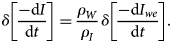
Too few precipitation gauges are present in Southern Patagonia to use instrumental data alone, so we use the remotely sensed Integrated Multi-satellitE Retrievals for GPM (GPM IMERG) precipitation dataset. This algorithm processes precipitation data from both the GPM and earlier TRMM satellites, and incorporates additional information from a global network of stream gauges. This dataset is provided at half-hourly temporal resolution and 0.1 degree pixel spatial resolution ( 10 km)– covering the period from June 2000 to present. We use a Google Earth Engine script to calculate an average precipitation value for each sub-basin, and then download precipitation data in monthly-averaged time steps. This should be a conservative uncertainty quantification, also because we further apply a correction factor to GPM IMERG-derived precipitation data based on differences we calculated (using an outlier-robust iteratively re-weighted least-squares algorithm) between GPM IMERG values and measurements from 11 precipitation gauges located around Southern Patagonia (Fig. 3). We calculate a precipitation correction factor of 0.44 based on the comparison between GPM IMERG and 11 local precipitation gauges. Despite an absolute difference between the instrumental and remotely sensed datasets of a factor of 2, the two time series are highly correlated (mean correlation coefficient of 0.81) and exhibit very similar anomalies (−19% and −16% for the period 2016–2020 relative to 2000–2005 for the instrumental data and GPM IMERG respectively - see a breakdown for each gauge in supplementary section S1). For our error analysis, we used a 22% uncertainty bound, which is the upper limit of the 7 to 22% error range previously found for GPM IMERG (NASA IMERG technical documentation; Tang and others, Reference Tang2020). We consider the upper bound of the error range to be the most appropriate as Patagonia exhibits very high precipitation gradients, and very few precipitation gauges on the high-precipitation western regions (Garreaud and others, Reference Garreaud, Lopez, Minvielle and Rojas2012; Lenaerts and others, Reference Lenaerts2014).
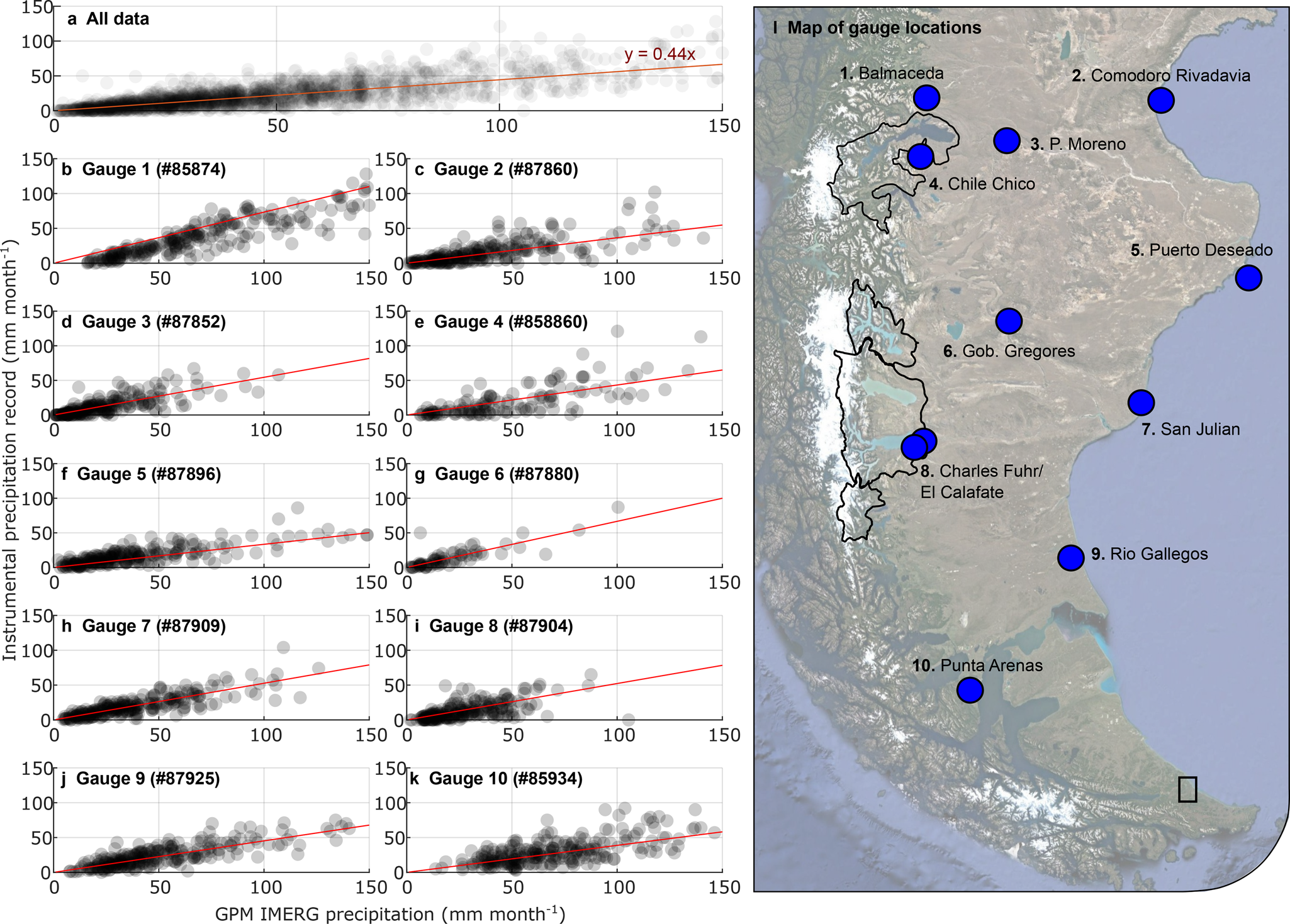
Fig. 3. Comparison between remotely sensed precipitation values and instrumental data, used to build a regional correction factor for precipitation in Southern Patagonia. (a) shows the data for all precipitation gauges, (b)–(k) show the data for individual gauges along with their weather station numbers, and (l) shows the location of the gauges relative to our study area (highlighted in a darker color). Red lines in (a)–(k) show the linear regression fits to the data, with data available in Table S1.
2.3. Evapotranspiration
We use evapotranspiration data from the Terra Moderate Resolution Imaging Spectroradiometer (MODIS) MOD16A2 dataset. MOD16A2 combines daily re-analysis of meteorological data with MODIS remote-sensing datasets to provide a value for evapotranspiration and latent heat flux. The evapotranspiration values are calculated using the Penman-Monteith equation, using daily mean temperature, wind-speed, relative humidity, and solar radiation (Penman, Reference Penman1948; Monteith, Reference Monteith1965; McNaughton and Jarvis, Reference McNaughton and Jarvis1984). The data are provided at a 500 m pixel spatial resolution and 8-day temporal resolution, which we average into a monthly average evapotranspiration time series for each sub-basin. The MOD16A2 dataset was also successfully used by Alvarez-Garreton and others (Reference Alvarez-Garreton2018) in a recent Chile-wide database of catchment attributes. Patagonian landscapes may exhibit a large range of surface cover types within a single 500 m resolution grid cell, and a range of wind speeds within a single day not captured by the MOD16A2 dataset. Mean error estimates for the MOD16A2 evapotranspiration dataset span 24.1%–24.6% (Running and others, Reference Running, Mu, Zhao and Moreno2019), and so we use an uncertainty of 25% for our uncertainty analysis.
2.4. Terrestrial water storage
A range of terrestrial environments may store water on the short or long term, either drawing water down or releasing it into the local drainage system. For instance, water may be stored in lakes (Sugiyama and others, Reference Sugiyama2016), permafrost (Saito and others, Reference Saito2016; Drewes and others, Reference Drewes, Moreiras and Korup2018), rock glaciers (Selley and others, Reference Selley2019; Schaffer and others, Reference Schaffer, MacDonell, Réveillet, Yáñez and Valois2019), peatlands (Iturraspe and Urciuolo, Reference Iturraspe and Urciuolo2021), and groundwater (Döll and others, Reference Döll, Kaspar and Lehner2003). Two components of our study design facilitate the treatment of terrestrial water storage:
1. We calculate a hydrological anomaly instead of attempting to close the full water balance. Therefore, any terrestrial water storage terms which change sufficiently slowly over time can be neglected, even where their absolute magnitude is non-negligible in the full water balance.
2. We do not study seasonal changes within a given year, and only consider the annual means or the change in individual months across years. Therefore, any seasonal cycle in terrestrial water storage which remains constant across years will not affect our results.
Considering both of these points, any terrestrial water storage system exhibiting low overall change, or high seasonal change and low multiannual change, can be excluded from our calculations. In an ideal scenario, all components would be considered, but this is not possible due to the scale and data limitations of our study area.
Permafrost degradation is an important component of the water balance in some regions, but is only present in restricted high-altitude areas in our study area (Ruiz and others, Reference Ruiz, Beriain, Izagirre, Bockheim and Pedro2015; Saito and others, Reference Saito2016). Previous studies in Patagonia and other glaciated regions suggest that the volume of groundwater change is small relative to the other components over the annual timescales considered (Kane and Yang, Reference Kane and Yang2004; Beamer and others, Reference Beamer, Hill, Arendt and Liston2016; Richter and others, Reference Richter2019). For example, Richter and others (Reference Richter2019) found that including a continental water storage correction term (Döll and others, Reference Döll, Kaspar and Lehner2003) affected their satellite-gravimetry-based estimates of 15-year mean ice mass loss by only 1%, less than the effect of glacio-isostatic adjustment (GIA) or the Antarctic ice sheet mass loss. Richter and others (Reference Richter2019) show that local groundwater exhibits a moderate seasonal cycle and little to no multiannual change (e.g. Richter and others, Reference Richter2019, Figure 2a). Where abundant, rock glacier degradation may contribute to streamflow (Duguay and others, Reference Duguay, Edmunds, Arenson and Wainstein2015; Drewes and others, Reference Drewes, Moreiras and Korup2018; Schaffer and others, Reference Schaffer, MacDonell, Réveillet, Yáñez and Valois2019). A number of rock glaciers are present in Patagonia, but these are sparse relative to the central Andes, cover a very small fraction of each sub-basin, and are mostly <0.05 km2 (Selley and others, Reference Selley2019; Schaffer and others, Reference Schaffer, MacDonell, Réveillet, Yáñez and Valois2019; Zalazar and others, Reference Zalazar2020). A local study in Tierra del Fuego showed that a bog was able to store 35% of a daily precipitation event (Iturraspe and Urciuolo, Reference Iturraspe and Urciuolo2021), but no regional data on wetland water storage is available across Patagonia. Based on this, we exclude permafrost, rock glaciers, groundwater, and wetland water storage from our water balance, reducing the terrestrial water storage to lakewater storage. While existing data and studies of similar locations suggest that these terms are likely a minor component of the hydrological cycle (Kane and Yang, Reference Kane and Yang2004; Beamer and others, Reference Beamer, Hill, Arendt and Liston2016; Drewes and others, Reference Drewes, Moreiras and Korup2018; Schaffer and others, Reference Schaffer, MacDonell, Réveillet, Yáñez and Valois2019; Richter and others, Reference Richter2019; Zalazar and others, Reference Zalazar2020), more detailed studies are necessary to fully quantify their respective contributions in Patagonia. Future studies could include these other terrestrial water storage terms when more is available about them, particularly if attempting to close the full water balance.
Many of the outlet glaciers draining the eastern margin of the Patagonian Icefields terminate in large proglacial lakes. With areas upwards of 1000 km2, small variations in lake-surface elevation may reflect large changes in water storage. We therefore account for changes in water volume within the four largest lakes: Lago Buenos Aires/General Carrera (NPI, 1850 km2), Lago O'Higgins/San Martín (SPI, 1015 km2), Lago Viedma (1090 km2), and Lago Argentino (1470 km2; see Fig. 2). Each of these lakes is gauged, providing daily to sub-daily changes in lake-surface elevation (Fig. 2). We convert each lake surface elevation anomaly into lake volume anomaly by multiplying by lake area, and neglect non-linear volume changes associated with changes in lake surface area. Lake elevation time series have no uncertainty metric, so we assign a conservative 5% uncertainty to all lake-level gauge measurements. We average each dataset into a monthly time series, which also averages out any short-period changes related to lacustrine processes (e.g. 1.5 hour period seiches in Lago Argentino; Richter and others, Reference Richter2016). A number of smaller (<40 km2), ungauged lakes are also present, which are not accounted for in water balance calculations. A 1 m change in surface elevation over one year in the largest of these, Lago Grey, would only be equivalent to a 1 m s−1 change in discharge, which is negligible relative to other contributions. For the four large lakes considered, data from 2000–2005 is unavailable for three of the lake-level gauges, so we use the first two available years of data as the reference period.
The Río Santa Cruz is affected by glacial outburst floods related to the damming of the southern branch of Lago Argentino by Glaciar Perito Moreno, occurring every few years. Once the ice-dam is breached, the southern branch of the lake drains out of the Río Santa Cruz over a timescale of several days, greatly increasing the river's discharge (Pasquini and others, Reference Pasquini, Cosentino and Depetris2021), even though there is no new glacier melt occurring. We use lake-level data from the southern branch of Lago Argentino, Brazo Rico, to track and exclude these flood events from the glacier melt analysis, defining flood events as times when the Brazo Rico lake level lowers by more than 10 cm in a single day.
2.5. Calculation of glacial meltwater anomaly
We preprocess the data as described above to create monthly time series of δQ, δP, δET, and δ[dL/dt], which we use to calculate δ[ − dI we/dt] and δ[ − dI/dt] according to Eqn. 3. We use this monthly time series to create 13 annual time series: one annual average time series across all 12 months, and 12 time series composed of a single month across years. We assume that the uncertainty distributions of each of the contributing time series are normal and independent – i.e., the timeseries’ uncertainty distributions are uncorrelated over time and between time series. This assumption allows us to propagate uncertainties without estimating covariance matrices. Each time series is measured using an entirely independent method, so we do not expect their uncertainties to correlate. We calculate an annual rGVL anomaly (δ[ − dI/dt]) using the annual average time series across all 12 months, and 12 monthly anomalies in rate of glacier volume loss timeseries using the 12 monthly timeseries. We propagate uncertainties from each time series to final ice volume loss estimates.
We integrate the annual rGVL anomaly (δ[ − dI/dt]) over time to create the ice-volume-loss anomaly δ[ − dI/dt]C (in km3). We also normalize the glacier-volume-loss anomalies by glacier area to calculate vertical equivalent ice loss. We convert ice-volume-loss estimates to sea-level-rise equivalent by dividing the water-equivalent ice-volume loss by the global ocean area of 361 million km2, and calculate mean rates of ice loss by dividing by ice surface areas calculated from the Randolph Glacier Inventory v6.0 (Pfeffer and others, Reference Pfeffer2014).
We calculate the temporal average and slope of the rGVL anomaly. The time-averaged rGVL anomaly shows any increase or decrease in ice-volume loss over the 2006–2019 study period relative to 2000–2005 levels, while the slope of the annual rGVL anomaly shows any acceleration or deceleration in ice volume loss over the 2006-2019 study period. We evaluate the significance of changes in ice loss by applying the Mann-Kendall test to the time-integrated rGVL anomaly (δ[ − dI/dt]C) and the annual rGVL anomaly time series (δ[ − dI/dt]).
In summary, we use our monthly-resolution hydrological balance to calculate the rate of change in ice volume as an anomaly over our study period of 2006–2019, relative to a 2000–2005 reference period (Fig. 4). This rate-of-glacier-volume-loss (rGVL) anomaly is equivalent to the rate of change in glacier volume, minus a constant accounting for the rate of change in ice volume over the reference period (Eqns (3)–(5)). Positive rGVL values indicate more rapid ice-volume loss than during the reference period, whereas negative values indicate that ice is being lost less rapidly. The slope of the rGVL anomaly over our 2006–2019 study period (time-averaged second derivative of glacier volume with time) reports whether the rate of glacier volume loss has been accelerating, decelerating, or remaining constant over time. We calculate the rGVL anomaly for whole years and for single months across years to evaluate both the rate and seasonality of glacier volume change (Fig. 7). Finally, we calculate the total time-integrated rGVL anomaly over our study period (Fig. 6) and convert this to sea-level-rise equivalent.
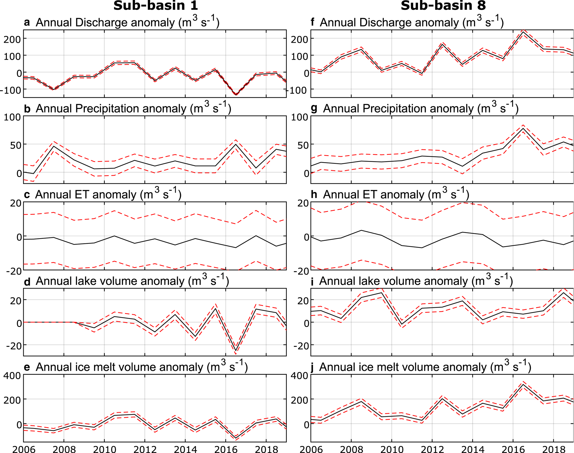
Fig. 4. Magnitude of the discharge, precipitation, evapotranpiration, and lake-volume-change anomalies for sub-basin 1, Lago Buenos Aires/General Carerra (a)–(d), and sub-basin 8, Lago Argentino (e)–(f). The dashed red lines provide the ±1 standard-deviation uncertainty bounds around estimates based on measurements in black lines.
3. Results
3.1. Precipitation, evapotranspiration, and lake level timeseries
The relative importance of the discharge, precipitation, evapotranpiration, and lake-volume-change-rate anomalies to the calculation of the rGVL anomaly (see Eqn (4)) vary across the 11 sub-basins. The discharge anomaly has the largest magnitude in 82% of sub-basins (e.g. Fig. 4). The sign of the time-averaged discharge anomaly varies, with 7 sub-basins exhibiting a positive overall discharge anomaly and 4 sub-basins exhibiting a negative discharge anomaly. The precipitation anomaly has the largest magnitude in the remaining 18% (5 and 6). The time-averaged precipitation anomaly is negative in all sub-basins, consistent with instrumental evidence for 21st century drying across Patagonia (Ibarzabal and others, Reference Ibarzabal, Donangelo, Hoffmann and Naruse1996; Aravena and Luckman, Reference Aravena and Luckman2009). Evapotranspiration is the smallest factor in the rGVL anomaly calculation in all but sub-basin 1, which has the lowest percentage glacier cover out of all sub basins (8.1%, relative to the average of 25.7% ice cover across all sub-basins). The mean absolute ratio between the discharge and precipitation anomalies across all sub-basins is 7.35, and the mean absolute ratio between the discharge and evapotranspiration anomalies is 1291.
3.2. Rate of glacier volume loss anomaly of the Patagonian Icefields
Eighty-two percent of sub-basins have a positive rGVL anomaly over the period of study (Fig. 5). The Río Santa Cruz is routing the largest additional meltwater discharge, associated with a 68 ± 30 km3 rGVL anomaly in sub-basin 8 (Lago Argentino).
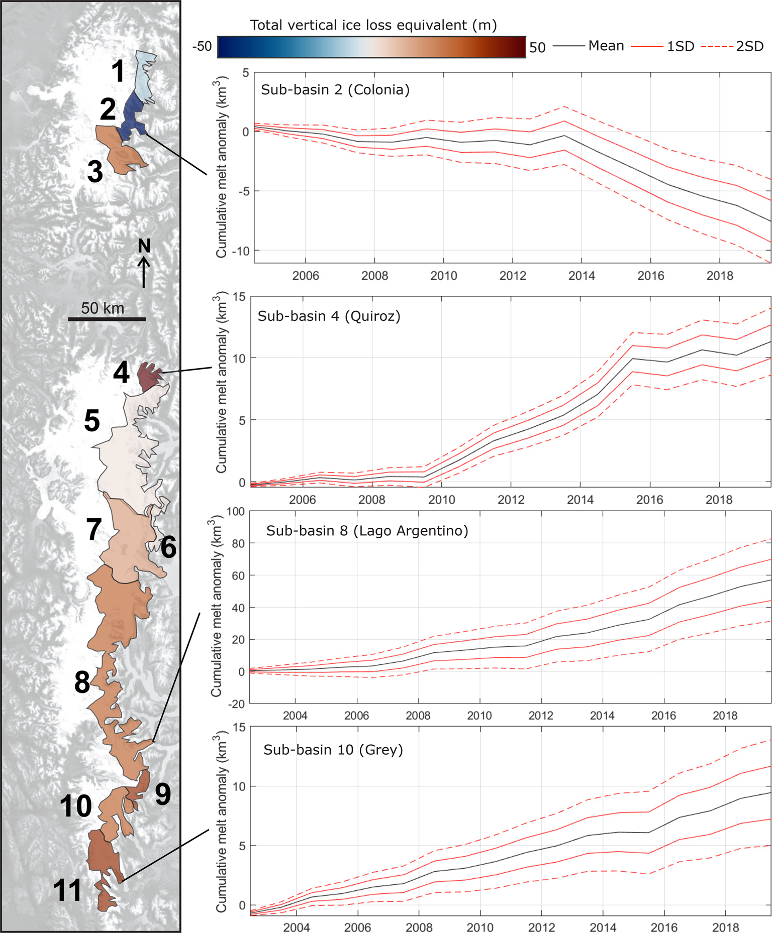
Fig. 5. Time-integrated rGVL anomaly δ[ − dI/dt]C of the different Patagonian Icefield sub-basins, in km3. Sub-basin color is scaled according to the total excess volume loss, in meters of vertical ice loss over the 2006–2019 study period. Uncertainties are generally higher in sub-basins with higher non-glaciated areas (e.g. sub-basin 2; sub-basin 8), and lowest in sub-basins that are almost entirely glaciated (e.g. sub-basin 4).
We sum the rGVL anomaly across the entire sector of the Patagonian Icefields drained by these rivers (Fig. 6). This shows a total negative ice volume anomaly of 135 ± 50 km3 over 2006–2019, relative to the 2000–2005 reference period, which would raise global sea levels by 0.37 ± 0.14 mm, or 0.027 ± 0.01 mm of sea level rise per year. Total vertical ice loss equivalent varies from −51 m (relative decrease in thinning) in sub-basin 2 to +113 m in sub-basin 4 (Fig. 2). Six out of the 11 basins have vertical ice loss equivalents exceeding 25 m, including all of the southernmost basins (8, 9, 10 and 11).
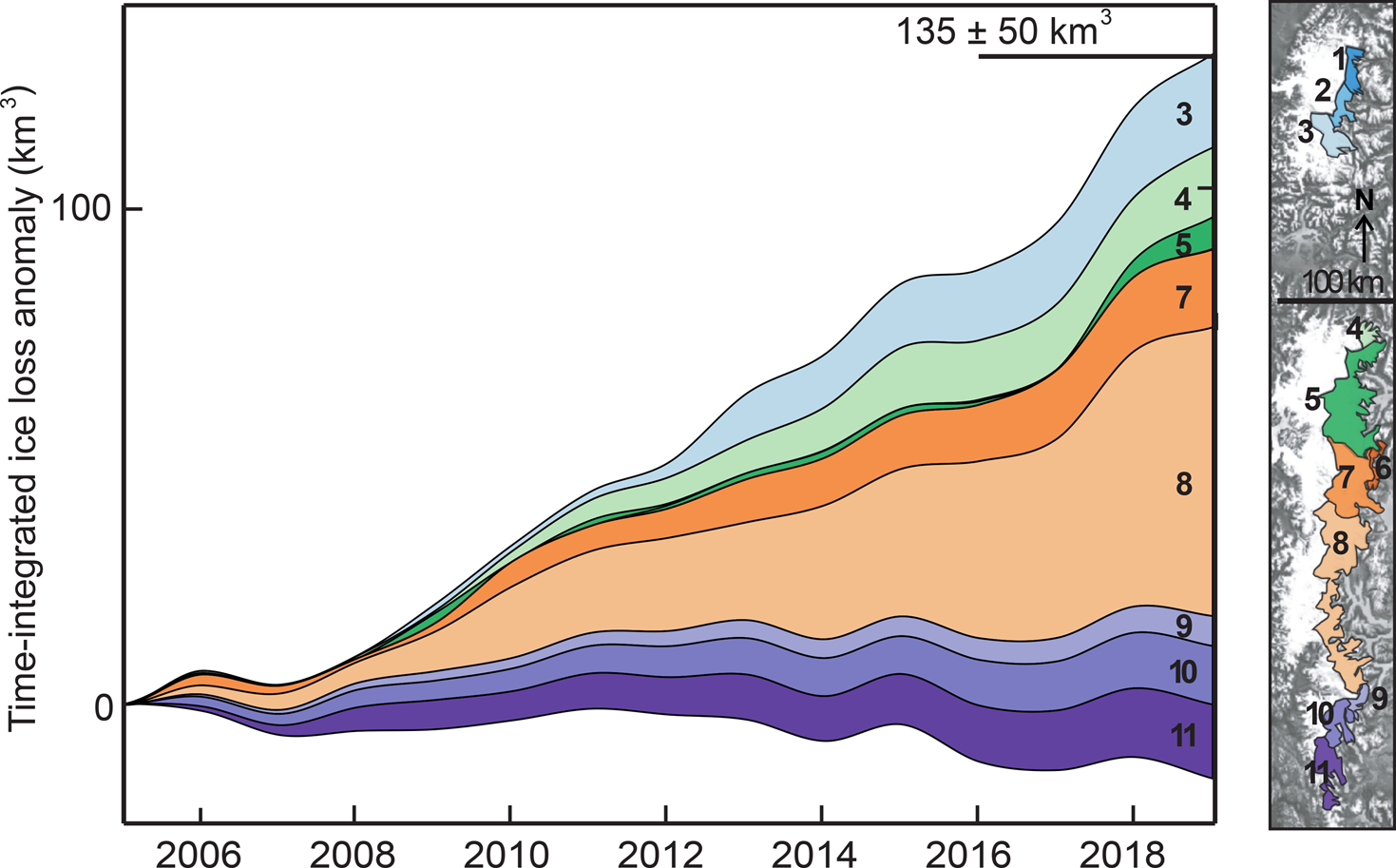
Fig. 6. Stacked volume loss for all sub-basins in the NPI and SPI. The time-integrated rGVL anomaly over the study period (2006–2019) is 135 ± 50 km3 - relative to a total SPI and NPI volume of 4, 756 ± 923 km3. Note that basins 8 (Lago Argentino) has the largest individual rGVL anomaly. Note also that the lower bound of the envelope overlaps into negative values due to a negative rGVL anomaly in some areas, particularly in sub-basin 2.
3.3. Average anomaly and anomaly slope
The time-averaged rGVL anomaly evaluates whether the rate of glacier volume loss has increased or decreased through time. Nine out of 11 sub-basins exhibit a positive time-averaged rGVL anomaly (sub-basins 3–11), while two exhibit a negative time-averaged rGVL anomaly (sub-basins 1 and 2). Sub-basin 4 (Glaciar Quiroz) exhibits the largest time-averaged rGVL anomaly at 7.06 ± 1.69 m a−1 (units of vertical ice loss equivalent), followed by 8 (Lago Argentino) and sub-basins 9 (Lago Dickson) at 2.01 ± 0.91 m a−1 and 1.98 ± 1.08 m a−1 respectively (Fig. 7b). Sub-basin 2 has a negative time-averaged rGVL anomaly of −3.18 ± 1.48 m a−1. Three sub-basins, 1, 5, and 6, have time-averaged rGVL anomaly ranges overlapping with zero (−0.51 ± 1.97 m a−1, 0.15 ± 0.57 m a−1 and −0.01 ± 0.60 m a−1 respectively).
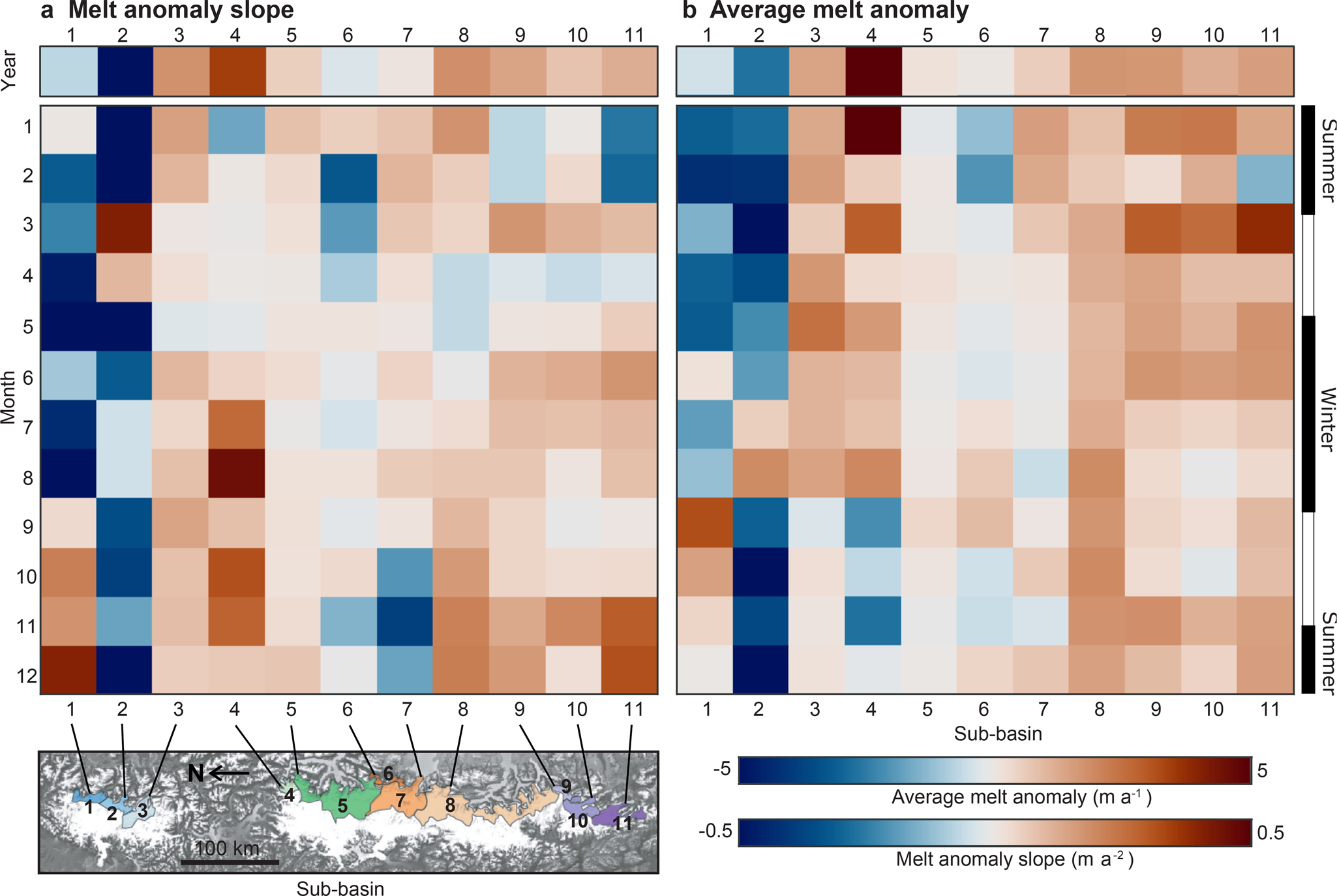
Fig. 7. rGVL anomaly slope (a) and time-averaged rGVL anomaly (b) for the annual and monthly time series.
The slope of the annual rGVL anomaly time series record any acceleration or deceleration in the rate of ice volume change over our 2006–2019 study period. Eight out of 11 sub-basins (3–5 and 7–11) have accelerating volume loss, and three sub-basins (1,2, and 6) have decelerating volume loss. However, the 2 standard-deviation uncertainty envelope of rGVL anomaly slopes overlaps with 0 in all but three cases: sub-basin 2 (−0.53 ± 0.35 m a−2), sub-basin 8 (0.18 ± 0.09 m a−2), and sub-basin 9 (0.14 ± 0.09 m a−2).
Monthly volume-loss anomalies (the same month, across different years) provide information about the seasonality of the rate of glacier volume loss. We evaluate a total of 132 trends in the rate of glacier volume loss – 12 different months for each of the 11 sub-basins (Fig. 7). Just under two-thirds (88) of the time-averaged monthly glacier-volume-loss anomalies are positive, with 17% (23) greater than 1 m of ice loss per year. Conversely, 6% (8) have negative time-averaged monthly glacier-volume-loss anomalies equivalent to more than 1 m of ice gain per year. Less than 10% (11) of time-averaged monthly rGVL anomalies have two standard deviation ranges overlapping with zero. The changes in the rate of ice volume loss are unevenly distributed through the different months of the year. Five sub-basins have their greatest time-averaged monthly glacier-volume-loss anomalies at the start of the melt season (August-September; sub-basins 1, 2, 5, 6, and 8), two have it in mid-summer (January; sub-basins 4 and 7), and three have it at the end of the melt season (March; sub-basins 9, 10, and 11). Sub-basin 3 is an exception, having its greatest increase in the rate of volume loss in the mid-winter (May).
3.4. Mann-Kendall results
The Mann-Kendall p-value of the time-integrated rGVL anomaly tests the null hypothesis that the rate of glacier volume loss is neither increasing nor decreasing over the study period. This is equivalent to testing whether the mean of the annual rGVL anomaly differs from zero. Eight out of 11 sub-basins (2, 3, 4, 7, 8, 9, 10, and 11) exhibit monotonic trends in their time-integrated glacier-volume-loss anomalies (Fig. 8b). The trends in each of these sub-basins are all highly statistically significant (p < 0.001). The Mann-Kendall test itself does not provide the sign of each significantly monotonic trend, which we obtain from the time-averaged rGVL anomaly.
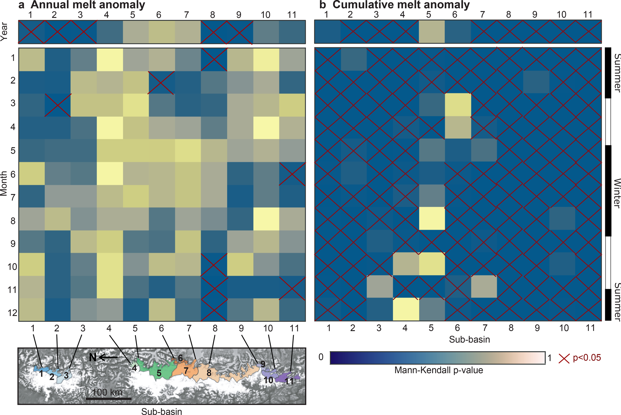
Fig. 8. Mann-Kendall test p-values for both the annual rGVL anomaly (a) and time-integrated rGVL anomaly time series (b). Most of time series exhibit significant trends in time-integrated rGVL anomaly, but that significant trends in the annual rGVL anomaly are rarer. Significant trends are highlighted by red crosses.
The annual rGVL anomaly Mann-Kendall p-value tests the null hypothesis that the change in rate of glacier volume loss is constant through time (no acceleration or deceleration). Five out of 11 sub-basins (1, 2, 3, 8, and 9) exhibit monotonic trends in their annual volume-loss anomalies (Fig. 8a) significant at the 95% level (p < 0.05), although only two of these trends are significant at the 99.9% level (sub-basins 2 and 8; p < 0.001).
We reproduce the same Mann-Kendall test for each of the 12 individual monthly (single month across multiple years) time series for each of the 11 sub-basins. Three sub-basins (1, 8, and 11) have a Mann-Kendall p <0.05 for all 12 of their monthly time-integrated rGVL anomaly. 80% of monthly time-integrated rGVL anomaly time series (108) exhibit monotonic trends significant at the 95% level. Very few months exhibit significant trends in monthly volume-loss anomalies, with only 4 out of 11 sub-basins having a single monthly p-value less than 0.05. Only one out of the 132 monthly time series exhibits a monthly rGVL anomaly significant at the 99.9% level (November in sub-basin 8).
4. Discussion
4.1. Multiannual and seasonal glacier volume change
Spatially averaged across all basins, the rate of glacier-volume loss is increasing by 9.6 ± 3.6 km3 a−1. Integrated over our 2006–2019 study period, this represents 135 ± 50 km3 of additional volume loss over 2000–2005 levels. Joint interpretation of this anomaly with a Mann-Kendall test shows that 7 out of 11 sub-basins exhibit positive ice-loss trends significant at the 99.9% level, including all sub-basins in the central and southern section of the SPI. One sub-basin, Glaciar Colonia (sub-basin 2), shows a highly significant (99.9% level) decrease in the rate of ice loss, suggesting that it may be past peak water.
Several sub-basins also exhibit significant positive rGVL anomaly slopes, representing accelerating volume loss. This is particularly pronounced in sub-basin 8 (Lago Argentino) which exhibits an 2.01 ± 0.91 m a−1 increase in glacier melt rate and a 0.18 ± 0.09 m a−2 increase in the slope of glacier melt rate (acceleration), both being significant to the 99.9% level. Similarly, Glaciar Colonia (sub-basin 2) exhibits a 0.53 ± 0.35 m a−2 decrease in the slope of glacier melt rate (deceleration) significant at the 99.9% level. This significant increase in the rate of glacier volume loss in several sub-basins highlights possible non-linear interactions between warming temperatures and glacier volume loss, including elevation-related feedbacks (Bolibar and others, Reference Bolibar, Rabatel, Gouttevin, Zekollari and Galiez2022) and lacustrine calving processes (Skvarca and others, Reference Skvarca, Raup and Angelis2003; Saito and others, Reference Sakakibara, Sugiyama, Sawagaki, Marinsek and Skvarca2013; Sugiyama and others, Reference Sugiyama2016).
Seasonal changes in the rate of glacier-volume loss are consistent with a lengthening of the melt season: 5 sub-basins exhibit their greatest time-averaged monthly glacier-volume-loss anomalies at the beginning of the melt season in late winter to early spring (August–September), and a further three sub-basins exhibit their greatest time-averaged monthly glacier-volume-loss anomalies at the end of the melt season (March). With the exception of sub-basins 1 and 2, almost all months have a positive rGVL anomaly, suggesting that glaciers are losing additional volume throughout the year.
Throughout the remainder of this section, we discuss some limitations of this method, the importance of these results relative to other datasets, and their relevance to assessments of sea-level rise and future volume loss of the Patagonian Icefields.
4.2. Limitations and uncertainties
Assessments of ice melt using proglacial river discharge data are subject to two main limitations:
-
Spatial resolution: River discharge is inherently an integrative measurement, providing a measure of the total rate of ice volume loss across the entire drainage basin above the gauging station. Unless used in conjunction with other (e.g. satellite based) monitoring techniques, it cannot determine the spatial pattern of ice loss at a finer resolution than the scale of the drainage basin. Rapid ice loss at one glacier could therefore be masked by modest ice gain over a different, larger glacier or vice-versa.
-
Multiple sources of uncertainties: As we have demonstrated in our methods section, calculating the rate of glacier volume loss anomaly from a discharge anomaly requires a correction for other inputs into the hydrological system. The techniques required to monitor these different contributions and the associated uncertainties may vary through time in a rapidly evolving proglacial environment (Carrivick and Heckmann, Reference Carrivick and Heckmann2017; Carrivick and Tweed, Reference Carrivick and Tweed2021). The uncertainty associated with final estimates of ice volume loss incorporate the uncertainties from both the discharge record itself and each of the corrections (e.g. rainfall, evapotranspiration, etc.). Glaciers with a low rate of volume change, or ice loss signals in basins with only a small fraction of glacier cover will have a low signal to noise ratio, and in extreme cases the ice loss signal could be masked entirely.
We made a simplifying assumption that the change in lakewater storage was the dominant change in overall terrestrial water storage, excluding any change in groundwater, permafrost, wetland, rock glacier or other possible terrestrial water storage terms. No high-resolution regional data on each of these terms is currently available for Patagonia, which precludes their inclusion in our water balance calculation. Several recent studies have improved our understanding of different aspects of this problem (e.g. Alvarez-Garreton and others, Reference Alvarez-Garreton2018; Zalazar and others, Reference Zalazar2020), and if suitable data is available in the future this should be included in new versions of this workflow.
For the first limitation (spatial resolution), we consider that this method is complementary to existing field and remote-sensing based methods. Proglacial discharge-based methods can calculate a basin-wide estimate of total glacier volume change at high temporal resolution, while remote sensing techniques will commonly provide the spatial pattern of ice thinning for a single time period. For the second limitation, it is important to account for and propagate the uncertainties of each of the contributing datasets. In our case, both the rate of glacier volume loss and the ice cover fraction in each drainage basin are high, resulting in high signal-to-noise ratios and a resolvable ice loss signal in most cases (e.g. Fig. 5).
4.3. Controls on ice loss and future glacier evolution
Our results show a heterogeneous pattern of ice loss both in time and in space. The ice volume loss anomaly will depend on several factors, including (i) the baseline rate of ice volume loss during the reference period, (ii) the total volume of ice available to melt in a given sub-basin, (iii) the frontal conditions and rate of frontal ablation of glaciers, (iv) changes in glacier surface mass balance, including increased surface ablation. Temperature in our study area has increased by an average of $0.59\pm 0.07\, ^\circ$ C by 2015–2019 relative to reference period of 1940–1980, and $0.54\pm 0.04\, ^\circ$
 C relative to a reference period of 2000–2005 (supplementary section S2). The degree of warming is slightly higher for the most southerly basins ($0.63\pm 0.02\, ^\circ$
 C relative to $0.56\pm 0.04\, ^\circ$
 C for the three most northerly basins, all relative to a 1940–1980 reference period). The temperature record shows that warming has been on the order of half a degree for all sub-basins, and that the majority of this warming has occurred within our 21st century study period. Our regional pattern of increasing rates of ice loss is likely forced by this warming, but the warming does not explain the complex spatial and temporal pattern of ice volume loss anomaly which we observe.
Our 11 sub-basins contain a total of 2423 km3 of ice (Carrivick and others, Reference Carrivick, Davies, James, Quincey and Glasser2016; Millan and others, Reference Millan2019), or just under half of the volume of the Patagonian Icefields according to a volume estimate from close to the end of our study period (supplementary section S3). The majority of this ice is present in sub-basins 5 (O'Higgins/San Martín; 753 km3), sub-basin 8 (Lago Argentino; 565 km3), and sub-basin 7 (Lago Viedma; 564 km3). Sub-basins 4 (Quiroz), 6 (El Chaltén), and 9 (Dickson) have ice volumes of less than 25 km3. The time-integrated volume loss anomaly is, however, not proportional to the total volume in each basin: this anomaly is as high as 83 ± 20% of the remaining volume in small sub-basin 4 (Quiroz), 24 ± 13% in sub-basin 9 (Dickson), and 13 ± 8% in sub-basin 3 (Colonia). Sub-basin 6 (Lago Argentino) has the largest time-integrated volume loss anomaly, which represents 12 ± 5% of its total ice volume. The time-integrated volume loss anomaly represents a negligible proportion (0%) of the total ice volume in sub-basins 5–7 (O'Higgins/San Martín, El Chaltén, and Lago Viedma). The sub-basins in which the volume loss anomaly represents the greatest proportion of present-day ice volume have all experienced rapid ice-contact lake growth within our study period. In sub-basins 3 (Colonia), 4 (Quiroz), and 9 (Dickson), glacier retreat has opened up new ice-contact lakes at previously land-terminating glaciers. In sub-basin 8 (Lago Argentino) both the main lake and several marginal ice-contact lakes (Lago Guillermo at Glaciar Upsala, and lakes at Glacier Onelli, Mayo, and Ameghino). In contrast, the very large lake-terminating glaciers in sub-basin 5 (Lago O'Higgins/San Martín) and sub-basin 7 (Lago Viedma) have experienced only minor area changes over the study period. Sub-basin 2 (Nef) experienced rapid frontal retreat and lake growth during the 2000–2005 reference period, and stabilized during the study period. Overall, we see that the order volume loss anomaly pattern between different sub-basins correlates with the growth and evolution of ice-contact lakes. While warming temperatures drive the overall increase in rates of ice volume loss, the spatial and temporal distribution of this volume loss is modulated by changes in ice-contact lakes.
None of our study areas contain large land-terminating glaciers by the end of our study period and this ice volume loss method cannot be applied to tidewater glaciers, so we do not assess the relative changes of land, lake, and marine terminating glaciers. Both numerical models (e.g., Sutherland and others, Reference Sutherland2020; Carrivick and others, Reference Carrivick2022) and remote observations (e.g., Baurley and others, Reference Baurley, Robson and Hart2020; Mallalieu and others, Reference Mallalieu, Carrivick, Quincey and Raby2021; Carrivick and others, Reference Carrivick2022) ranging from New Zealand to Greenland have shown that ice-contact lakes may both initiate and accelerate glacier retreat. Our results are consistent with this and further emphasize that ice-contact lakes must be accounted for when forecasting future ice volumes.
We consider our rGVL anomalies from the perspective of peak water and in the context of glacier shrinkage. Any sub-basin with a positive time-averaged rGVL anomaly has likely not reached peak water, while any sub-basin with a negative time-averaged rGVL anomaly has likely passed peak water. Sub-basins 3 (Colonia), 4 (Quiroz), 7 (Lago Viedma), 8 (Lago Argentino), 9 (Lago Dickson), 10 (Grey), and 11 (Tyndall) all have a statically significant positive time-averaged glacier-volume-loss anomalies, consistent with increasing rates of volume loss and a pre-peak water drainage basin. Sub-basin 2 (Nef) exhibits a negative time-averaged rGVL anomaly. Glaciar Nef has a ~180 km2 upstream catchment area constrained by steep terrain on the East flank of the NPI, and an accumulation area ratio of only 0.6 (Minowa and others, Reference Minowa, Schaefer, Sugiyama, Sakakibara and Skvarca2021). Altogether, this suggests that the Glaciar Nef basin may have already passed peak-water and be on the decreasing limb of the volume loss trend. Sub-basin 1 (Glaciar Leones and Soler) also exhibits a neutral or weak negative time-averaged rGVL anomaly and may be close to peak-water at present day.
Our findings are broadly consistent with the model outputs of Huss and Hock (Reference Huss and Hock2018), who evaluated the likely timing of peak water for the Rio Baker (sub-basins 1, 2, and 3) and Rio Santa Cruz (sub-basins 6, 7, and 8). Their modeled peak water for the Rio Baker ranged from 2015 ± 18 for RCP2.6 to 2020 ± 16 for RCP8.5, consistent with our finding that some sub-basins are at (sub-basin 1) or past (sub-basin 3) peak water in this drainage basin. For the Rio Santa Cruz, they calculate a peak water timing ranging from 2050 ± 18 for RCP2.6 to 2096 ± 9 for RCP8.5. The two large sub-basins in this drainage basin (sub-basins 7 and 8) both have increasing rates of rGVL, consistent with this pre-peak-water status. Their model predicts that the annual glacier runoff would increase between 14 and 48% between 1980–2000 and peak water for the Rio Santa Cruz basin (Huss and Hock, Reference Huss and Hock2018). Depending on the external forcings applied, glaciers may either transition to a new steady state or disappear entirely following the decreasing volume loss period of decreasing rates of glacier loss. While the projected future decrease in glacier runoff is of less relevance for water resources in Patagonia relative to the Tropical Andes or Himalaya, it may affect the supply of water to newly constructed hydroelectric projects and reduce power generation (Tagliaferro and others, Reference Tagliaferro, Miserendino, Liberoff, Quiroga and Pascual2013) and exacerbate regional droughts (Garreaud, Reference Garreaud2018).
We calculate a sea-level-equivalent total rGVL anomaly of 0.37 ± 0.14 mm for our study period of 2006–2019, or 0.027 ± 0.01 mm a−1. This third of a mm of sea level rise represents only the additional ice-volume loss over 2000–2005 levels of the glacierised basins draining the rivers analyzed in this study, not the total contribution of the Patagonian Icefields to sea-level rise, which Abdel Jaber and others (Reference Abdel Jaber, Rott, Floricioiu, Wuite and Miranda2019) estimated at 0.048 ± 0.002 mm a−1 for the period 2000–2012 (total of 0.624 ± 0.026 mm).
4.4. Comparison to remotely sensed datasets
Direct comparison of our findings to remotely sensed data is limited by the spatial and temporal resolution of each dataset. We subdivide remote-sensing-based studies into three categories: (1) Indirect measurements of glacier mass loss, for example, through gravity-field changes (Chen and others, Reference Chen, Wilson, Tapley, Blankenship and Ivins2007; Jacob and others, Reference Jacob, Wahr, Pfeffer and Swenson2012; Lange and others, Reference Lange2014; Richter and others, Reference Richter2016, Reference Richter2019). (2) Image-based measurements of glacier frontal ablation or areal change (Davies and Glasser, Reference Davies and Glasser2012; Sakakibara and Sugiyama, Reference Sakakibara and Sugiyama2014; Hata and Sugiyama, Reference Hata and Sugiyama2021; Minowa and others, Reference Minowa, Schaefer, Sugiyama, Sakakibara and Skvarca2021). (3) Direct measurements of changes in ice-surface elevation or ice volume, through satellite altimetry (Foresta and others, Reference Foresta2018) or differencing of repeat digital elevation models (Rignot and others, Reference Rignot, Rivera and Casassa2003; Willis and others, Reference Willis, Melkonian, Pritchard and Rivera2012; Malz and others, Reference Malz2018; Dussaillant and others, Reference Dussaillant2019; Abdel Jaber and others, Reference Abdel Jaber, Rott, Floricioiu, Wuite and Miranda2019; Minowa and others, Reference Minowa, Schaefer, Sugiyama, Sakakibara and Skvarca2021; Hugonnet and others, Reference Hugonnet2021).
4.4.1. Indirect measurements
The Gravity Recovery and Climate Experiment (GRACE) was a twin-satellite mission that measured anomalies in the Earth's gravitational field between 2002 and 2017. As glaciers lose mass, they locally reduce gravitational potential. Multiple studies have used this to investigate mass loss rates of the Patagonian Icefields, finding comparable mass loss rates of −27.9 ± 11 km3 a−1, (Chen and others, Reference Chen, Wilson, Tapley, Blankenship and Ivins2007), −23 ± 9 Gt a−1 Jacob and others (Reference Jacob, Wahr, Pfeffer and Swenson2012), −24.4 ± 4.7 Gt a−1 (Richter and others, Reference Richter2019), and −23.5 ± 8.1 Gt a−1 (Li and others, Reference Li, Chen, Ni, Tang and Hu2019, Table 2). Richter and others (Reference Richter2019)'s study of Patagonian mass loss over the entire GRACE operating period shows rapid ice loss, but no evidence for an increase in ice loss over the 21st century (even with corrections for changes in terrestrial water storage, GIA, and other factors; see Appendix A of Richter and others (Reference Richter2019)). Li and others (Reference Li, Chen, Ni, Tang and Hu2019) show a more complex temporal pattern, with an apparent slowdown in mass loss over the period 2008–2012 and high mass loss in 2002–2007 and 2013–2016 (Table 2).
Table 2. Rate of volume loss of the Patagonian Icefields measured from a range of different techniques.
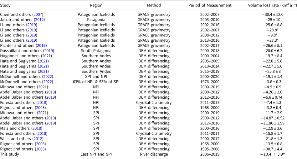
Where results were measured or reported in units of mass loss (i.e. those studies using GRACE gravimetry and CryoSat-2 altimetry), we converted to ice volume using a density of 917 kg m−3. Note that the precise study region varies between the different studies.
*No uncertainty given for these values.
${\dagger}$ Values in the present study are an anomaly over 2000–2005 levels instead of an absolute ice loss value.
Overall, gravity-based observations of the Patagonian Icefields suggest a much steadier ice loss than observed in this study. Resolving a different signal from the NPI and SPI is at the limit of GRACE's resolution (Richter and others, Reference Richter2019). This resolution was estimated at around 63 000 km2 or 250 by 250 km for an error level of ≤2 cm (Vishwakarma and others, Reference Vishwakarma, Devaraju and Sneeuw2018). The scale of the sub-basins used in this study (Fig. 2) is therefore smaller than GRACE's spatial resolution and the increased rates of glacier volume loss we observe from hydrograph separation could be masked by reduced rates of glacier volume loss or even volume gain (Rivera and Casassa, Reference Rivera and Casassa1999; Hata and Sugiyama, Reference Hata and Sugiyama2021) on the summit of the icefields or West-draining tidewater glaciers. We see no evidence of the 2008–2012 slowdown in the rate of mass loss which Li and others (Reference Li, Chen, Ni, Tang and Hu2019) propose.
4.4.2. Frontal ablation
Glacier volume loss can occur through melting of the ice surface (negative surface volume balance), retreat of the ice front (calving and other frontal retreat), and draw-down of ice as a result of increased flow velocity (dynamic thinning). Glacier frontal ablation is defined as the sum of two terms: (1) changes in the position of the ice front, and (2) the flux of ice across the front. A fast-flowing glacier can, therefore, have a high frontal ablation rate (Sakakibara and Sugiyama, Reference Sakakibara and Sugiyama2014; Minowa and others, Reference Minowa, Schaefer, Sugiyama, Sakakibara and Skvarca2021) despite losing no volume. In addition, glacier speed-up can increase frontal ablation and the rate of volume loss even in the absence of frontal retreat – with the volume loss being compensated by dynamic thinning of the glacier up-ice from the front. Minowa and others (Reference Minowa, Schaefer, Sugiyama, Sakakibara and Skvarca2021) reveal periods of rapid acceleration of frontal ablation related to glacier speed-ups, such as the 2008-2011 acceleration and retreat at Upsala (Saito and others, Reference Sakakibara, Sugiyama, Sawagaki, Marinsek and Skvarca2013; Minowa and others, Reference Minowa, Schaefer, Sugiyama, Sakakibara and Skvarca2021). A high-flow and high-δ[ − dI/dt] year occurred in sub-basin 8 (which contains Glaciar Upsala) in 2008, at the same time as the high frontal ablation observed by Minowa and others (Reference Minowa, Schaefer, Sugiyama, Sakakibara and Skvarca2021). However, given that frontal ablation only accounts for one component of the total glacier mass-balance, we cannot directly compare it to our glacier-volume-loss anomalies.
4.4.3. Surface elevation change
Surface elevation measurements of the NPI and SPI have been acquired using swath radar altimetry (Foresta and others, Reference Foresta2018) and a range of DEMs constructed from both optical and radar imagery (e.g. Abdel Jaber and others, Reference Abdel Jaber, Rott, Floricioiu, Wuite and Miranda2019; Hugonnet and others, Reference Hugonnet2021). All measurement techniques are subject to limitations, in particular the frequent cloud cover for optical measurements and unknown surface-penetration depths for radar-based methods. Volume-loss calculations from a range of studies show agreement that the Patagonian Icefields have been losing more than 10 km3 a−1 of ice over the 21st century, although there are large deviations between individual measurements (Table 2).
Direct comparisons to the results of this study are challenging, as all of the prior studies have a multiannual temporal resolution, many cover slightly different study regions (Table 2), and none investigate the seasonal pattern of ice loss. Only Abdel Jaber and others (Reference Abdel Jaber, Rott, Floricioiu, Wuite and Miranda2019), Hugonnet and others (Reference Hugonnet2021), and McDonnell and others (Reference McDonnell, Rupper and Forster2022) present results from more than a single time period. Abdel Jaber and others (Reference Abdel Jaber, Rott, Floricioiu, Wuite and Miranda2019)'s data includes two time periods (2000–2012 and 2012–2016) and suggests that the rate of ice volume loss increased in the NPI and decreased in the SPI over time (Table 2). Hugonnet and others (Reference Hugonnet2021) present binned 5-yearly measurements of ice loss across the Southern Andes, which show an increase in the rate of volume loss for each subsequent period (albeit all having large uncertainties). The 2015–2019 time-period shows a 6.1 km3 a−1 rGVL anomaly above 2000–2004 levels – comparable to the 9.63 ± 1.80 km3 a−1anomaly observed in this study over the eastern portion of the NPI and SPI (Table 2 and Fig. 6). McDonnell and others (Reference McDonnell, Rupper and Forster2022) highlight how sub-sampling of elevation loss maps can lead to biases in regional mass balance estimates. They show that when comparing the same glaciers between 1979–2000 and 2000–2020, ice loss on the NPI has increased by a factor of 1.2 and ice loss on the SPI has increased by a factor of 2.4.
The limited agreement between different studies and high uncertainties of individual measurements make the assessment of the rate of volume loss from remotely sensed elevation data challenging. All studies, however, indicate rapid rates of volume loss in the land- or lake-terminating eastern margins of the SPI and NPI considered in this study, which exhibit some of the most rapid ablation rates (locally exceeding 10 m a−1) of any region on Earth (Dussaillant and others, Reference Dussaillant2019; Zemp and others, Reference Zemp2019). In addition, the two most recent studies considering multiple time period of elevation changes (Hugonnet and others, Reference Hugonnet2021; McDonnell and others, Reference McDonnell, Rupper and Forster2022) show an increase in the rate of ice loss over time for both the SPI and NPI, consistent with our findings.
5. Conclusions
We used the hydrological balance of Patagonian glacierised river basins to calculate changes in the rate of NPI and SPI glacier volume loss. We combine proglacial discharge data with remotely sensed climate data to isolate the contribution of glacier volume loss to river discharge. We divide the Patagonian Icefields into 11 sub-basins in which streamflow data is publicly available and calculate the rate of volume loss in each relative to a reference period of 2000-2005. Seven sub-basins exhibit statistically significant increases in rate of volume loss, with a whole-study-period (2006–2019) integrated volume loss anomaly of 135 ± 50 km3 across all 11 sub-basins. The rGVL anomaly is spatially heterogeneous, with the anomaly as high as 7.06 ± 1.69 m a−1 in one sub-basin (Glaciar Quiroz) and two out of three sub-basins in the NPI exhibiting a negative rGVL anomaly over the period of study. The greatest increase in glacier volume loss occurred early and late in the melt season, although volume loss increased throughout most or all months of the year in most sub-basins. The total rGVL anomaly is equivalent to 0.027 ± 0.01 mm a−1 of sea level rise atop background contributions from the Patagonian Icefields and highlights the rapid and accelerating rates of volume loss at Patagonia's lake-terminating glaciers.
Supplementary material
The supplementary material for this article can be found at https://doi.org/10.1017/jog.2023.9.
Data
All the data used in this study is publicly available from the respective sources. All river discharge data and lake level data for Chile is available from the SNIA (https://snia.mop.gob.cl158/BNAConsultas/reportes) and that for Argentina is available from BDHI (http://bdhi.hidricosargentina.gob.ar). GPM-IMERG precipitation and MOD16A2 evapotranspiration data are available from various online sources, and in our case were downloaded using Google Earth Engine.
Acknowledgements
MV was supported by a University of Minnesota College of Science and Engineering Fellowship and a Doctoral Dissertation Fellowship. This material is based upon work supported by the National Science Foundation under Grant No. EAR-1714614, coordinated by Lead PI Maria Beatrice Magnani. Ng received support from NSF Award EAR-1759071. This manuscript was greatly improved by suggestions from two anonymous reviewers.


 Open access