


1. Introduction
Plane Couette (PC) flow, the fluid motion between two parallel flat plates moving at different speeds, is one of the simplest canonical configurations for the numerical study of wall turbulence – its statistics and dynamics. In contrast to the extensive study of plane Poiseuille (PP) flows (e.g. Kim, Moin & Moser Reference Kim, Moin and Moser1987; Lee & Moser Reference Lee and Moser2015; Hoyas et al. Reference Hoyas, Oberlack, Alcántara-Ávila, Kraheberger and Laux2022), much less attention has been paid to the PC flow. One of the main reasons is that PC flow contains large-scale structures (streamwise-oriented rollers), distributed in counter-rotating pairs across the spanwise domain whose resolution requires an extended computational domain in both the streamwise and spanwise directions. The first direct numerical simulation (DNS) of turbulent PC flows was conducted by Lee & Kim (Reference Lee and Kim1991) at the friction Reynolds number  $Re_\tau =170$ with lengths
  $4{\rm \pi} h\times 8 {\rm \pi}/3 h$ in the streamwise and spanwise directions. Here,
  $h$ denotes half-channel-height. They found that the most energetic motion at the channel centre occurs at wavenumber
  $k_x h=0$ and
  $k_zh=1.5$. Later, Komminaho, Lundbladh & Johansson (Reference Komminaho, Lundbladh and Johansson1996) and Tsukahara, Kawamura & Shingai (Reference Tsukahara, Kawamura and Shingai2006), respectively, performed DNS at
  $Re_\tau =52$ and
  $Re_\tau =126$ with a relatively large domain (i.e.
  $28{\rm \pi} h \times 8{\rm \pi} h$ for the former and
  $64 h \times 6 h$ for the latter). Avsarkisov et al. (Reference Avsarkisov, Hoyas, Oberlack and Garcia-Galache2014) conducted DNS at
  $Re_\tau$ up to
  $550$ and showed that the mean velocity profile exhibits a logarithmic region with a slope of
  $0.41$. DNSs for
  $Re_\tau$ up to
  $986$ by Pirozzoli, Bernardini & Orlandi (Reference Pirozzoli, Bernardini and Orlandi2014) showed a secondary outer peak in the streamwise turbulent intensity at the highest
  $Re_\tau$ – related to the presence of the large-scale rollers of spanwise wavelength
  $\lambda _z\approx 5h$. Despite these prior studies, the characteristics of these large-scale motions remain elusive. Lee & Moser (Reference Lee and Moser2018) performed DNS with a very large computational domain (viz.
  $100{\rm \pi} h \times 5{\rm \pi} h$) for
  $Re_\tau$ up to
  $500$. They found that as
  $Re_\tau$ increases, the large-scale structures become more coherent in the streamwise direction. Recently, Cheng, Pullin & Samtaney (Reference Cheng, Pullin and Samtaney2022) performed wall-resolved as well as wall-modelled large-eddy simulation (LES) of PC flows at
  $Re_\tau$ up to
  $2600$ and
  $2.8\times 10^5$, respectively. Interestingly, the energy of the large-scale streamwise rollers was found to decrease with increasing
  $Re_\tau$.
Even fewer studies have targeted the compressible PC flow – most focusing on the linear stability analysis (Chagelishvili, Rogava & Segal Reference Chagelishvili, Rogava and Segal1994; Duck, Erlebacher & Hussaini Reference Duck, Erlebacher and Hussaini1994; Hu & Zhong Reference Hu and Zhong1998; Ramachandran et al. Reference Ramachandran, Saikia, Sinha and Govindarajan2016). For example, Duck et al. (Reference Duck, Erlebacher and Hussaini1994) showed that, unlike the incompressible equivalent, linear unstable modes exist in compressible PC flow. Malik, Dey & Alam (Reference Malik, Dey and Alam2008) investigated the linear stability and the non-modal transient growth for both the uniform shear flow with constant viscosity and the non-uniform shear flow with stratified viscosity. They found that both mean flows are linearly unstable for a range of supersonic Mach numbers. Using the resolvent analysis, Dawson & McKeon (Reference Dawson and McKeon2019) studied how the shape and amplitude of the optimal disturbances depend on the Mach number in compressible laminar PC flow.
Regarding DNS of compressible PC flow, the first study was performed by Buell (Reference Buell1991) at bulk Reynolds number  $Re_b=3000$ and bulk Mach number
  $M_b$ up to
  $3$. He found that the large-scale streamwise rollers become less organized at higher
  $M_b$. Szemberg O'Connor's (Reference Szemberg O'Connor2018) DNS of compressible PC at two different bulk-to-shear viscosity ratios showed that the bulk (dilatational or second) viscosity has a minor effect on mean flow quantities. To derive an eddy conductivity closure for wall-modelled LES of high-speed flows, Chen et al. (Reference Chen, Lv, Xu, Shi and Yang2022) recently performed DNS of compressible PC flow with different wall temperatures for wall Mach numbers
  $M_w$ up to 6.
The present work aims to systematically examine the compressibility effect on PC flow, mainly focusing on how Reynolds and Mach numbers affect turbulence statistics and structures. The remaining paper is organized as follows. Section 2 presents the simulation methods and parameters. Section 3 discusses the main results, including turbulence statistics and structures. Conclusions are drawn in § 4.
2. Numerical set-up
2.1. Numerical method
The DNS of the compressible Navier–Stokes equation for the PC flow (figure 1) is conducted with our in-house code (Yao & Hussain Reference Yao and Hussain2020). The fluid considered is a perfect gas governed by Sutherland's viscosity law. The seventh-order upwind-biased and eighth-order centred schemes are used for the convective and viscous terms, respectively (Li et al. Reference Li, Fu, Ma and Liang2010). The low-storage third-order Runge–Kutta algorithm is utilized for time integration. See Yao & Hussain (Reference Yao and Hussain2020) for more details on the governing equations and the simulation methods. The DNS is conducted in a truncated rectangular box with the dimensions  $L_x$,
  $L_y$,
  $L_z$ in the streamwise (
 $x$), wall-normal (
 $y$) and spanwise (
 $z$) directions. Periodic boundary conditions are specified in the wall-parallel (
 $x,z$) directions with constant mesh size, and a mapping function is used in the wall-normal direction. The top and bottom walls move in the streamwise direction with equal and opposite speeds
  $\pm U_w$, and the isothermal boundary condition is employed for the temperature at the walls
  $T_w$. The solver has been extensively validated in our previous works (Yao & Hussain Reference Yao and Hussain2019, Reference Yao and Hussain2020) for PP configuration. In Appendix A, the code is further validated by comparing a low Mach number PC flow with the strictly incompressible dataset of Lee & Moser (Reference Lee and Moser2018).

Figure 1. Schematic of the compressible PC flow;  $x$,
$x$,  $y$ and
  $z$ are the streamwise, wall-normal and spanwise coordinates, with corresponding velocities
  $u$,
$u$,  $v$ and
  $w$;
$w$;  $U_w$ and
  $T_w$ denote the wall velocity and temperature.
2.2. Simulation parameters
Details on the parameters of the DNS are provided in table 1. In particular, DNS is performed at three wall Reynolds numbers (namely,  $Re_w\equiv \rho _bU_wh/\mu _w=1500$,
  $4000$ and
  $10\ 000$), where
  $\rho _b$ is the bulk density, and
  $\mu _w$ is the dynamic viscosity at the wall. For all these Reynolds numbers, two different wall Mach numbers (subsonic
  $M_w\equiv U_w/c_w=0.8$ and supersonic
  $1.5$) are considered. Here,
  $c_w$ represents the speed of sound at the wall temperature. In addition, two higher Mach number (i.e.
  $M_w=3$ and
  $5$) cases are considered for
  $Re_w=4000$. The computational domain is
  $L_x\times L_y\times L_z=24{\rm \pi} h\times 2h \times 6{\rm \pi} h$, which, based on the study by Lee & Moser (Reference Lee and Moser2018), can yield reasonably good flow statistics. The effect of domain size on flow physics is further examined for the
  $Re_w=4000$ and
  $M_w=1.5$ case in Appendix B. Both the standard Reynolds (represented by
  $\bar {\phi }$) and the density-weighted Favre averaging (
 $\tilde {\phi } =\overline {\rho \phi }/\bar {\rho }$) are used in this study, with
  $\phi '$ and
  $\phi ''$ denoting their remaining fluctuations. Hereinafter, quantities non-dimensionalized with semilocal wall units based on the local density and viscosity are represented by the superscript
  $*$ (i.e.
  $u^*_\tau =\sqrt{\tau _w/\bar{\rho}}$,
  $\delta ^*_\nu =\bar {\nu }/u^*_\tau$). Thus, the semilocal Reynolds number is defined as
  $Re^*_\tau =h/\delta ^*_\nu =Re_\tau \sqrt {(\bar {\rho }/\bar {\rho }_w)}/(\bar {\mu }/\bar {\mu }_w)$.
Table 1. Summary of the simulation parameters. The computational domain is  $L_x\times L_y\times L_z=24{\rm \pi} h \times 2h \times 6{\rm \pi} h$ for all cases, with
  $h$ the half-channel height, and
  $T u_\tau / h$ the total simulation time without transition. Quantities with superscript
  $+$ are non-dimensionalized with the wall units.

The convergence of our DNSs is checked by examining the mean momentum equation, which is given as
 \begin{equation} \mu \mathrm{d}U/\mathrm{d} y-\overline{\rho u''v''}=\tau_w. \end{equation}
Figure 2 shows the viscous, turbulent momentum fluxes and their sum for the C10KM15 case. Results of other cases, which are quite similar, are not shown here for brevity. For all cases, the maximum error in the total flux is within 2 % and is comparable to prior DNS studies (Szemberg O'Connor Reference Szemberg O'Connor2018; Chen et al. Reference Chen, Lv, Xu, Shi and Yang2022).

Figure 2. Viscous and turbulent momentum fluxes as a function of  $y/h$ for the C10KM15 case.
The incompressible DNS data for the smaller domain size (i.e.  $20{\rm \pi} h \times 5{\rm \pi} h$) by Lee & Moser (Reference Lee and Moser2018) at
  $Re_\tau =93$ (ILM93),
  $220$ (ILM200) and
  $500$ (ILM500) are employed for comparison.
In addition, for better comparison, four additional DNSs at similar  $Re^*_{\tau,c}\equiv Re_\tau \sqrt {\bar {\rho }_c/\bar {\rho }_w}/(\bar {\mu }_c/\bar {\mu }_w)$ as C2KM15, C4KM15, C4KM30 and C10KM15 cases are performed using the same code as Lee & Moser (Reference Lee and Moser2018). Details of these incompressible simulation parameters (e.g. domain sizes and grid resolutions) are listed in table 2.
Table 2. Summary of the parameters used for the strictly incompressible PC flow. The simulation domain is  $24{\rm \pi} h \times 2h \times 6{\rm \pi} h$.

3. Results
3.1. Skin friction and heat flux
Table 3 enumerates some characteristic quantities, including the mean densities at the wall ( $\bar {\rho }_w$) and channel centreline (
 $\bar {\rho }_c$), the temperature at the centreline (
 $\bar {T}_c$), skin friction (
 $C_f$) and heat flux (
 $B_q$) coefficients, etc.
Table 3. DNS results for some global parameters: the wall and centreline normalized densities ( $\bar {\rho }_w/\rho _b$ and
  $\bar {\rho }_c/\rho _b$); the centreline temperature (
 $\bar {T}_c/T_w$); the friction Mach number (
 $M_{\tau w}=u_\tau /\bar {c}_w$); the skin friction coefficient (
 $C_f=2\tau _w/(\rho _bU^2_w)$); the heat flux at the wall (
 $B_q=\bar {q}_w/(c_p\bar {\rho }_w u_\tau T_w)$); and the viscosity at the location of peak turbulent kinetic energy production (
 $\mu (y^*_P)/\mu _w$).

The skin friction coefficient  $C_f$ decreases with increasing
  $Re_\tau$, as expected. For incompressible cases, Robertson & Johnson (Reference Robertson and Johnson1970) suggested the empirical correlation for
  $C_f$
$C_f$
 \begin{equation} \sqrt{\frac{C_f}{2}}=\frac{G}{\log Re_w}, \end{equation}
where constant  $G$ is chosen to fit the DNS results. Various choices for
  $G$ in the range of
  $0.18-0.21$ were proposed (El Telbany & Reynolds Reference El Telbany and Reynolds1982; Kitoh, Nakabyashi & Nishimura Reference Kitoh, Nakabyashi and Nishimura2005; Tsukahara et al. Reference Tsukahara, Kawamura and Shingai2006; Pirozzoli et al. Reference Pirozzoli, Bernardini and Orlandi2014).
Figure 3 compares the present DNS data with (3.1), together with several incompressible data available in the literature. The difference in  $C_f$ among different
  $M_w$ cases is minor, and all closely follow the prediction based on (3.1) with
  $G=0.21$.

Figure 3. Skin friction coefficient ( $C_f$) as a function of
  $Re_w$. The dashed line represents the friction law (3.1) with
  $G=0.21$, and the inset shows the correlation between
  $B_q$ and
  $B_q'=-({M^2_c(\gamma -1)}/{(2\rho _wu_\tau )/(\rho _b U_b)})C_f$ with the dash-dotted line denoting
  $B_q=B'_q$.
As in the compressible PP flows (Yao & Hussain Reference Yao and Hussain2020), the magnitude of wall heat flux  $B_q$ for a given
  $M_w$ decreases with increasing
  $Re_w$. The Reynolds-averaged energy equation is given as
 \begin{equation} \frac{\partial \overline{(e+p)v}}{\partial y}=\frac{\partial \overline{u \sigma_{xy}}}{\partial y}+\frac{\partial \overline{v \sigma_{yy}}}{\partial y}+\frac{\partial \overline{w \sigma_{yz}}}{\partial y}+\frac{\partial }{\partial y} \left(k \frac{\partial \bar{T}}{\partial y}\right), \end{equation}
where  $e=\rho (e_s+u_iu_i/2)$ is the total energy per unit mass – equal to the sum of internal (
 $e_s$) and kinetic energies;
  $\sigma _{ij}$ the viscous stress tensor and
  $k=c_p\mu /Pr$ is the thermal conductivity, with
  $c_p$ the specific heat at constant pressure and
  $Pr$ the Prandtl number.
By integrating (3.2) from the wall surface to the channel centreline, one obtains
 \begin{equation} q_w \left({\equiv}{-}k \left.\frac{\partial \bar{T}}{\partial y}\right|_w\right) ={-}U_w \tau_w. \end{equation}
Then, similar to that obtained by Huang, Coleman & Bradshaw (Reference Huang, Coleman and Bradshaw1995) and Li et al. (Reference Li, Fan, Modesti and Cheng2019) for the compressible PP flows, we have the following correlation between  $B_q$ and
  $C_f$ for PC:
 \begin{equation} B_q={-}\frac{M^2_w(\gamma-1)}{(2\rho_wu_\tau)/(\rho_b U_w)}C_f, \end{equation}
where  $\gamma (=1.4)$ is the specific heat ratio.
The inset in figure 3 shows that all DNS results agree well with the proposed correlation (3.4). Similar to the decomposition for  $C_f$ (e.g. Fukagata, Iwamoto & Kasagi Reference Fukagata, Iwamoto and Kasagi2002; Renard & Deck Reference Renard and Deck2016), (3.4) enables us to evaluate
  $B_q$ based on the statistical quantities away from the wall, which can be more accurately obtained than temperature gradient at the wall.
3.2. Mean velocity profiles
In the presence of compressibility, the van Driest (VD) transformation (Driest Reference Driest1951)
 \begin{equation} U^+_{D}(y)=\int^{U^+}_0 \sqrt{\frac{\bar{\rho}}{\bar{\rho}_w}}\,\mathrm{d}U^+, \end{equation}
is typically employed to transform the mean velocity profiles to an equivalent incompressible case. Although VD transformation works well for compressible flows over adiabatic walls (Duan, Beekman & Martin Reference Duan, Beekman and Martin2010; Pirozzoli & Bernardini Reference Pirozzoli and Bernardini2011; Hadjadj et al. Reference Hadjadj, Ben-Nasr, Shadloo and Chaudhuri2015), its performance deteriorates for flows over diabatic walls (Duan et al. Reference Duan, Beekman and Martin2010). Figures 4(a) and 4(b) display the VD transformed mean velocity profiles for subsonic (i.e.  $M_w=0.8$) and supersonic (i.e.
  $M_w=1.5$,
  $3$ and
  $5$) cases, respectively. The incompressible cases ILM500 and I8KM00 are also included for comparison in (a) and (b), respectively. For subsonic (
 $M_w=0.8$) cases, the VD transformation yields good collapses between different cases; for supersonic (particularly Re4KM50) cases, it undershoots and overshoots the incompressible profile in the viscous and log layer, respectively – consistent with the previous findings for the compressible PP (Modesti & Pirozzoli Reference Modesti and Pirozzoli2016; Patel, Boersma & Pecnik Reference Patel, Boersma and Pecnik2016; Yao & Hussain Reference Yao and Hussain2020) and boundary layer (Duan et al. Reference Duan, Beekman and Martin2010; Zhang, Duan & Choudhari Reference Zhang, Duan and Choudhari2018) flows.

Figure 4. Mean velocity profiles using (a,b) the VD and (c,d) TL transformations for subsonic (i.e.  $M_w=0.8$) (a,c) and supersonic (i.e.
  $M_w=1.5$,
  $3$ and
  $5$) (b,d) cases.
To incorporate the non-zero wall heat flux effect, Trettel & Larsson (Reference Trettel and Larsson2016) derived a velocity transformation based on the log law and stress-balance conditions
 \begin{equation} U^*(y)=\int^{U^+}_0\sqrt{\frac{\bar{\rho}}{\bar{\rho}_w}} \left[1+\frac{1}{2\bar{\rho}}\frac{\mathrm{d}\bar{\rho}}{\mathrm{d} y}y-\frac{1}{\bar{\mu}}\frac{\mathrm{d}\bar{\mu}}{\mathrm{d} y}y\right]\mathrm{d}U^+. \end{equation}
The Trettlel & Larsson (TL) transformation, which is equivalent to Patel et al. (Reference Patel, Boersma and Pecnik2016), includes not only the change of density but also the relative change of density and viscosity gradient across the channel. It was demonstrated to be able to collapse mean velocity profiles for compressible PP flows (Modesti & Pirozzoli Reference Modesti and Pirozzoli2016; Yao & Hussain Reference Yao and Hussain2020) and also for non-adiabatic turbulent boundary layers (Zhang et al. Reference Zhang, Duan and Choudhari2018). Recently, Griffin, Fu & Moin (Reference Griffin, Fu and Moin2021) proposed a transformation by accounting for the distinct effects of compressibility on the viscous and turbulent shear stresses. This yielded comparable results to the TL transformation for internal (channel and pipe) flows, and better collapse of the velocity profile for heated, cooled and adiabatic boundary layer flows.
Figure 4(c,d) shows the mean velocity profiles based on the TL transformation as a function of  $y^*(=yRe^*_\tau )$ for subsonic and supersonic cases. Apparently, this overcomes the limitation of the VD transformation. As in PP flows (Modesti & Pirozzoli Reference Modesti and Pirozzoli2016; Patel et al. Reference Patel, Boersma and Pecnik2016), a nearly perfect collapse occurs across the whole wall-normal range between the incompressible case and the transformed mean velocity
  $U^*$ for all
  $M_w$ cases. Different from the PP flow (Yao & Hussain Reference Yao and Hussain2020), where the
  $U^*$ profiles at low
  $Re_\tau$ typically lie above those at high
  $Re_\tau$ due to the wake effect,
  $U^*$ for PC flows agree well with each other for all
  $Re_\tau$ – even near the channel centre.
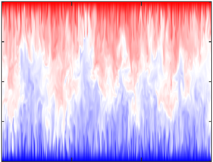
To further examine the logarithmic region, figure 5 shows the corresponding diagnostic function  $\beta =y^*(\mathrm {d} U^*/\mathrm {d} y^*)$ for the mean velocity profile under TL transformation. As the Reynolds number increases, the
  $\beta$ profiles collapse for
  $y^*$ up to
  $50$, and slowly develop a plateau with
  $\beta =1/\kappa =1/0.41$ – larger than those reported for other types of wall turbulence (Lee & Moser Reference Lee and Moser2015; Pirozzoli et al. Reference Pirozzoli, Romero, Fatica, Verzicco and Orlandi2021; Yao, Chen & Hussain Reference Yao, Chen and Hussain2022). In addition, at a common
  $Re^*_{\tau,c}$ (e.g. figure 5b), the compressible and incompressible cases agree very well. Notable differences appear between PC and PP flows (figure 5a) – akin to that found in incompressible flow by Avsarkisov et al. (Reference Avsarkisov, Hoyas, Oberlack and Garcia-Galache2014). In particular, for the
  $Re_\tau$ considered,
  $\beta$ in PC flow is much flatter than that in PP flow, which indicates that the log layer in the former is less sensitive to the Reynolds number effect. For the ILM500 case (figure 5a),
  $\beta$ starts to drop sharply at
  $y^*=200$. Such a drop, also observed for even higher
  $Re_\tau$ DNS (Pirozzoli et al. Reference Pirozzoli, Bernardini and Orlandi2014) and LES (Chen et al. Reference Chen, Lv, Xu, Shi and Yang2022) studies, is not apparent for the compressible cases considered here – presumably due to relatively low
  $Re^*_{\tau,c}$.

Figure 5. The log-law diagnostic function of the TL transformed velocities  $\beta =y^* (\mathrm {d} U^*/\mathrm {d} y^*)$ for (a) subsonic and (b) supersonic cases. Note that the IPP500 case in (a) is for incompressible PP flow at
  $Re_\tau =500$ (Yao, Chen & Hussain Reference Yao, Chen and Hussain2019), and the dash-dotted line represents
  $\beta =1/\kappa$ with
  $\kappa =0.41$.
Another important question in PC flows is the Reynolds number dependence of the velocity gradient at the channel centreline, which is defined as
 \begin{equation} \psi=\left.\frac{h}{U_w}\frac{\mathrm{d} U}{\mathrm{d} y}\right|_{y/h=0}. \end{equation}
In PP flows,  $\psi$ is always zero by symmetry, but in PC flow,
  $\psi$ is not necessarily zero as the mean velocity becomes anti-symmetric. As
  $\psi$ is directly related to turbulence production in the outer region, understanding its behaviour with increasing Reynolds number is essential and has been debated in many incompressible works. For example, based on the experimental results by Reichardt (Reference Reichardt1959), Busse (Reference Busse1970) suggested that
  $\psi$ approaches
  $0.25$ at infinite Reynolds number. However, Lund & Bush (Reference Lund and Bush1980) performed an asymptotic analysis and suggested that
  $\psi$ should approach zero as
  $Re\to \infty$. Recently, Chen et al. (Reference Chen, Lv, Xu, Shi and Yang2022) proposed that
  $\psi$ should decrease exponentially for sufficiently high Reynolds numbers.
Figure 6(a) shows the  $Re_\tau$ dependence of
  $\psi$ for different
  $M_w$ cases, along with the incompressible results of Lee & Moser (Reference Lee and Moser2018) and Avsarkisov et al. (Reference Avsarkisov, Hoyas, Oberlack and Garcia-Galache2014). The uncertainty of
  $\psi$ due to averaging over limited time samples is estimated via an autoregressive method as described in Oliver et al. (Reference Oliver, Malaya, Ulerich and Moser2014) and Rezaeiravesh et al. (Reference Rezaeiravesh, Xavier, Vinuesa, Yao, Hussain and Schlatter2022). Consistent with previous findings, at a given
  $M_w$,
  $\psi$ decreases with
  $Re_\tau$, but the Reynolds number range considered is too narrow to predict the asymptotic behaviour of
  $\psi$. There is a notable scatter among different
  $M_w$ cases, particularly at large
  $Re_\tau$, and the discrepancy is beyond the uncertainty limit. However, such scatter can be significantly reduced by plotting
  $\psi$ as a function of
  $Re^*_{\tau,c}$ (figure 6b), in which reasonably good collapses can be observed between different
  $M_w$ cases. It suggests that the scaling of
  $\psi$ should follow the incompressible situation when local flow properties are taken into consideration. The larger discrepancy for the incompressible cases among different datasets might be attributed to the domain size effect. For example, Lee & Moser (Reference Lee and Moser2018) found approximately 14 % variation in
  $\psi$ between their small and large domain cases. This is further supported by the results in Appendix B, where
  $\psi$ between different domain sizes varies about
  $16\,\%$ for
  $Re_w=4000$ and
  $M_w=1.5$ case.

Figure 6. Mean velocity gradient at the channel centreline  $\psi$ and its uncertainty as functions of (a)
  $Re_\tau$ and (b)
  $Re^*_{\tau,c}$.
3.3. Reynolds stresses
The non-zero Reynolds stresses  $\tau _{ij}=\bar {\rho }R_{ij}$ with
  $R_{ij}=\widetilde {u''_iu''_j}=\widetilde {u_iu_j}- \widetilde {u_i}\widetilde {u_j}$ are examined here. Figure 7 shows the normalized Reynolds normal stresses (
 $\tau _{11}/\tau _w$,
  $\tau _{22}/\tau _w$ and
  $\tau _{33}/\tau _w$) for subsonic (left) and supersonic (right) cases. The streamwise Reynolds stress
  $\tau _{11}/\tau _w$ increases with
  $Re_\tau$, presumably resulting from the enhanced outer large-scale structures (Marusic et al. Reference Marusic, McKeon, Monkewitz, Nagib, Smits and Sreenivasan2010). Different from PP flows,
  $\tau _{11}/\tau _w$ near the centreline strongly depends on
  $Re_\tau$ – partially due to non-zero turbulence production there. For the ILM500 case, a secondary peak of
  $\tau _{11}/\tau _w$ develops at
  $y^*\approx 200$; but such a peak has not been observed for compressible cases, perhaps due to relatively low
  $Re^*_{\tau,c}$.

Figure 7. Reynolds normal stress (non-dimensionalized by  $\tau _w$) for (a,c,e) subsonic and (b,d, f) supersonic cases: (a,b)
  $\tau _{11}$; (c,d)
  $\tau _{22}$; (e, f)
  $\tau _{33}$. The dashed line in the inset of (c) denotes
  $\tau _{22}/\tau _w=by*^4$ with
  $b=1.0\times 10^{-4}$, and the dashed line (- - - - -, red) and circles (
 $\circ$, red) in (b,d, f) denote the contribution of large-scale structures (with spanwise wavelength
  $\lambda _z\ge 2 h$) to the Reynolds stresses for C10KM15 and I8KM00, respectively.
For the subsonic cases, the locations of the inner peaks are similar in the semilocal unit, namely,  $y^*\approx 15$ – consistent with other types of wall turbulence, such as PP (Lee & Moser Reference Lee and Moser2015), pipe (Wu, Baltzer & Adrian Reference Wu, Baltzer and Adrian2012; Yao et al. Reference Yao, Rezaeiravesh, Schlatter and Hussain2023) and boundary layer (Schlatter & Örlü Reference Schlatter and Örlü2010). However, as
  $M_w$ increases, the inner peak locations seem to move closer to the wall – becoming approximately
  $13.6$ for
  $M_w=5.0$. At comparable
  $Re^*_{\tau,c}$ (figure 7b),
  $\tau _{11}/\tau _w$ for the compressible cases agrees with the incompressible cases in the outer region but is larger near the wall – a feature also found for compressible PP flows (Modesti & Pirozzoli Reference Modesti and Pirozzoli2016; Yao & Hussain Reference Yao and Hussain2020; Baranwal, Donzis & Bowersox Reference Baranwal, Donzis and Bowersox2022) and cooled supersonic/hypersonic turbulent boundary layer (Zhang et al. Reference Zhang, Duan and Choudhari2018).
Figure 8(a) further shows the inner peak value of streamwise Reynolds stress ( $\tau ^p_{11}/\tau _w$) as a function of
  $Re^*_{\tau,c}$. As expected, the
  $\tau ^p_{11}/\tau _w$ grows with
  $Re^*_{\tau,c}$ (Lozano-Durán & Jiménez Reference Lozano-Durán and Jiménez2014; Lee & Moser Reference Lee and Moser2015; Marusic, Baars & Hutchins Reference Marusic, Baars and Hutchins2017). Note that the Reynolds number scaling of
  $\tau ^p_{11}$ is still a highly debated issue in incompressible wall turbulent flows. Previously,
  $\tau ^p_{11}/\tau _w$ was assumed to increase logarithmically with
  $Re_\tau$ (Marusic & Monty Reference Marusic and Monty2019). Recently, Chen & Sreenivasan (Reference Chen and Sreenivasan2021), based on the bounded wall dissipation assumption, argued that the growth of
  $\tau ^p_{11}/\tau _w$ would eventually saturate at infinite Reynolds number. The limited number and relatively narrow range of Reynolds numbers considered here prohibit us from opining as to which scaling law better fits the data. In addition, different from
  $\psi$,
  $\tau ^p_{11}/\tau _w$ does not collapse among different
  $M_w$ cases even if the semilocal unit is employed. Similar behaviour has been recently reported in the compressible PP flows (Yao & Hussain Reference Yao and Hussain2020) and hypersonic turbulent boundary layers (Zhang et al. Reference Zhang, Duan and Choudhari2018). As explained by Foysi, Sarkar & Friedrich (Reference Foysi, Sarkar and Friedrich2004), the main reason is that due to the non-local effect between the pressure and fluid inertia, the mean density
  $\bar {\rho }$ does not preserve inner scaling and, hence, cannot yield complete collapse between compressible and incompressible cases.

Figure 8. Peak values of (a) streamwise  $\tau _{11}/\tau _w$ and (b) spanwise
  $\tau _{33}/\tau _w$ Reynolds normal stresses as a function of
  $Re^*_{\tau,c}$.
Different from  $\tau _{11}/\tau _w$, good agreements are observed for the wall-normal (
 $\tau _{22}/\tau _w$) and spanwise (
 $\tau _{33}/\tau _w$) components between incompressible and compressible cases at matching
  $Re^*_{\tau,c}$, with the exception of the region immediately adjacent to the wall. This agrees with the previous observations for compressible turbulent PP flows (Modesti & Pirozzoli Reference Modesti and Pirozzoli2016; Yao & Hussain Reference Yao and Hussain2020) and boundary layers (Duan, Beekman & Martin Reference Duan, Beekman and Martin2011; Huang, Duan & Choudhari Reference Huang, Duan and Choudhari2022). With increasing
  $Re^*_{\tau.c}$,
  $\tau _{33}/\tau _w$ increases, but
  $\tau _{22}/\tau _w$ remains nearly unchanged – distinctly different from the PP flows. From figure 8(b), it is clear that the inner peak value of spanwise Reynolds stress (
 $\tau ^p_{33}/\tau _w$) grows with
  $Re^*_{\tau,c}$. In addition, in contrast to
  $\tau ^p_{11}/\tau _w$,
  $\tau ^p_{33}/\tau _w$ is independent of
  $M_w$.
Figure 9 further shows the Reynolds shear stress ( $\tau _{12}/\tau _{w}$). It starts from zero and increases asymptotically to unity at the channel centre. Similar to
  $\tau _{22}/\tau _{w}$, there is substantial concordance between incompressible and supersonic situations at matching
  $Re^*_{\tau,c}$, except for the near-wall region. Different from the PP flow, where
  $\tau _{12}/\tau _{w}$ exhibits slow but consistent growth with Reynolds number,
  $\tau _{12}/\tau _{w}$ for PC flows collapses very well between different
  $Re^*_{\tau,c}$ cases – indicating that
  $\tau _{12}/\tau _{w}$ is nearly universal in inner scaling in PC flows.

Figure 9. Reynolds shear stress (non-dimensionalized by  $\tau _w$) for (a) subsonic and (b) supersonic cases. The dashed line in the inset of (a) denotes
  $\tau _{12}/\tau _w=cy*^3$ with
  $b=1.0\times 10^{-3}$, and the dashed lines and circles in (b) denote the contribution of large-scale structures (with spanwise wavelength
  $\lambda _z\ge 2 h$) for C10KM15 and I8KM00, respectively.
Recently, Baranwal et al. (Reference Baranwal, Donzis and Bowersox2022) found that, even if the semilocal scaling is used, the near-wall asymptotic behaviour of Reynolds stresses for compressible PP flow differs from the corresponding incompressible flow. In particular, due to the constraint of the solenoidality of the velocity field, the near-wall asymptotic behaviour exhibits the theoretical behaviour for low Mach numbers flows, e.g.  $\tau _{22}/\tau _w\sim y*^4$ (figure 7c) and
  $\tau _{12}/\tau _w\sim y*^3$ (figure 9a). However, wall-normal Reynolds stresses and Reynolds shear stress components exhibit a decrease in slope as Mach number increases due to increased dilatation effects. This is confirmed in figures 7(d) and 9(b). Therefore, in the near-wall region, flow in compressible PC becomes more anisotropic than incompressible cases.
The turbulent kinetic energy production  $P_k=-\tau _{12}\,\mathrm {d} \tilde {U}/\mathrm {d} y$ normalized by wall variables
  $\mu _w/\tau ^2_w$ is displayed in figure 10. As expected, production is mainly concentrated in the near-wall region and well collapses between different
  $Re_w$ at the same
  $M_w$. Different from PP, PC flow has non-zero production at the channel centreline, whose value decreases with increasing
  $Re_w$. Assuming
  $\mathrm {d} \tilde {U}^+/\mathrm {d} y^+ \cong \mathrm {d} {U}^+/\mathrm {d} y^+$ (as the correlation
  $\overline {\rho ' u'}$ is small), (2.1) gives
 \begin{equation} P_k={-}\frac{\mu_w}{\mu}\tau^+_{12}(1+\tau^+_{12}). \end{equation}
Based on (3.8), the maximum of  $P^+_k$ is approximately equal to
  $1/4$ for the incompressible cases, where
  $\mu _w/\mu =1$ – consistent with the results shown in figure 10. In addition, the peak occurs where the Reynolds shear stress
  $-\tau ^+_{12}$ equals the viscous stress
  $\mathrm {d}\tilde {U}^+/\mathrm {d} y^+$.

Figure 10. Turbulent kinetic energy production  $P_k=-\tau ^+_{12}\,\mathrm {d} \tilde {U}^+/\mathrm {d} y^+$ as a function of
  $y^*$ for (a) subsonic and (b) supersonic cases. The inset in (b) displays the peak production
  $P^+_k(y^*_P)$ as a function of
  $\mu _w/\mu (y^*_P)$ with the dashed line denoting
  $P^+_k(y^*_P)=(\mu _w/\mu (y^*_P))/4$.
From figure 10, the peak production decreases with increasing  $M_w$. However, the peak location
  $y^*_P$ is roughly the same for all cases in the semilocal coordinates (i.e.
  $y^*\approx 11$). In addition,
  $\tau ^+_{12}$ collapses well between different
  $M_w$ cases and is roughly equal to
  $1/2$ at
  $y^*_P\approx 11$(figure 9). Therefore, following (3.8), the peak production for the compressible cases can be estimated as
  $P^+_k(y^*_P)=(\mu _w/\mu (y^*_P))/4$ – suggesting that the decreases of
  $P^+_k$ at high
  $M_w$ are mainly due to the increase of viscosity. Table 3 lists
  $\mu (y^*_P)/\mu _w$ for different cases. It is clear that
  $\mu (y^*_P)/\mu _w$ is less sensitive to
  $Re_w$ than
  $M_w$. In addition, as shown in the inset of figure 10(b), the peak production as a function of
  $\mu (y^*_P)/\mu _w$ closely follows the prediction.
3.4. Thermodynamic variables
The mean fluid thermodynamic properties are of great importance in fully developed compressible wall turbulence. Specifically, a key to understanding them lies in the rapid wall-normal changes in  $\bar {\rho }$ and
  $\bar {T}$ due to viscous heating (Ghosh, Foysi & Friedrich Reference Ghosh, Foysi and Friedrich2010). Figure 11(a) shows the mean temperature
  $\bar {T}/T_w$ as a function of
  $y^*$. Note that for the current configuration, as the heat transfer at the wall should balance the viscous heating, the temperature at the wall should be lower than that in the flow. As a result,
  $\bar {T}/T_w$ continuously increases with
  $y^*$ and becomes roughly constant in the channel centre – consistent with the observation in isothermal compressible PP flows (Huang et al. Reference Huang, Coleman and Bradshaw1995; Yao & Hussain Reference Yao and Hussain2020). And the temperature at the centre of the channel
  $\bar {T}_c$ only weakly depends on
  $Re^*_\tau$. In particular,
  $\bar {T}_c/T_w$ is approximately
  $1.1$ for all the subsonic
  $M_w=0.8$ cases (table 3). Due to enhanced viscous heating,
  $\bar {T}/T_w$ increases with
  $M_w$ notably. For example,
  $\bar {T}_c/T_w$ increases to
  $2.39$ and
  $4.84$ for
  $M_w=3$ and
  $5$, respectively. Correspondingly, the mean density
  $\bar {\rho }/\rho _w$ has its maximum at the wall and rapidly decreases with increasing
  $y$, particularly for the C4KM50 case (figure 11c). In addition,
  $\bar {\rho }/\rho _w$ reaches a plateau near the channel centre – indicating the flow is mostly incompressible in the core. Its value, which only mildly varies with
  $Re_w$, progressively decreases with increasing
  $M_w$.

Figure 11. Mean temperature  $\bar {T}$ normalized by (a) wall temperature
  $T_w$ and (b) friction temperature
  $T_\tau$ as a function of
  $y^*$; mean density
  $\bar {\rho }$ normalized by wall density
  $\rho _w$ as a function of
  $y/h$, and temperature fluctuations
  $\overline {T'^2}/T^2_\tau$ as a function of
  $y^*$. The inset in (d) is the root-mean-square (r.m.s.) of the temperature fluctuations normalized by the wall temperature
  $\sqrt {\overline {T'^2}}/T_w$.
Figure 11(b) shows  $(\bar {T}-T_w)/T_\tau$ as a function of
  $y^*$. Here,
 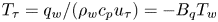 $T_\tau =q_w/(\rho _wc_pu_\tau )=-B_qT_w$ is the friction temperature. While the agreement between different
  $M_w$ is improved in the near-wall region, notable differences can be observed, particularly for the
  $M_w=5$ case – confirming the previous claim that the mean thermodynamic properties, such as
  $\bar {\rho }$,
  $\bar {T}$ and
  $\bar {\mu }$, do not preserve inner scaling.
Figure 11(d) shows the temperature fluctuations  $\overline {T'^2}$ (normalized by
  $T^2_\tau$) as a function of
  $y^*$. For a given
  $Re_w$,
  $\overline {T'^2}/T^2_\tau$ collapses between different
  $M_w$ in the outer region. Consistent with
  $\tau _{11}/\tau _w$,
  $\overline {T'}^2/T^2_\tau$ increases with both
  $Re^*_\tau$ and
  $M_w$ in the near-wall region. In addition, the location of the peak, which remain almost unchanged with
  $M_w$, shifts towards large
  $y^*$ at high
  $Re^*_\tau$. While the peak value of root-mean-square (r.m.s.) temperature fluctuations
  $\sqrt {\overline {T'^2}}$ is negligible (within
  $1\,\%$ of
  $T_w$) for
  $M_w=0.8$ cases, it strongly increases with
  $M_w$ – becoming approximately
  $21\,\%$ and
  $57\,\%$ for
  $M_w=3$ and
  $5$ cases, respectively. This suggests that the fluctuations of thermodynamic properties become progressively important at high
  $M_w$.
The mean temperature can be used to determine the mean velocity profiles and the relation between heat transfer and skin friction coefficients. Here, we provide an assessment of various velocity–temperature relationships in compressible PC flows (Walz Reference Walz1969; Duan et al. Reference Duan, Beekman and Martin2011; Zhang et al. Reference Zhang, Bi, Hussain and She2014), which can be written as
 \begin{equation} \frac{T}{T_w}=1+\alpha_1\frac{U}{U_w}+\alpha_2 \left(\frac{U}{U_w}\right)^2, \end{equation}
with parameters  $\alpha _1$ and
  $\alpha _2$ vary for different scaling relations. Note that different from PP flow, where the centreline velocity is used,
  $U_w$ is employed here for the velocity normalization. For the Walz relation,
 \begin{equation} \alpha_1=\frac{T_r-T_w}{T_w}, \quad \alpha_2={-}r\frac{\gamma-1}{2}M^2_c \frac{T_c}{T_wU^2_w}. \end{equation}
Here,  $r=Pr^{1/3}=0.89$ is the recovery factor and
  $T_r=T_c[1+(\gamma -1)rM^2_c/2]$ is the recovery temperature. Similar to the VD transformation for the mean velocity, the Walz relation and DNS are in good agreement for the boundary layer over an adiabatic wall (Pirozzoli, Grasso & Gatski Reference Pirozzoli, Grasso and Gatski2004), but have clear differences for diabatic cases (Duan et al. Reference Duan, Beekman and Martin2010).
Zhang et al. (Reference Zhang, Bi, Hussain and She2014) later derived a generalized Reynolds analogy
 \begin{equation} \alpha_1=\frac{T_{rg}-T_w}{T_w},\quad \alpha_2=\frac{T_c-T_{rg}}{T_w}, \end{equation}
with  $r_g=2C_p(T_w-T_c)/U^2_w-2Prq_w/(U_w\tau _w)$ the so-called general recovery factor and
  $T_{rg}=T_c+r_gU^2_w/(2C_p)$.
Figure 12(a) compares the DNS data with these velocity–temperature relations. Equation (3.11a,b) provides a better fit than (3.10a,b) – similar to the findings in the compressible PP flow (Yao & Hussain Reference Yao and Hussain2020) and the cooled turbulent boundary layer (Zhang et al. Reference Zhang, Duan and Choudhari2018; Chen et al. Reference Chen, Lv, Xu, Shi and Yang2022). Note that in PP flows, these relations cannot be explicitly employed to derive the mean velocity as the centreline values of mean velocity and temperature are not known a priori. However, such issues can be overcome for PC flows if  $T_c$ can somehow be estimated (as
  $U_w$ is fixed for all cases).

Figure 12. (a) Mean temperature ( $T/T_w$) as a function of mean velocity
  $U/U_w$ for C10KM08, C10KM15 and C4KM50, compared with (3.10a,b) (dashed-dotted line), (3.11a,b) (dashed line) and (3.11a,b) with
  $T_c$ estimated based on (3.12)(dotted); and (b) the temperature at the centreline (
 $T_c/T_w$) as a function of
  $M_w$ and (b). Note that the solid line in (b) denotes the relation (3.12) with
  $r_c=0.783$.
Recently, an empirical scaling for  $T_c$ in compressible PP flows with symmetric isothermal boundary conditions was proposed by Song et al. (Reference Song, Zhang, Liu and Xia2022), and it can be extended to PC flows as
 \begin{equation} \frac{T_c}{T_w}=1+r_c\frac{\gamma-1}{2}M^2_w, \end{equation}
with  $r_c$ the recovery factor for the mean temperature at the channel centreline.
Figure 12(b) shows the  $T_c/T_w$ as a function of
  $M_w$. It is clear that the scaling (3.12) with
  $r_c=0.783$ obtained from fitting the DNS data proves to be a very good estimation of
  $T_c/T_w$. Figure 12(a) further confirms that (3.11a,b) in combination with (3.12) also produces an excellent correlation between mean velocity and temperature.
The turbulent heat flux is essential for modelling compressible flows. Figure 13 shows streamwise  $\bar {\rho }\widetilde {u''T''}$ and wall-normal
  $\bar {\rho }\widetilde {v''T''}$ components of turbulent heat flux (normalized by
  $\rho _w u_\tau T_\tau$) as a function of
  $y^*$. Note that the
 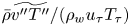 $\bar {\rho }\widetilde {v''T''}/(\rho _w u_\tau T_\tau )$ has a much smaller magnitude than
  $\bar {\rho }\widetilde {u''T''}/(\rho _w u_\tau T_\tau )$, and, in contrast with the Reynolds shear stress, it does not have a universal profile. For both quantities, there is a notable increase in the peak magnitude with increasing
  $Re^*_{\tau,c}$, and the corresponding peak location also shifts away from the wall. With increasing
  $M_w$,
  $\bar {\rho }\widetilde {u''T''}$ at a given
  $Re_w$ increases/decreases in the near-wall/outer regions, respectively. But,
  $\bar {\rho }\widetilde {v''T''}$ decreases with increasing
  $M_w$ in the whole range of
  $y$. Such discrepancy between different
  $M_w$ cases is partially attributed to the slight difference in
  $Re^*_{\tau,c}$.

Figure 13. Streamwise  $\bar {\rho }\widetilde {u''T''}/(\rho _w u_\tau T_\tau )$ and wall-normal
  $\bar {\rho }\widetilde {v''T''}/(\rho _w u_\tau T_\tau )$ components of turbulent heat flux as a function of
  $y^*$.
3.5. Energy spectra
Energy spectra, which illustrate how the kinetic energy of turbulence is dispersed across different scales, have been extensively utilized to get a deeper comprehension of the turbulence cascade (Jiménez Reference Jiménez2012). Figures 14 and 15, respectively, show the premultiplied streamwise spectra  $k_x E_{\rho uu}/\tau _w$ and
  $k_x E_{\rho uv}/\tau _w$ as a function of
  $\lambda _x/h$ and
  $y^*$. Note that following Patel et al. (Reference Patel, Peeters, Boersma and Pecnik2015), the spectrum is computed for the velocity fluctuation weighted by the local density so that the premultiplied spectra represent its contribution to the intensity of the Reynolds stresses. It has been established previously that semilocal scaling can result in a superior collapse compared with wall unit scaling (Yao & Hussain Reference Yao and Hussain2019). The
  $k_x E_{\rho uu}/\tau _w$ spectra clearly show the presence of an energetic inner peak at
  $y^*\approx 13$ – corresponding to the near-wall self-sustaining regenerative cycle (Waleffe Reference Waleffe1997; Schoppa & Hussain Reference Schoppa and Hussain2002). For a given
  $M_w$, the streamwise wavelength in physical unit
  $\lambda _x/h$ decreases with increasing
  $Re_\tau$, but remains roughly the same in semilocal units
  $\lambda ^*_x\approx 1000$, which represents the average length of near-wall streaks. Figure 16(a) compares
  $k_x E_{\rho uu}/\tau _w$ as a function of
  $\lambda ^*_x$ between C10KM15 and I8KM00 cases. Although the length scales do not vary with
  $M_w$, the magnitudes of the inner peak increase with
  $M_w$ – consistent with the larger
  $\tau _{11}/\tau _w$ in figure 7(a,b).

Figure 14. Premultiplied streamwise spectra of streamwise velocity  $k_x E_{\rho uu}/\tau _w$.

Figure 15. Premultiplied streamwise spectra of Reynolds shear stress  $k_x E_{\rho uv}/\tau _w$.

Figure 16. One-dimensional premultiplied spectra of streamwise velocity  $k E_{\rho uu}/\tau _w$ at different wall-normal locations as functions of (a)
  $\lambda ^*_x$ and (b)
  $\lambda ^*_z$ for C10KM15 and I8KM00 cases.
Another notable difference between different  $M_w$ cases is the energy content near the channel centre. The energy at large wavelengths is enhanced with increasing
  $M_w$, particularly for higher
  $Re^*_{\tau,c}$. Note that such an increase in the energy content at large
  $\lambda _x/h$ does not imply that the large-scale structures at high
  $M_w$ are stronger than those in incompressible case but rather that they are less uniform in the streamwise direction, as depicted in the flow visualization in § 3.6. The
  $k_x E_{\rho uv}/\tau _w$ spectra (figure 15) have similar features to
  $k_x E_{\rho uu}/\tau _w$, except that the inner peak is located at smaller
  $\lambda _x/h$ and higher
  $y^*$. In addition, the magnitude of the inner peak is less sensitive to
  $M_w$ and
  $Re^*_{\tau,c}$ – consistent with that observed for the Reynolds shear stress
  $\tau _{12}/\tau _w$ profiles in figure 9.
Figures 17 and 18 display the premultiplied spanwise spectra  $k_z E_{\rho uu}/\tau _w$ and
  $k_z E_{\rho uv}/\tau _w$, respectively. First, a distinct low wavelength peak in
  $k_z E_{\rho uu}/\tau _w$ occurs near the wall. For both the incompressible and compressible cases, the typical length scale of the peak remains nearly universal in semilocal units, namely,
  $\lambda ^*_z\simeq 110$. A salient feature of the PC flow is the pronounced peak at large spanwise wavelengths. This peak has its maximum magnitude at the centreline and spans almost the whole channel (i.e. until
  $y^*\approx 5$). It results from the large-scale streamwise rollers inherent to PC flow, whose strength increases with the Reynolds number (Komminaho et al. Reference Komminaho, Lundbladh and Johansson1996; Tsukahara et al. Reference Tsukahara, Kawamura and Shingai2006). Different from the
  $k_x E_{\rho uu}/\tau _w$, good agreements of
  $k_z E_{\rho uu}/\tau _w$ can be observed between the compressible and incompressible cases at comparable
  $Re^*_{\tau,c}$ (see figure 16b) – suggesting that these large-scale structures have similar features in the spanwise direction. The spanwise scale of the outer peak is approximately
  $\lambda _z/h\sim 1.5{\rm \pi}$, which is one quarter of our spanwise domain – similar to the previous observations by Avsarkisov et al. (Reference Avsarkisov, Hoyas, Oberlack and Garcia-Galache2014) and Lee & Moser (Reference Lee and Moser2018). In addition, for a given
  $Re_w$, the magnitude of the peak decreases with increasing
  $M_w$ – consistent with a decrease in
  $Re^*_{\tau,c}$. Note that in the PP flow, a distinct outer peak is not observed until
  $Re_\tau > 5000$ (Lee & Moser Reference Lee and Moser2015), and it is with a much smaller spanwise length scale (i.e.
  $\lambda _z\sim h$) and does not extend that close to the wall.

Figure 17. Premultiplied spanwise spectra of streamwise velocity  $k_z E_{\rho uu}/\tau _w$.

Figure 18. Premultiplied spanwise spectra of Reynolds shear stress  $k_z E_{\rho uv}/\tau _w$.
The  $k_z E_{\rho uv}/\tau _w$ spectra are quite similar to
  $k_z E_{\rho uu}/\tau _w$, but the sharp peak at large spanwise wavelengths does not extend that near to the wall. The contributions of large-scale structures (defined with scales that with spanwise wavelength
  $\lambda _z\ge 0.5{\rm \pi} h$) to the Reynolds stresses are further shown in figures 7 and 9 for C10KM15 and I8KM00 cases. They progressively increase with
  $y$ and achieve their maximum near channel centreline (e.g. approximately
  $40\,\%$ of the total Reynolds shear stress at
  $y/h=0$).
3.6. Instantaneous turbulence structures
Figure 19 visualizes the instantaneous streamwise velocity field in the  $x$–
$x$– $z$ plane at the channel centreline (i.e.
  $y/h=0$). For all cases, there are well-defined streaks that alternate in sign along the spanwise direction. For a given
  $M_w$, the streaks undergo strong meandering along the streamwise directions at low
  $Re^*_{\tau,c}$ and become stronger and more streamwise uniform as
  $Re^*_{\tau,c}$ increases (e.g. see the middle column for C2KM15, C4KM15 and C10KM15 cases). This is consistent with the finding by Lee & Moser (Reference Lee and Moser2018) that the coherence of the streaks significantly increases with Reynolds number, and, eventually, the large-scale meandering becomes too small to be identified even with a relatively large simulation domain (e.g.
  $L_x=100{\rm \pi} h$). And for a given
  $Re^*_{\tau,c}$ case, the streaks for the compressible cases are less organized/coherent in streamwise direction than in incompressible cases – akin to the observation by Buell (Reference Buell1991). For example, the streaks for the incompressible I8KM00 case become almost streamwise uniform but remain wavy for the supersonic C10KM15 case, which are responsible for the strong energy content at large wavelengths in the streamwise spectrum (figure 14). This finding is also consistent with the instability analysis by Malik, Alam & Dey (Reference Malik, Alam and Dey2006), who found that the most unstable streamwise wavenumber increases with
  $M_w$.

Figure 19. Instantaneous streamwise velocity in  $x-z$ plane at the channel centreline (i.e.
  $y/h=0$).
Figure 20 shows a snapshot of the instantaneous streamwise velocity in a cross-stream ( $y$–
$y$– $z$) plane for the I8KM00 and C10KM15 cases. First, numerous small-scale streaks appear near both walls, and their sizes in the physical unit are comparable between these two cases. Furthermore, there also exist large-scale streaks, with the spanwise length scale comparable to the channel height. For the I8KM00 case, the large-scale streaks extend beyond the centreline, reaching very close to the opposite wall. This effect is less apparent for the C10KM15 case – mainly due to the density stratification caused by the wall cooling. Since the spanwise wavelength remains the same, the flank angles of the large-scale streaks become smaller for the compressible case – affecting the generation of large-scale streamwise vortices via instability/transient growth (Waleffe Reference Waleffe1997; Schoppa & Hussain Reference Schoppa and Hussain2002).

Figure 20. Comparison of instantaneous streamwise velocity in a cross-stream ( $y$–
$y$– $z$) plane for (a) I8KM00 and (b) C10KM15 cases.
Figure 21 further shows the vortical structures in the bottom half-channel (i.e.  $-1\le y\le 0$) together with the streamwise velocity fluctuations (
 $u'/U_w$) at
  $y^*=15$. Note that the vortices are visualized using the isosurfaces of
  $\lambda _\rho$ criterion (Yao & Hussain Reference Yao and Hussain2018). The distributions of
  $\lambda _\rho$ structures are quite similar between the I8KM00 and C10KM15 cases. While the buffer layer is dominated by quasi-streamwise vortices, the log and outer regions exhibit a few hairpin-like vortices. Furthermore, the footprint of large-scale streaks influences the strengths of these vortical structures. Specifically, they are stronger/weaker in the vicinity of large-scale high-speed/low-speed regions, respectively – consistent with the observation of previous studies (Ganapathisubramani et al. Reference Ganapathisubramani, Hutchins, Monty, Chung and Marusic2012; Hwang & Sung Reference Hwang and Sung2017).

Figure 21. Instantaneous  $\lambda _\rho$ vortical structures shaded with the streamwise velocity
  $u$ for (a) I8KM00 and (b) C10KM15 cases. Note that the grey colour denotes the streamwise velocity fluctuations
  $u'/U_w$ at
  $y^*=15$.
3.7. Large-scale streamwise rollers
Considering that streamwise coherence exists throughout the entire streamwise computational domain, we further compare the time evolution of streamwise-averaged velocity  $\langle u \rangle _x$ at the channel centreline for I8KM00 and C10KM15 cases (figure 22a). Similar to the findings in Lee & Moser (Reference Lee and Moser2018),
  $\langle u \rangle _x$ for the I8KM00 case also appears to be coherent in time with no significant spanwise drift over time. This suggests that a more comprehensive representation of the large-scale structures can be obtained through further temporal averaging. Figure 22(b) shows the corresponding streamwise- and time-averaged streamwise velocity
  $\langle u \rangle _{x,t}$ and streamfunction in the cross-stream (
 $y$–
$y$– $z$) plane. The structures are composed of pairs of counter-rotating streamwise rollers that occupy the entire region between the two walls. Note that due to the periodic boundary condition employed, the separation distance between these counter-rotating rollers
  $\Delta z_r$ slightly depends on the spanwise domain size. For example,
  $\Delta z_r$ is
  $L_z/4$(
 $=1.5{\rm \pi} h$) in our case but is
  $\Delta z_r=5{\rm \pi} /3$ in Lee & Moser (Reference Lee and Moser2018). As the streamwise velocity for compressible cases is meandering in the streamwise direction,
  $\langle u \rangle _x$ has a relatively smaller amplitude than in incompressible cases. Furthermore, it is also less coherent in time, particularly for the C10KM15 case. Consequently, compared with the I8KM00 case, the streamwise and temporal averaged large-scale structures are less organized.

Figure 22. (a) Time evolution of streamwise velocity  $u$ averaged in streamwise direction at the channel centreline as a function of
  $z$; (b) streamwise- and temporal-averaged streamwise velocity and the streamfunction with solid and dashed lines denoting the positive and negative values, respectively.
The two-point auto-correlation of the streamwise velocity is employed to probe the nature of the large-scale structures quantitatively
 \begin{equation} R_{uu}(r_x,r_z,y,y_{r})=\frac{\langle{u'(x_r,y_{r},z_r) u'(x+r_x,y,z+r_z)}\rangle}{\langle{u'^2}\rangle^{1/2}(y) \langle{u'^2}\rangle^{1/2}(y_{r})}, \end{equation}
where  $(x_r,y_r,z_r)$ is the reference point, and
  $r_x$ and
  $r_z$ are the separation distances in the
  $x$- and
  $z$-directions, respectively.
Figure 23 displays the two-point auto-correlation of the streamwise velocity at the centreline  $R_{uu}(r_x,r_z,0,0)$ for I8KM00 and C10KM15 cases. First, there is a regular alternation in the sign of
  $R_{uu}(r_x,r_z,0,0)$ in the spanwise direction, with a wavelength
  $\lambda _z/h=1.5{\rm \pi}$, which does not vary with
  $M_w$ – consistent with the presence of the prominent peaks in the spanwise energy spectra in figure 17. As observed by Lee & Moser (Reference Lee and Moser2018), the correlation coefficients for the I8KM00 case do not alter the sign over the entire streamwise direction – indicating that the computational domain size employed is not sufficient for capturing one streamwise wavelength of the large-scale structures. With increasing
  $M_w$,
  $R_{uu}(r_x,0,0,0)$ drops much faster and changes the sign for the C10KM15 case. The location for
  $R_{uu}(r_x,0,0,0)$ to be zero becomes shorter with higher
  $M_w$. It implies that the streamwise wavelength of the dominant large-scale structures decreases with increasing
  $M_w$. A much longer streamwise domain size would obviously be required to measure the exact length scale.

Figure 23. Two-point correlations of streamwise velocity  $R_{uu}(r_x,r_z,0,0)$ in the
  $x$–
$x$– $z$ plane at the channel centreline.
Figures 24(a) and 24(b), respectively, show the contour plots of the two-point auto-correlation of the streamwise velocity in the ( $x$–
$x$– $y$) and (
 $x$–
$x$– $z$) planes for the C10KM15 case. Note that the reference point is chosen to be in the channel centre (i.e.
  $y_r=0$), and the dashed lines denote the results for the I8KM00 case. Consistent with the energy spectra, the structures fill in the whole domain between the two moving walls. The distribution of
  $R_{uu}(r_x,0,y,0)$ are leading (top wall) and trailing (bottom wall) with respect to the centreline. In addition, the negative correlation appears in a wide region of
  $r_x>6{\rm \pi} h$. Note that the negative region is not observed for the I8KM00 case – consistent with the results shown in figure 19 that the streaks are almost streamwise uniform. The distribution of
  $R_{uu}(0,r_z,y,0)$ reveals the existence of organized pairs of counter-rotating streamwise rollers, which share similar characteristics between the C10KM15 and C8KM00 cases.

Figure 24. Two-point correlations of streamwise velocity (a)  $R_{uu}(r_x,0,y,0)$ and (b)
  $R_{uu}(0,r_z,y,0)$ for the C10KM15 case. The black dashed line is for the I8KM00 case.
3.8. Amplitude modulation
The modulating effect of outer large-scale streamwise rollers on the near-wall small-scale structures is further investigated here. This was first studied by Bandyopadhyay & Hussain (Reference Bandyopadhyay and Hussain1984) and later extended by Mathis, Hutchins & Marusic (Reference Mathis, Hutchins and Marusic2009) by introducing a single-point correlation coefficient
 \begin{equation} R_{AM}(y^+)=\frac{\overline{u^+_L E_L(u^+_S)}}{\sqrt{\overline{u^{{+}2}_L}}\sqrt{\overline{E_L(u^+_S)^2}}}, \end{equation}
where  $\sqrt {\overline {u^{+2}_L}}$ and
  $\sqrt {\overline {E_L(u^+_S)^2}}$ denote the r.m.s. of the large-scale signal
  $u^+_L$ and the filtered envelope of small-scale signal
  $E_L(u^+_S)$. Note that
  $E_L(u^+_S)$ is obtained by applying Hilbert transform to the small-scale component
  $u^+_S$ and then low-passed filtered at the same cutoff wavelength as the large-scale component. When considering amplitude modulation, it typically requires at least information at two different wall-normal locations, hence the two-point correlations. However, Mathis et al. (Reference Mathis, Hutchins and Marusic2009) showed that the one-point correlation
  $R_{AM}$ provided a fair estimation of the degree of modulation when compared with the ideal two-point coefficient. The reason is that the large scales in the outer region affect the near-wall small scales through direct penetration; hence, they have their footprint in the near wall, which is evident from the premultiplied energy spectra (figure 17) and instantaneous flow visualization (figure 21).
Following Dogan et al. (Reference Dogan, Örlü, Gatti, Vinuesa and Schlatter2019), we employ the two-dimensional spectral filter to separate the velocity filed into large and small scales. In particular, the small scales are defined as those with wavelengths smaller than the cutoffs both in the streamwise and spanwise directions. Regarding the cutoffs,  $\lambda _x/h\approx 2{\rm \pi}$ and
  $\lambda _z/\delta \approx 0.5{\rm \pi}$ are used, which, based on inspection of the spectra (figures 16 and 17), represent the boundary between the large and small scales. (Note that altering the filter size revealed no qualitative difference is noticed.)
Figure 25 shows the one-point amplitude modulation coefficient  $R_{AM}$ as a function of
  $y^*$. For comparison, results from PP flows at
  $Re_\tau =380$ (Yao & Hussain Reference Yao and Hussain2020) and from turbulent boundary layer at
  $Re_\tau \approx 3000$ (Mathis et al. Reference Mathis, Hutchins and Marusic2009) are also included. A large
  $R_{AM}$ (i.e. 0.6) in the viscous sublayer suggests a high level of modulation of the near-wall small scales by the large scales, presumably the streamwise rollers. This effect is of major significance regarding the roles and large-scale and very-large-scale motions as their footprints interact (via both sweep and shear) with near-wall, small-scale structures. The value of
  $R_{AM}$ decreases to approximately zero in the log region and becomes negative in the outer region. Furthermore,
  $R_{AM}$ between the I8KM00 and C10KM15 cases collapse very well across the whole wall-normal range. This shows that the modulation effect between incompressible and compressible cases is quite similar when the semilocal Reynolds numbers at the channel centreline
  $Re^*_{\tau,c}$ are equal. In addition,
  $R_{AM}$ in PC flows is much stronger than in PP flows at comparable
  $Re_\tau$ and is nearly comparable to turbulent boundary layer at much higher
  $Re_\tau$ (i.e.
  $\approx 3000$). Therefore, PC flow can be employed to better explore the physics and control of the large- and small-scale interactions – without the need for extremely high Reynolds numbers (Pirozzoli, Bernardini & Orlandi Reference Pirozzoli, Bernardini and Orlandi2011).

Figure 25. Distribution of the one-point amplitude modulation coefficient  $R_{AM}$ for C10KM15 andI8KM00 cases.
4. Concluding remarks
Direct numerical simulations of compressible turbulent PC flows are conducted for  $Re_w=1500$,
  $4000$ and
  $10\ 000$ with the highest
  $M_w$ up to
  $5$. While
  $C_f$ decreases with
  $Re_w$, it only weakly depends on
  $M_w$. In addition, the thermodynamic properties (e.g. mean temperature, density, etc.) strongly vary with
  $M_w$. Consistent with prior research on other types of wall turbulence, the compressibility effects on most turbulent statistics can be well incorporated by using the semilocal scaling based on the local mean viscosity and density. In particular, the mean velocity profiles under TL transformation (Trettel & Larsson Reference Trettel and Larsson2016) collapse very well with the incompressible ones at comparable
  $Re^*_{\tau,c}$ and develop a logarithmic layer that extends closer to the channel centreline with a Kárman constant
  $\kappa =0.41$. Reynolds stresses exhibit the same behaviours as incompressible flows, including peak locations and magnitudes. The inner peak of the streamwise Reynolds stress for PC increases with
  $M_w$, which is consistent with the findings for compressible PP flows. In addition, due to rapid wall-normal changes of viscosity caused by viscous heating, the turbulent production in the near-wall region decreases as
  $M_w$ increases, and its peak, when scaled in wall units, follows
  $P^+_k(y^*_P)=(\mu _w/\mu (y^*_P))/4$, where
  $y^*_P(\approx 11)$ is the peak location in semilocal units.
The one-dimensional streamwise and spanwise premultiplied velocity spectra are also examined. The streamwise velocity spectra show a distinct inner peak located at  $\lambda ^*_x\approx 1000$ and
  $\lambda ^*_z\approx 110$ – indicating that the near-wall structures are universal for all types of wall turbulence. In addition, the spanwise spectra display an outer peak located at
  $\lambda _z/h\approx 1.5h$. This peak has its maximum magnitude at the centreline and spans over the whole channel depth (i.e. until approximately
  $y^*=5$) – resulting from the large-scale streamwise structures specific to PC flows. The characteristics of these structures are examined by flow visualization. For strictly incompressible cases, the structures are comprised pairs of streamwise-uniform, counter-rotating rollers that occupy the entire region between the two parallel walls. As
  $M_w$ increases, the large-scale structures become less organized/coherent in the streamwise direction. The two-point auto-correlation further confirms that the streamwise length scale of these structures decreases with increasing
  $M_w$. The reason for this still needs further investigation. The amplitude modulation of near-wall small-scale structures by the large-scale streamwise rollers is also studied. A high level of modulation of large scales on small scales is observed close to the wall. In addition, the modulation effect is quite similar between incompressible and compressible cases at similar
  $Re^*_{\tau,c}$ – but much stronger than in PP flows.
Acknowledgements
We appreciate M. Lee and R. Moser for providing us with their incompressible DNS code used for this study.
Funding
Computational and visualization resources provided by Texas Tech University HPCC, TACC Lonestar, Stampede2 and Frontera are acknowledged.
Declaration of interests
The authors report no conflict of interest.
Data availability statement
The data that support the findings of this study are openly available at https://dataverse.tdl.org/dataverse/ctpcf.
Appendix A. Validation of numerical solver for PC flow at low Mach number
The solver has been extensively validated in our previous works (Yao & Hussain Reference Yao and Hussain2019, Reference Yao and Hussain2020) for the PP configuration by comparing flow statistics with both the incompressible dataset of Lee & Moser (Reference Lee and Moser2015) and the compressible dataset of Modesti & Pirozzoli (Reference Modesti and Pirozzoli2016). The solver is validated here for the compressible PC flow at  $Re_w=1500$ in the nearly incompressible region (i.e.
  $M_w=0.2$) and compared with the strictly incompressible data of Lee & Moser (Reference Lee and Moser2018). The domain size and the corresponding number of grid points are the same as in the C2KM08 and C2KM15 cases, which results in mesh resolutions of
  $\Delta x^+=9.2$,
  $\Delta y^+_w=0.22$,
  $\Delta y^+_c= 2.99$ and
  $\Delta z^+=4.6$. Figure 26 shows the profiles of mean velocity (
 $U^+$) and Reynolds stresses (
 $\tau ^+_{ij}$). Excellent agreement is observed, except for minor differences near the peak and centre of
  $\tau ^+_{11}$.

Figure 26. (a) Mean velocity ( $U^+$) and (b) velocity variances and covariance for the case with
  $Re_w=1500$ and
  $M_w=0.2$. Solid lines and circles, respectively, represent results from our DNS and from Lee & Moser (Reference Lee and Moser2018) at
  $Re_\tau =93$.
Appendix B. Domain size effect for compressible PC flow
Numerical simulations of PC flow with periodic boundary conditions are known to be highly sensitive to the computational domain size – potentially leading to artificial confinement effects (Komminaho et al. Reference Komminaho, Lundbladh and Johansson1996; Pirozzoli et al. Reference Pirozzoli, Bernardini and Orlandi2014). The effect of the domain size on flow physics is further examined by performing additional DNSs with various streamwise and spanwise lengths at  $Re_w=4000$ and
  $M_w=1.5$. The details of domain sizes, grid sizes and resolutions are listed in table 4.
Table 4. Summary of the simulation parameters for different domain size cases with  $Re_w=4000$ and
  $M_w=1.5$. Here,
  $\psi$ is the velocity gradient at the channel centreline.

Figure 27(a) shows the mean velocity profiles based on the TL transformation as a function of  $y^*$. While the agreement between different cases is good in the near-wall region, notable discrepancies are observed near the channel centreline. Compared with the C4KM15 case, the velocity gradient at the channel centreline
  $\psi$ for the C4KM15S case is increased by approximately 16 % (table 4). This suggests that the larger discrepancy in
  $\psi$ results from the domain size effect, particularly in the streamwise direction. Figure 27(b) shows the Reynolds normal and shear stresses as a function of
  $y^*$. Interestingly,
  $\tau _{11}/\tau _w$ is the only component that exhibits certain disagreement. Specifically,
  $\tau _{11}/\tau _w$ for the C4KM15S case is slightly smaller than in other cases, particularly in the outer regions. It confirms that the domain size employed in the main text is sufficient to yield good statistics. Figure 28 shows the two-point auto-correlation of the streamwise velocity at the centreline
  $R_{uu}(r_x,r_z,0,0)$ for different domain size cases. Consistent with figure 23, a regular alternation in the sign of
  $R_{uu}(r_x,r_z,0,0)$ in the spanwise direction exists, and the wavelength is the same between different cases; namely,
  $\lambda _z/h=1.5{\rm \pi}$. This confirms that the characteristics of the large-scale spanwise roller is not very sensitive to the spanwise domain size. The correlation coefficients for the C4KM15S case do not alter sign across the entire streamwise direction. In particular, the correlation falls to
  $0.15$ at
  $r_x/h=L_x/2$ and
  $r_z=0$ – indicating that the streamwise computational domain size (i.e.
  $L_x=12{\rm \pi}$) is not sufficient for capturing one streamwise wavelength of the large-scale structures. With increasing
  $L_x$,
  $R_{uu}(r_x,0,0,0)$ does change sign. It is approximately
  $r_x/h\approx 6{\rm \pi}$ for the C4KM15M case – consistent with the observation in figure 23 for the C10KM15 case.

Figure 27. (a) The TL transformed mean velocity profiles transformed and (b) Reynolds stresses for different domain sizes with  $Re_w=4000$ and
  $M_w=1.5$. The dashed and dash-dotted lines in (a) denote
  $U^{\ast}=y^{\ast}$ and log law
  $U^{\ast}=(1/\kappa )\ln y^{\ast}+B$, where
  $\kappa =0.41$ and
  $B=5.2$.

Figure 28. Two-point correlations of streamwise velocity  $R_{uu}(r_x,r_z,0,0)$ in a wall-parallel (
 $x$–
$x$– $z$) plane at the channel centreline for different domain sizes with
  $Re_w=4000$ and
  $M_w=1.5$.


 Open access