

Introduction
Overview of REE patterns
The series of elements from La through to Lu are known as the lanthanides. Under typical geological conditions they occur as trivalent cations with the exception of Ce (also often tetravalent) and Eu (often also divalent). Their valence electron structures are similar, and cationic radii vary quadratically from the large La3+ to the small Lu3+ due to the lanthanide contraction (Raymond et al., Reference Raymond, Wellman, Sgarlata and Hill2010; Seitz et al., Reference Seitz, Oliver and Raymond2007). This contraction, together with its effect on mesoscale molecular interactions (Ferru et al., Reference Ferru, Reinhart, Bera, Olvera de la Cruz, Qiao and Ellis2016) leads to small yet gradual and predictable changes in their chemical behaviour. Yttrium is positioned above the lanthanides in group 3 of the periodic table, and it often behaves like Dy or Ho, particularly in high-temperature igneous or metamorphic environments (Pack et al., Reference Pack, Russell, Shelley and van Zuilen2007). The lanthanides and Y, excluding the unstable Pm (whose natural abundance is negligible, Kuroda, Reference Kuroda1982), are often grouped together as the rare earth elements (REE: Balaram, Reference Balaram2019; Cheisson and Schelter, Reference Cheisson and Schelter2019). Subsets of the REE group that commonly occur together in various rocks and minerals are termed as the light REE (LREE), heavy REE (HREE), and less commonly, the middle REE (MREE), with the exact boundaries between the subsets varying between authors. Often, the LREE group includes La to Sm, whereas the HREE group includes Eu to Lu. The MREE group, when used, typically includes Sm to Dy. The smooth variation in the chemical properties between the REE allows systematic fractionation from each other, and studies into these processes provide windows into a variety of geochemical and cosmochemical processes.
Although differences between the REE chemical properties are gradual, the variation in their natural abundances is not. They follow the Oddo–Harkins rule, which states that elements with even atomic numbers (e.g. Dy) are more abundant than their neighbouring odd-numbered elements (e.g. Tb and Ho) (Harkins, Reference Harkins1917; Palme et al., Reference Palme, Lodders, Jones and Davis2014). This complicates comparison of subtle differences between rocks or minerals because of the characteristic zig-zag shape of REE abundance plots (Taylor, Reference Taylor1962). The difficulty is resolved by normalisation to REE contents of a representative primitive or primordial reservoir, most commonly CI chondrites (Coryell et al., Reference Coryell, Chase and Winchester1963). When plotted in a logarithmic scale, the normalisation results in generally smooth REE patterns in which fractionation trends become obvious, facilitating the use of REE patterns as petrogenetic tools.
A practical limitation stems from the appearance of each analysis as a line on REE plots, which convolutes studies of large analytical data sets owing to visual overload. O'Neill (Reference O'Neill2016) developed a method to represent REE patterns by the polynomial:
 $$\ln \left({\displaystyle{{\lsqb {{\rm REE}} \rsqb } \over {{\lsqb {{\rm REE}} \rsqb }_{{\rm CI}}}}} \right) = {\rm \lambda }_0 + {\rm \lambda }_1{\rm f}_1 + {\rm \lambda }_2{\rm f}_2 + \ldots \comma \;$$
where [REE] and [REE]CI are measured and chondritic abundance of each REE, respectively, λn are shape coefficients, and fn are precalculated orthogonal polynomials in r 3+VIII, the ionic radius of trivalent cations in eight-fold coordination from Shannon (Reference Shannon1976) for each respective REE. The orthogonality of the polynomials ensures that the shape coefficients are independent of each other so that, for example, truncating the polynomial series at λnfn does not affect the values of λn –1 etc. The process of deriving λ shape coefficients from a REE pattern can be achieved using dedicated software such as the spreadsheet available in the Supplementary data of O'Neill (Reference O'Neill2016), or the Python package ‘pyrolite’ (Williams et al., Reference Williams, Schoneveld, Mao, Klump, Gosses, Dalton, Bath and Barnes2020). Most REE patterns can be closely reproduced by three to four shape coefficients, where the physical significance of λ0 is the overall abundance of the REE, λ1 is the linear slope, λ2 is the quadratic curvature and λ3 represents the inflections at the ends of patterns (sinusoidality). Rarely, a fifth λ4 term is required if any ‘W’ shape is present in the pattern. Representation of REE patterns by their λ shape coefficients reduces the dimension of each analysis from a line to a point that can be plotted in λ-space. Often, λ2–λ1 plots (quadratic curvature versus slope) are the most instructive (O'Neill, Reference O'Neill2016).
Quantitative description of REE pattern shapes
The merit of using λ shape coefficients instead of other pattern shape indicators is now discussed. Various shape aspects of REE patterns are often described quantitatively with normalised element ratios (denoted by subscript N). For example, LaN/LuN is a measure of the overall slope of the pattern, whereas LaN/SmN might be a measure of the LREE enrichment of a pattern. However, these ratios fail to capture some of the complexities that often occur in patterns, such as curvature or sinusoidality. When ratios are used, the choice of elements is often arbitrary, with some workers choosing Ce over La, Nd or Gd over Sm, and Yb over Lu. This inconsistency can lead to biases depending on the hypothesis in discussion, as these diagrams are plotted on logarithmic scales and small distances in the vertical scale often translate to large differences in element ratios. Finally, these ratios are not independent of each other. This problem is illustrated in Fig. 1. Garnets, for example, commonly have REE patterns with strongly depleted LREE contents which steeply rise towards the MREE, and the HREE are usually sub-horizontal. The REE pattern generated from λ values shown in Fig. 1a is an example of such a garnet-like pattern. Several normalised element ratios are calculated in order to provide information on the shape. LaN over LuN, SmN and GdN are small numbers, confirming the overall strongly positive slope of the pattern. SmN/LuN and GdN/LuN are close to unity, reflecting the flattening of the HREE. Rare earth element patterns for garnets often exhibit their inflection point at Eu, which would make it an ideal element to use in ratios. However, due to the redox behaviour of Eu it occasionally shows negative or positive anomalies, rendering it useless for this purpose. The pattern in Fig. 1a is then rotated clockwise by increasing λ1 from –20 to 15, while the terms describing curvature (λ2 to λ4) remain fixed, leading to the expected increase of LaN/LuN (Fig. 1b). However, all other ratios shown in Fig. 1b also increase by more than an order of magnitude. If the purpose of ratios (i.e. those involving Sm and Gd) is to provide some information about the curvature (e.g. Davidson et al., Reference Davidson, Turner and Plank2013), then they clearly fail because the curvature has not been modified. Additionally, it is now difficult to infer from these ratios that the HREE line is nearly straight. The correlation between normalised elemental ratios increases the challenges for their interpretation when the variation between REE patterns includes more than just the slope. Fig. 1c shows the pattern from Fig. 1b, but with the quadratic curvature term eliminated (i.e. λ = 0). LaN/SmN and LaN/GdN increase whereas SmN/LuN and GdN/LuN decrease. These changes are reversed in positively sloping patterns (i.e. LaN/LuN < 0), even though the change in quadratic curvature is identical. Consequently, these ratios become meaningless in many cases, for instance in analyses of rock suites containing both positively and negatively sloping REE patterns. Methods of measuring curvature by interpolation (e.g. Dy/Dy*, Davidson et al., Reference Davidson, Turner and Plank2013) are likewise not independent and can be compromised by other shape features in a pattern (e.g. sinusoidality). Additional applications of the λ method are described by O'Neill (Reference O'Neill2016). As the method is new and not yet widely adopted, it may be difficult to understand intuitively and visualise how each λ coefficient affects the shape of the REE patterns. This article is accompanied by an interactive online app (ALambdaR), briefly described in the Appendix, which allows independent experimentation with construction of REE patterns from λ shape coefficients.

Fig. 1. Three different REE patterns generated from a set of λ coefficients and Eu anomaly set at 0.2. Chondrite-normalised element ratios are calculated for each pattern and annotated on the figure.
Artificial REE patterns
O'Neill (Reference O'Neill2016) originally intended for the λ shape coefficients to be used as a tool for interpretation of natural REE patterns. However, as mentioned above, the shape coefficients are orthogonal and not correlated with each other. This means that each shape coefficient can be varied independently, allowing one shape component of a pattern (e.g. curvature) to vary while others (e.g. slope and sinusoidality) remain fixed. This property can be used to construct artificial REE patterns that cover all possible REE patterns representable by the λ shape coefficients. These include a large proportion of all smoothly-varying REE patterns in Nature.
In this study I show how artificial REE patterns are constructed. A simple application is demonstrated, whereby the most abundant REE in a pattern is identified as a function of the λ shape coefficients. As the most abundant REE gives its name to a rare earth mineral via the Levinson suffix, this study has implications for prediction of yet unknown mineral species and mineral evolution, and it provides an example of the data-driven abductive approach to mineralogy (Hazen, Reference Hazen2014). The two most common REEs, Ce and Y, can also behave anomalously under certain conditions. The effect of their removal is examined in this study.
Methods
A script using the R programming language was written to generate REE patterns from combinations of λ shape coefficients (available in the Supplementary data, with a mathematical treatment of the process available in the Appendix). A graphical user interface is provided in the accompanying online app (ALambdaR) to simplify and automate the processes and readers are encouraged to experiment with the effect of various λ coefficient combinations.
In this study, only the overall pattern shape is of importance, and therefore λ0 can be neglected as it merely shifts a pattern up or down on a chondrite-normalised plot. Only two variables can be easily conveyed in 2D plots. Consequently, the slope and curvature coefficients are used as the horizontal and vertical axes, and cover the ranges λ2 = [–750, 750] and λ3 = [–6500, 6500] at intervals of 4 and 40, respectively. The other coefficients are fixed at λ1 = {–25, –17, –12, –9, –7, –5, –3, 0, 5, 15} and λ4 = {–40,000, 0, 40,000}, with each combination shown by a single panel in the following plots.
A total of 10×376×326×3 = 3,677,280 unique REE patterns were generated. Yttrium is added to each pattern according to a chondritic Y/Ho = 25.5. Next, the most abundant REE on an atomic basis is identified for each pattern, and the ratio between that element and Eu is calculated. This process is repeated while disregarding Ce and Y to account for possible negative anomalies.
Results and discussion
The range of different REE patterns generated in this study is shown in Fig. 2. Each panel represents a combination of single λ1 and λ4, and range of λ2 and λ3 values. Representative REE patterns are plotted in their respective positions in the panels. The reader is encouraged to recreate the patterns using the accompanying online app (ALambdaR) to better appreciate the λ concept. A careful examination of how patterns vary with λ1 to λ4 allows one to intuitively grasp the meaning of each shape coefficient and how they interact when combined linearly. Those who have worked with REE before will soon recognise that many natural patterns (excepting Ce or Eu anomalies) closely resemble the patterns in Fig. 2, particularly at λ = 0. Conversely, some extreme values such as those at λ2 > 500 are probably unrealistic. Generally speaking, patterns at and around the centre are the most likely patterns that appear in Nature due to the largely systematic variation between neighbouring REE described by λ2 and λ3 close to zero.

Fig. 2. A representative example of REE patterns, drawn in a qualitative but consistent scale. Each panel has discrete λ1 and λ4 indicated by the annotation above each panel and on the right side. Within each panel, the horizontal axis covers λ2 = [–750, 750], and the vertical axis covers λ3 = [–6500, 6500]. λ2 and λ3 are 0 at the centre of each panel.
The most abundant REE on an atomic basis in a pattern are depicted in Fig. 3. The pattern can be seen by recreating it in the online app, or by referring back to the same λ-coordinates in Fig. 2. The respective point on each panel is then coloured according to the most abundant REE. As similar patterns result from similar REE contents, the most abundant REE form similarly-coloured regions which encompass REE pattern families. For example, the labelled panel in Fig. 3i shows four regions, each dominated by La, Ce, Nd and Y. By comparing it with its respective panel in Fig. 2s, it can be seen that: (1) the rightmost La-dominated part of the panel indeed contains REE patterns with strong La enrichments; (2) the bottom-right Ce-dominated part of the panel contains REE patterns with LREE enrichment but an inflection point that lowers La contents relative to Ce; (3) the bottom Nd-dominated part of the panel corresponds with patterns strongly enriched in the lighter MREE; and (4) the Y-dominated remainder consists of all other patterns.

Fig. 3. A comparison between the dominant element of each pattern including Ce and Y (top two rows) and excluding Ce and Y (bottom two rows) with λ4 fixed at 0. Colours indicate individual elements. Not all fields are annotated, but colours are consistent. A full colour key is available in the Supplementary materials. λ1 to λ3 are similar to Fig. 2.
The predominant REE in each pattern strongly depends on whether Y and Ce are present. When included in the calculation, negatively sloping patterns (i.e. λ1 < 0) are dominated by Y, with some Yb in the unrealistically high-λ2–low-λ3 cases (Fig. 3). As the patterns flatten and then begin to slope positively (i.e. λ1 ≥ 0), the dominance of La, Ce and Nd expands at the expense of Y and Yb.
Rare earth element patterns of most crustal rocks are either weakly positively sloping or negatively sloping (i.e. –5  ${\rm \lesssim }$ λ2 ${\rm \lesssim }\;$15, Fig. 2), have little curvature or sinusoidality (i.e. would plot close to the centre of each panel), with negligible Ce and Y anomalies (O'Neill, Reference O'Neill2016). The second row of Fig. 3 (f–j) shows that these patterns are dominated by either Y or Ce. This is in perfect agreement with currently known REE minerals, and a consequence of their crustal abundance, with Ce being the most abundant LREE at 63 μg g–1 and Y being the most abundant HREE at 21 μg g–1 (Rudnick and Gao, Reference Rudnick, Gao and Rudnick2014). There are 112 Y minerals (i.e. REE-essential minerals dominated by Y) and 137 Ce minerals, which together account for 75.7% out of all IMA-approved REE minerals (see McLeod and Shaulis, Reference McLeod and Shaulis2018 for an analysis of REE mineral occurrences). These two are followed by La (46 minerals, or 14.0%), Nd (27, or 8.2%) and Yb (4, or 1.2%). The ~factor-of-two predominance of La over Nd minerals is puzzling, as their crustal abundances are similar (La at 31 μg g–1 and Nd at 27 μg g–1) (Rudnick and Gao, Reference Rudnick, Gao and Rudnick2014), and the La field is located at the right-hand side of each panel in Fig. 3, which was described above as less likely to occur in natural rocks. This issue can be resolved if negative Ce anomalies are considered.
The lower two rows in Fig. 3 k–t show the same calculation, but without Ce and Y. The area previously occupied by Ce is now shared between La and Nd, with the boundary between the two occurring at the centre of most panels. Rare earth element minerals tend to occur in REE-rich rocks which often include carbonatites and peralkaline rocks (Chakhmouradian and Zaitsev, Reference Chakhmouradian and Zaitsev2012; Dostal, Reference Dostal2017; McLeod and Shaulis, Reference McLeod and Shaulis2018; Verplanck et al., Reference Verplanck, Mariano, Mariano, Verplanck and Hitzman2016). These rocks often have strongly negatively sloping REE patterns, which are represented by patterns with λ2 > 0, well within the La field of Fig. 2, explaining the large diversity of La-dominated minerals (Krivovichev and Charykova, Reference Krivovichev and Charykova2017).
The Ce–Y-absent plots (bottom half of Fig. 3) also show the potential for HREE-dominant minerals. The largest HREE field in most panels is the Yb field and indeed there are four known Yb minerals. The Dy fields reach the centre of most plots, suggesting that Dy-dominated minerals are likely to occur in Nature. However, none are yet known, probably because of the high abundance of Y in these minerals (see discussion below). Likewise, the Gd fields are significant and reach areas near the centre of the plots, but only one Gd mineral is known at present (Deliens and Piret, Reference Deliens and Piret1982). Additionally, small Er and Sm fields occur in the λ1 = –25 and λ1 = –17 plots. No Er minerals are currently known. Surprisingly, even though the Sm fields occur in the lower left corners, there are two Sm minerals known. A possible reason is that these corners correspond to places where Y is less abundant (compare the positions of the Sm fields with the same positions in the top two rows of Fig. 3 a–j), thus merely requiring a small negative Y anomaly for Sm to predominate. Alternatively, the Er and Sm fields are enlarged when λ4 deviates from zero. Fig. 4 shows an enlarged Er field at λ4 = –40,000 and enlarged Sm field (along with Gd) at λ4 = 40,000 that impinge on the geologically reasonable panel centres.

Fig. 4. A comparison between the dominant element for each pattern excluding Ce and Y. Construction of panels is similar to Fig. 3, with the top two rows showing λ4 = –40,000 and the bottom two rows showing λ4 = 40,000. Inclusion of Ce and Y results in panels almost identical to the top two rows of Fig. 3, which are not shown here.
The REE appearing in Figs 3 and 4 correlate closely with the Oddo–Harkins rule. The plots contain mostly elements with even atomic numbers (Ce, Nd, Sm, Gd, Dy, Er and Yb). The only odd-numbered elements that reach dominance are La and Lu, which occur on opposite edges of the REE series. The primary reasons for La dominance were described above, but another reason is that both La and Lu are bounded by only one even-numbered REE (Ce and Yb, respectively) instead of two like all other odd-numbered REE. Finally, Lu appears only on some plots at highly unrealistic λ2 ≫ 0 and λ3 ≪ 0, so it will never overtake the abundance of Yb for all practical purposes. The Oddo–Harkins rule is well demonstrated with Pr, which has the fourth largest crustal abundance of all lanthanides, and fifth when including Y. However, no predicted REE pattern contains Pr as the most abundant REE, even when excluding the neighbouring Ce, because Nd is much more abundant than Pr. It may be possible to concentrate Pr by fractionating it from the other REE by oxidation to Pr4+, but hitherto only trace amounts of Pr4+ have been detected in terrestrial rocks (Anenburg et al., Reference Anenburg, Burnham and Hamilton2020a).
Europium anomalies
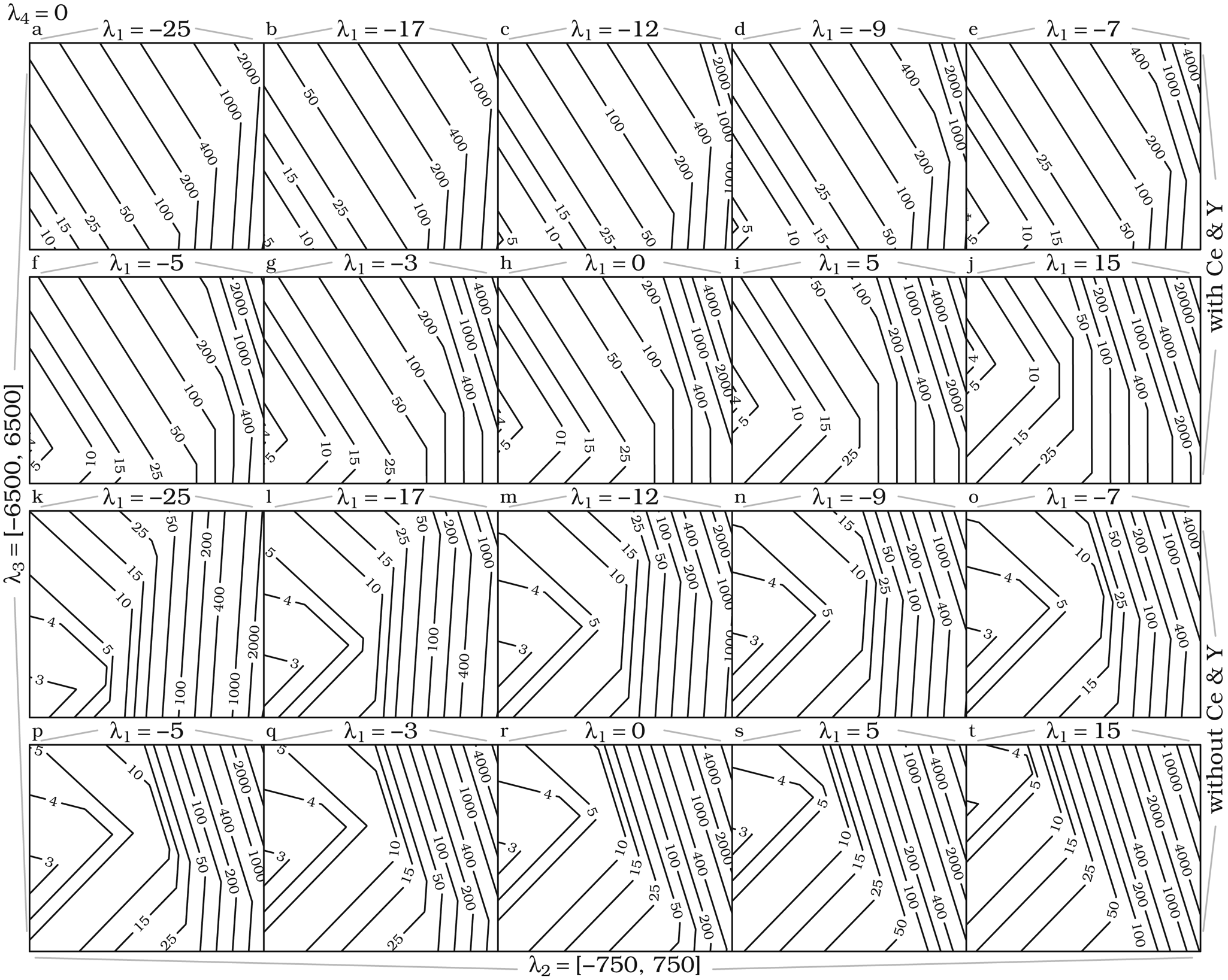
The anomalous redox behaviour of Eu allows its concentration in Ca-rich minerals, most notably plagioclase and epidote (Anenburg et al., Reference Anenburg, Katzir, Rhede, Jöns and Bach2015; Bédard, Reference Bédard2006; Bieseler et al., Reference Bieseler, Diehl, Jöns, Lucassen and Bach2018; Frei et al., Reference Frei, Liebscher, Franz, Dulski, Liebscher and Franz2004; Rudnick, Reference Rudnick1992; Schoneveld and O'Neill, Reference Schoneveld and O'Neill2019). It is possible to calculate the stage at which Eu becomes the most abundant REE in a mineral by calculating the ratio between the most abundant REE and Eu. The result is the minimum positive Eu anomaly required for it to predominate. Generally, Eu anomalies are calculated using the geometric mean of the neighbouring elements by Eu/Eu* =  ${\rm Eu/}\sqrt {{\rm Sm} \times {\rm Gd}} $, however this can lead to errors in patterns with strong curvature at Eu (see Fig. 5). Here, Eu anomalies are calculated relative to the expected Eu from the polynomial fit.

Fig. 5. A Nd–Tb portion of a pattern generated with λ0 = 1, λ1 = 0, λ2 = –300, and λ3 = –1000 and no Eu anomaly (green line). However, an attempt to calculate the anomaly using interpolation of the neighbouring elements (blue line) leads to  ${\rm Eu/Eu\ast } = {\rm Eu/}\sqrt {{\rm Sm} \times {\rm Gd}} = 1.05$, suggesting a small positive, yet spurious, Eu anomaly.
Figure 6 shows the Eu anomaly required for it to predominate at different λ values. As above, the removal of Ce and Y allows for smaller Eu anomalies to suffice. The greatest influence comes from λ2, which reduces the required anomaly as it becomes more negative. This is expected as patterns with negative λ2 are parabolic with maxima precisely at Eu. The required Eu anomalies close to the plot centres are often in the range of 5 to 10, which is a reasonable value often seen in nature. Prolonged surface weathering often leads to concentration of REE, and it is probable that Eu-dominated minerals will form in strongly weathered anorthosites or epidosites (e.g. Banerjee and Chakrabarti, Reference Banerjee and Chakrabarti2018).

Fig. 6. Contour maps showing the positive Eu anomaly relative to Eu expected from the polynomial required for Eu to be the most abundant REE. Construction of panels is similar to Fig. 3.
Comparison with natural minerals
Rare earth element patterns and polynomial fits calculated from data available for four Yb minerals and two Sm minerals are given in Fig. 7. The polynomial fits to the Yb minerals reasonably agree with the observed patterns. Likewise, projection of their coefficients into λ2 – λ3 space shows they all plot within their respective Yb fields (marked by similarly coloured lines). In contrast, the polynomial fits to the Sm minerals fail to reproduce the high Sm contents. Moreover, their projections plot outside of the Sm-dominant fields in λ2 – λ3 space. This could result from analytical challenges as the REE are measured by wavelength-dispersive spectroscopy, a method which suffers from peak overlaps and requires careful calibration and matrix corrections. Analytical problems aside, this could indicate an additional geochemical fractionation process not captured by the shape coefficient model. Such processes are common in low-temperature environments, some examples being the seemingly hydrothermal texture shown by the florencite-(Sm) domains described by Repina et al. (Reference Repina, Khiller and Makagonov2014). This method does not capture variability caused by the tetrad effect, which may become important at similar low temperatures or unusual fluid chemistries (Irber, Reference Irber1999; Monecke et al., Reference Monecke, Kempe, Monecke, Sala and Wolf2002).

Fig. 7. (a) Literature data for REE minerals and their corresponding polynomial fits. The macro provided by O'Neill (Reference O'Neill2016) requires data for Ce or La, which was not available for all minerals. See Supplementary material for resulting λ values, information on assumed values, and discarded values of poor data quality. (b) Projection of λ values used to construct the patterns in (a) to λ2–λ3 space. Coloured lines indicate the field boundaries for dominant Sm (red and blue) and Yb (all others). Data sources: Masau et al. (Reference Masau, Černý, Cooper, Chapman and Grice2002), Repina et al. (Reference Repina, Popova, Churin, Belogub and Khiller2011), Voloshin et al. (Reference Voloshin, Pakhomovskii, Men'shikov, Povarennykh, Matvinenko and Yakubovich1984), Voloshin et al. (Reference Voloshin, Pakhomovsky and Tyusheva1983), Simmons et al. (Reference Simmons, Hanson and Falster2006) and Buck et al. (Reference Buck, Cooper, Černý, Grice and Hawthorne1999).
Mineral evolution and nomenclature
There are fewer minerals with essential REE than expected according to their crustal abundance (Christy, Reference Christy2015; Hazen et al., Reference Hazen, Grew, Downs, Golden and Hystad2015a; Higgins and Smith, Reference Higgins and Smith2010; Krivovichev et al., Reference Krivovichev, Charykova and Krivovichev2018; Rieder, Reference Rieder2016). The Ca ionic radius is close to that of Pr (112 pm and 112.6 pm, respectively, Shannon, Reference Shannon1976), and consequently the LREE are often dispersed as trace elements in Ca-rich minerals. Minerals with smaller Ca sites (such as clinopyroxenes) or with rigid structures will strongly partition HREE relative to LREE (most notably garnet and zircon, Dubacq and Plunder, Reference Dubacq and Plunder2018) provided that charge balance is achieved. As a result, REE rarely form minerals of their own and instead occur as trace elements in other minerals. Even when REE do form their own minerals, they are dominated mostly by Ce and Y, with the less abundant REE incorporated as subordinate components in solid solution (i.e. they ‘mimic’ Ce and Y, Hazen et al., Reference Hazen, Hystad, Downs, Golden, Pires and Grew2015b). No single mineral is capable of isolating a single trivalent REE, but instead incorporate the entire REE series to various degrees. Nonetheless, some minerals have crystal chemical constraints that lead to preferential uptake of a narrower REE range, leading to exceptional concentration of a certain subset relative to the others (Mitchell et al., Reference Mitchell, Novgorodova, Semenov and Marfunin1994). Guidelines published by the International Mineralogical Association Commission on New Minerals, Nomenclature and Classification (IMA–CNMNC) require names of minerals containing essential REE to have a suffix denoting the most abundant REE (Hatert et al., Reference Hatert, Mills, Pasero and Williams2013; Nickel and Grice, Reference Nickel and Grice1998). These suffixes are known as ‘Levinson’ suffixes (Bayliss and Levinson, Reference Bayliss and Levinson1988; Levinson, Reference Levinson1966). Insofar as nomenclature is inevitably subjective, it could be hard to justify naming a new mineral species. For example, instances of florencite-(Sm) described by Repina et al. (Reference Repina, Popova, Churin, Belogub and Khiller2011) are not individual grains, but rather Sm-dominated thin growth zones inside florencite-(Ce). Hazen (Reference Hazen2019) argued that the diversity of REE minerals is an artificial construct by the IMA–CNMNC mineral names rules. He states: “…these split species represent a single natural kind with one stability field that incorporates yttrium and a range of light and heavy REE and thus one paragenetic mode” (Hazen, Reference Hazen2019). However, this statement misses a great deal of nuance in REE geochemistry. Indeed, two minerals with similar REE contents but one containing La/Ce = 0.95 and the other La/Ce = 1.05 will share similar thermodynamic properties and virtually indistinguishable stability fields, even though they will have different mineral names. This is not the case for elements that are farther apart. For example, the thermodynamic properties of bastnäsite-(Ce) and bastnäsite-(Y), or hingganite-(Ce) and hingganite-(Yb) are probably sufficiently different to justify their own mineral species (e.g. Miyawaki and Nakai, Reference Miyawaki, Nakai, Jones, Wall and Williams1996)—probably more than zircon and hafnon are justified.
The rarity of REE minerals dominated by Sm, Gd, Dy, Er or Yb is a direct consequence of the composition (X) component of the Hazen and Ausubel (Reference Hazen and Ausubel2016) first criterion for mineral rarity: P–T–X range. As shown above, the formation of most Y-absent HREE-dominated species require a negative Y anomaly, and a negative Ce anomaly allows greater dominance of La and Nd. These anomalies require distinct geochemical conditions, either F-rich fluids (Loges et al., Reference Loges, Migdisov, Wagner, Williams-Jones and Markl2013) or coexistence of fluorite for Y anomalies (Chebotarev et al., Reference Chebotarev, Veksler, Wohlgemuth-Ueberwasser, Doroshkevich and Koch-Müller2019), and oxidising conditions coupled with low temperatures for Ce anomalies (Anenburg et al., Reference Anenburg, Burnham and Mavrogenes2018; Burnham and Berry, Reference Burnham and Berry2014; Sørensen, Reference Sørensen1976). The small Sm-dominant zones inside florencite grains reported by Repina et al. (Reference Repina, Popova, Churin, Belogub and Khiller2011) require exceptional formation conditions (Repina et al., Reference Repina, Khiller and Makagonov2014). Therefore, ‘one paragenetic mode’ cannot account for the entire diversity observed in REE mineral name suffixes, and they do not represent ‘a single natural kind’ (also remembering that the ‘natural kind’ concept and mineralogy are incompatible; Santana, Reference Santana2019). The processes that lead to one REE predominating over another are real fractionation processes occurring in Nature. It follows that identification of REE minerals with uncommon dominant elements expand our recognition of attainable extremes in terrestrial geochemical fractionation processes (Hazen and Ausubel, Reference Hazen and Ausubel2016).
The predominant REE in a mineral is not an arbitrary element that gained dominance by happenstance. As seen in Figs 3 and 4, each element dominates a specific region in λ-space. An arbitrary linear-like path in n-dimensional λn space will systematically cross different elements, each with its own characteristic range of REE patterns. Therefore, the Levinson suffix for a mineral is a good indication for its REE pattern type and range of possible λ shape coefficients, which may provide information about the process that led to the mineral forming (e.g. by the use of ψ polynomials which represent mineral/melt partition coefficients; O'Neill, Reference O'Neill2016).
Notwithstanding the merit of Levinson suffixes in providing information on likely mineral REE patterns and fractionation processes, it has limitations. For example, a ‘-(La)’ suffix does not reveal whether La dominance results from a negative Ce anomaly or from exceptionally high λ1 and λ2. Furthermore, the inclusion of Y in the suffixes obscures much of the variability in the HREE. There is only one Gd mineral and four Yb minerals in which Y contents are low enough to allow a lanthanide to predominate. However, when excluding Y, a much greater diversity is revealed, such as Dy-rich chernovite-(Y) (Ondrejka et al., Reference Ondrejka, Uher, Pršek and Ozdín2007), Yb-rich chernovite-(Y) (Alekseev and Marin, Reference Alekseev and Marin2014) and Gd-rich gagarinite-(Y) (Savelyeva et al., Reference Savelyeva, Bazarova, Khromova and Kanakin2019). A more thorough literature review will undoubtedly reveal more Gd-, Dy-, and Yb-dominant species, and potentially Er-dominant species, when disregarding Y. The grouping of lanthanides and Y together as the REE is reasonable when discussing high-temperature or large-scale processes. Nonetheless, the behaviour of Y is not identical to the lanthanides (Bédard, Reference Bédard2014; Schoneveld and O'Neill, Reference Schoneveld and O'Neill2019). For example, in the context of the tetrad effect, the Y/Ho ratio progressively differs from the chondritic in step with the magnitude of the tetrad effect (e.g. Irber, Reference Irber1999). This difference becomes pronounced on small scales such as those of a mineral grain, leading to strong decoupling of Y and the lanthanides, and Y no longer forms a coherent part of the REE (e.g. Anenburg et al., Reference Anenburg, Mavrogenes and Bennett2020b).
The geochemical behaviour of the REE as part of a series and the resulting dilution of each element by others (Christy, Reference Christy2015; Mitchell et al., Reference Mitchell, Novgorodova, Semenov and Marfunin1994) may not be the only reason for the apparent lack of HREE minerals. The low HREE mineral diversity is probably an artefact of the inclusion of Y as the Levinson suffix in mineral names. Hazen et al. (Reference Hazen, Hummer, Hystad, Downs and Golden2016), for instance, predicts many more REE-carbonates are yet to be found. This study demonstrates that once HREE mineral chemistry is looked at beyond Y, a greater diversity is discovered. It is possible that many more REE minerals—which reflect real geochemical fractionation processes—will be ‘rediscovered’ if Y is removed from Levinson suffixes. Furthermore, future advances in analytical methods are likely to reveal small scale heterogeneities in which unusual REE will predominate (Cook et al., Reference Cook, Ciobanu, Ehrig, Slattery, Verdugo-Ihl, Courtney-Davies and Gao2017).
Supplementary material
To view supplementary material for this article, please visit https://doi.org/10.1180/mgm.2020.70
Acknowledgements
Hugh O'Neill is thanked for thought-provoking discussions. Stuart Mills is thanked for his editorial handling.
Data
All data and figures in this article were generated using R 4.0.2 from the R script ‘REEpatterns.R’ available in the Supplementary materials.
Appendix
ALambdaR is an online interactive app developed in R that generates REE patterns from input describing the REE pattern shape, available at https://lambdar.rses.anu.edu.au/alambdar/. The app takes numerical input of λ0 to λ4, Eu and Ce anomalies and Y/Ho ratio. It generates REE abundances from which it shows a normalised REE pattern according to a normalisation scheme selected by the user. A pie chart showing the relative properties of all REE is also given. It is possible to export the plots in either pdf (vector) or png (raster) formats, and export the data in comma separated values (csv) format. The app also allows upload of files in csv format containing multiple combinations of λ0 to λ4, and it generates a downloadable file containing the resulting REE abundances in μg g–1 units. Future versions will include tetrad effects for a more comprehensive REE pattern generation functionality (e.g. Irber, Reference Irber1999; Minami and Masuda, Reference Minami and Masuda1997; Monecke et al., Reference Monecke, Kempe, Monecke, Sala and Wolf2002).
For calculating a REE pattern using λ shape coefficients, the app uses a matrix F that includes all fn values:
 $${\bi F} = \left({\matrix{ {{\rm f}_{{\rm La\comma 1}}} & \cdots & {{\rm f}_{{\rm La\comma 4}}} \cr {{\rm f}_{{\rm Ce\comma 1}}} & \cdots & {{\rm f}_{{\rm Ce\comma 4}}} \cr \vdots & \ddots & \vdots \cr {{\rm f}_{{\rm Lu\comma 1}}} & \cdots & {{\rm f}_{{\rm Lu\comma 4}}} \cr } } \right) = \left({\hskip5pt \matrix{ {0.1052} & \cdots & {8.29 \times {10}^{{-}6}} \cr {0.0882} & \cdots & \hskip-6.9pt {-7.16 \times {10}^{{-}6}} \cr \vdots & \ddots & \vdots \cr {\hskip-7pt -0.0778} & \cdots & {9.41 \times {10}^{{-}6}} \cr } } \right)$$
The full set of values is available in O'Neill (Reference O'Neill2016) or in the Supplementary code. Each REE pattern can be described as a combination of λ values, and a column vector is defined:
 $$\vec{\lambda } = \left({\matrix{ {{\rm \lambda }_1} \cr {{\rm \lambda }_2} \cr {{\rm \lambda }_3} \cr {{\rm \lambda }_4} \cr } } \right)$$
The REE contents for each corresponding  $\vec{{\rm \lambda }}$ can be calculated using matrix multiplication:
 $$\overrightarrow {\ln \left({\displaystyle{{\lsqb {{\rm REE}} \rsqb } \over {{\lsqb {{\rm REE}} \rsqb }_{{\rm CI}}}}} \right)} = {\bi \;F}\vec{\lambda } + {\rm \lambda }_0.$$
The choice of the logarithm base does not change the pattern shape. However, in some cases it might be desirable to transform the values to base 10 which is achieved via:
 $$\overrightarrow {\log \left({\displaystyle{{\lsqb {{\rm REE}} \rsqb } \over {{\lsqb {{\rm REE}} \rsqb }_{{\rm CI}}}}} \right)} = \log e \times \overrightarrow {\ln \left({\displaystyle{{\lsqb {{\rm REE}} \rsqb } \over {{\lsqb {{\rm REE}} \rsqb }_{{\rm CI}}}}} \right)} $$
If required, concentration values in μg g–1 are calculated using:
 $$\overrightarrow {\lsqb {{\rm REE}} \rsqb } = \vec{C}\cdot e^{\overrightarrow {\ln \left({{{\lsqb {{\rm REE}} \rsqb } \over {{\lsqb {{\rm REE}} \rsqb }_{{\rm CI}}}}} \right)} } = \vec{C}\cdot 10^{\overrightarrow {\log \left({{{\lsqb {{\rm REE}} \rsqb } \over {{\lsqb {{\rm REE}} \rsqb }_{{\rm CI}}}}} \right)} }$$
Where  $\vec{C}$ is a vector of CI values from O'Neill (Reference O'Neill2016).