


1 Introduction
Integrating multiple fluidic processes into a single platform has become progressively important in modern lab-on-a-chip devices where separation and mixing often turn out to be two of the most critical processes (Hunter Reference Hunter1981; Probstein Reference Probstein1994; Stroock et al. Reference Stroock, Dertinger, Ajdari, Mezic, Stone and Whitesides2002; Ghosal Reference Ghosal2004; Stone, Stroock & Ajdari Reference Stone, Stroock and Ajdari2004; Masliyah & Bhattacherjee Reference Masliyah and Bhattacherjee2006; Whitesides Reference Whitesides2006). With the rapid advancement in microfabrication technologies, a large number of research efforts have been dedicated towards developing strategies for improved fluidic mixing or separation (Anderson et al. Reference Anderson, Galaktionov, Peters, Van De Vosse and Meijer2000; Glasgow, Batton & Aubry Reference Glasgow, Batton and Aubry2004; Karniadakis, Beskok & Aluru Reference Karniadakis, Beskok and Aluru2005; Zhang, He & Liu Reference Zhang, He and Liu2006; Chang & Yang Reference Chang and Yang2008; Sugioka Reference Sugioka2010; Ghosh & Chakraborty Reference Ghosh and Chakraborty2012). Towards achieving enhanced mixing in microdevices, diffusion and dispersion are undoubtedly the two most common phenomena. Accordingly, significant research interest in this domain has developed over the past years, with a vision of employing different flow-actuating mechanisms as well as geometric alterations in the fluidic pathways, so as to achieve the desired functionalities.
Although flow actuation using electric fields has wide spectrum of applications in both engineering and medical domains (Becker & Gärtner Reference Becker and Gärtner2000; Garcia et al. Reference Garcia, Ista, Petsev and López2005; Van Der Heyden, Stein & Dekker Reference Van Der Heyden, Stein and Dekker2005; Das, Das & Chakraborty Reference Das, Das and Chakraborty2006; Das & Chakraborty Reference Das and Chakraborty2007; Haeberle & Zengerle Reference Haeberle and Zengerle2007; Ohno, Tachikawa & Manz Reference Ohno, Tachikawa and Manz2008; Berli Reference Berli2010; Mark et al. Reference Mark, Haeberle, Roth, Von Stetten and Zengerle2010; Zhao Reference Zhao2011; Bandopadhyay & Chakraborty Reference Bandopadhyay and Chakraborty2012; Nguyen et al. Reference Nguyen, Xie, De Vreede, Van Den Berg and Eijkel2013; Goswami et al. Reference Goswami, Chakraborty, Bandopadhyay and Chakraborty2015; Das et al. Reference Das, Kar, Anwar, Saha and Chakraborty2018), one of the major aspects of the classical electro-osmotic flow in the presence of homogeneous interfacial conditions is the existence of the uniform velocity profile which arises when the electrical double layer (EDL) becomes very thin compared to the channel dimension (Ghosal Reference Ghosal2004; Masliyah & Bhattacherjee Reference Masliyah and Bhattacherjee2006). This results in a plug-type velocity distribution, thus reducing the extent of mixing significantly.
Hydrodynamic dispersion is the band broadening of a solute which mainly arises from the non-uniformity in the flow field (Taylor Reference Taylor1953; Aris Reference Aris1956, Reference Aris1959; Chatwin Reference Chatwin1970, Reference Chatwin1975; Chatwin & Sullivan Reference Chatwin and Sullivan1982; Smith Reference Smith1982; Barton Reference Barton1983; Watson Reference Watson1983; Mazumder & Das Reference Mazumder and Das1992; Ng & Yip Reference Ng and Yip2001; Zholkovskij & Masliyah Reference Zholkovskij and Masliyah2004; Ajdari, Bontoux & Stone Reference Ajdari, Bontoux and Stone2006; Ng Reference Ng2006; Ghosal Reference Ghosal2006; Jansons Reference Jansons2006; Sounart & Baygents Reference Sounart and Baygents2007; Dutta Reference Dutta2008; Datta & Ghosal Reference Datta and Ghosal2008; Ghosal & Chen Reference Ghosal and Chen2012; Arcos et al. Reference Arcos, Méndez, Bautista and Bautista2018; Chu et al. Reference Chu, Garoff, Przybycien, Tilton and Khair2019). Under ideal circumstances, the velocity profile of electro-osmotic flow does not contribute to shear-induced axial dispersion because of the flatness of the velocity profile as opposed to the case of Poiseuille flow (which is parabolic in nature) (Gaš, Štědrý & Kenndler Reference Gaš, Štědrý and Kenndler1997; Ghosal Reference Ghosal2004; Mukherjee et al. Reference Mukherjee, Dhar, Dasgupta and Chakraborty2019). However, in practice, any inhomogeneity in the flow condition or flow domain can give rise to strong perturbation in the flow field, thereby inducing an axial pressure gradient, which is accompanied by the generation of secondary flow component in order to maintain the flow continuity. In applications demanding augmented dispersion, classical electro-osmotic flow is modulated in two ways, either bringing non-uniformity in the channel geometry or introducing axial variation in the zeta potential (Ajdari Reference Ajdari1995, Reference Ajdari1996; Ghosal Reference Ghosal2002; Mandal et al. Reference Mandal, Ghosh, Bandopadhyay and Chakraborty2015; Ghosh, Mandal & Chakraborty Reference Ghosh, Mandal and Chakraborty2017; Arcos et al. Reference Arcos, Méndez, Bautista and Bautista2018).
Over the years, conventional studies of electrokinetics mainly directed their focus towards different techniques of flow actuation, energy conversion and zeta potential measurement under isothermal flow conditions (Levine et al. Reference Levine, Marriott, Neale and Epstein1975; Zeng et al. Reference Zeng, Chen, Mikkelsen and Santiago2001; Sinton et al. Reference Sinton, Escobedo-Canseco, Ren and Li2002; Brask, Kutter & Bruus Reference Brask, Kutter and Bruus2005; Gao et al. Reference Gao, Wong, Yang and Ooi2005; Venditti, Xuan & Li Reference Venditti, Xuan and Li2006; Li, Wong & Nguyen Reference Li, Wong and Nguyen2009; Mogensen et al. Reference Mogensen, Gangloff, Boggild, Teo, Milne and Kutter2009; Das & Chakraborty Reference Das and Chakraborty2010; Bandopadhyay & Chakraborty Reference Bandopadhyay and Chakraborty2011; Li, Wong & Nguyen Reference Li, Wong and Nguyen2011). The corresponding literature for non-isothermal flow is relatively scarce because of the lack of understanding of the physics involved. In non-isothermal systems, several complexities come into the picture. First, the modulated thermo-physical properties of an electrolyte solution, like viscosity, electrical permittivity, thermal conductivity, ionic diffusivity and thermophoretic mobility, in the presence of a thermal gradient, strongly influence the fluid motion. Besides this alteration in hydrodynamics, an additional contribution of dielectrophoretic body force due to permittivity variation, accompanied by an induced axial pressure gradient, comes into play in addition to the conventional electrokinetic forcing, thereby bringing complexity to the flow physics (Ghonge et al. Reference Ghonge, Chakraborty, Dey and Chakraborty2013; Dietzel & Hardt Reference Dietzel and Hardt2017). Additionally, zeta potential, which plays a crucial dole in governing the flow physics in electrokinetic flows, no longer remains constant in the presence of a thermal gradient (Revil et al. Reference Revil, Schwaeger, Cathles and Manhardt1999; Reppert Reference Reppert2003; Revil, Pezard & Glover Reference Revil, Pezard and Glover2003; Venditti et al. Reference Venditti, Xuan and Li2006; Ghonge et al. Reference Ghonge, Chakraborty, Dey and Chakraborty2013). Also, the determination of the temperature field may require a knowledge of other effects like heat generation due to induced streaming field or viscous dissipation which in turn affect fluid physical properties and convective contribution to the temperature distribution. Apart from this, contrary to the conventional electrokinetic studies, the assumption of mechanical equilibrium of ions within the electrical double layer (under isothermal conditions) is no longer valid where the effect of thermo-diffusion of ions needs to be incorporated in the transport equation of ionic species along with other components (Zhou et al. Reference Zhou, Xie, Yang and Cheong Lam2015; Zhang et al. Reference Zhang, Wang, Zeng and Zhao2019).
The distortion of the local equilibrium of ions in the electrical double layer (EDL) creates a departure from the classical Boltzmann distribution of ions which has direct consequences for the potential distribution. This alteration in charge distribution influences the flow dynamics via electrokinetic forcing, where the intricate coupling between thermal and electrical effects is already prevalent through the aforesaid property variation and an additional dielectrophoretic force. Further, in the absence of any external electric field, the net ionic current turns out to be zero. This condition is itself another source of nonlinearity in the analysis where both conduction and streaming current undergo marked alteration under the influence of finite temperature difference. In addition, it is worth mentioning that, when an electrolyte solution is subjected to an imposed temperature gradient, a thermoelectric field is induced by virtue of the movement of ions in response to the thermal driving force, commonly known as the Soret effect (Ghonge et al. Reference Ghonge, Chakraborty, Dey and Chakraborty2013; Zhou et al. Reference Zhou, Xie, Yang and Cheong Lam2015; Dietzel & Hardt Reference Dietzel and Hardt2016, Reference Dietzel and Hardt2017; Zhang et al. Reference Zhang, Wang, Zeng and Zhao2019). Moreover, an additional form of thermoelectric field can be induced within the system because of the diffusivity difference between the ions even if their Soret coefficients remain the same. Besides, the mode of application of thermal gradient can cause significant rearrangement of ions within the EDL and, hence, the subsequent potential distribution for a transverse temperature gradient may not necessarily be the same as that for longitudinal temperature gradient, altering the hydrodynamics in a rather profound manner. Considering the aforementioned intricacies in coupling thermal, electrical and hydrodynamical effects in micro-confinements, research efforts towards addressing various aspects of thermo-solutal convection of electrolyte solutions have turned out to be relatively inadequate, despite having widespread applications in processes like water treatment, charge separation, zeta potential determination, waste heat recovery and energy conversion (Würger Reference Würger2008, Reference Würger2010; Sandbakk, Bentien & Kjelstrup Reference Sandbakk, Bentien and Kjelstrup2013; Dietzel & Hardt Reference Dietzel and Hardt2016; Jokinen et al. Reference Jokinen, Manzanares, Kontturi and Murtomäki2016; Barragán & Kjelstrup Reference Barragán and Kjelstrup2017; Dietzel & Hardt Reference Dietzel and Hardt2017; Li & Wang Reference Li and Wang2018). As such, the research focus in this domain has been directed primarily towards incorporating non-isothermal effects as a secondary force in the alteration of hydrodynamics of simple fluids (Maynes & Webb Reference Maynes and Webb2003; Tang et al. Reference Tang, Yang, Chai and Gong2003; Xuan et al. Reference Xuan, Xu, Sinton and Li2004; Chakraborty Reference Chakraborty2006; Huang & Yang Reference Huang and Yang2006; Xuan Reference Xuan2008; Garai & Chakraborty Reference Garai and Chakraborty2009; Sadeghi et al. Reference Sadeghi, Yavari, Saidi and Chakraborty2011; Dey, Chakraborty & Chakraborty Reference Dey, Chakraborty and Chakraborty2011; Sánchez et al. Reference Sánchez, Ascanio, Méndez and Bautista2018). Therefore, except for some limited physical scenarios, such an exclusive effect has not been utilized to a significant practical benefit (Dietzel & Hardt Reference Dietzel and Hardt2016, Reference Dietzel and Hardt2017; Zhang et al. Reference Zhang, Wang, Zeng and Zhao2019).
Recently, incorporation of a thermal gradient has emerged as an alternative tool in augmenting dispersion where interplay between thermal and electrical effects over small length scales, almost exclusively, dictates the flow physics (Chen et al. Reference Chen, Lin, Lele and Santiago2005; Sánchez et al. Reference Sánchez, Ascanio, Méndez and Bautista2018; Mukherjee et al. Reference Mukherjee, Dhar, Dasgupta and Chakraborty2019). In addition, it may be noted that with the emergence of new-generation medical devices, complex bio-fluids have more prominently come into the paradigm of microfluidics (Das & Chakraborty Reference Das and Chakraborty2006; Berli & Olivares Reference Berli and Olivares2008; Olivares, Vera-Candioti & Berli Reference Olivares, Vera-Candioti and Berli2009; Berli Reference Berli2010; Zhao & Yang Reference Zhao and Yang2011, Reference Zhao and Yang2013). Such fluids exhibit strikingly distinct behaviour compared to the fluids obeying Newton’s law of viscosity (Owens Reference Owens2006; Fam, Bryant & Kontopoulou Reference Fam, Bryant and Kontopoulou2007; Moyers-Gonzalez, Owens & Fang Reference Moyers-Gonzalez, Owens and Fang2008; De Loubens et al. Reference De Loubens, Magnin, Doyennette, Tréléa and Souchon2011; Brust et al. Reference Brust, Schaefer, Doerr and Wagner2013; Silva, Alves & Oliveira Reference Silva, Alves and Oliveira2017). Some recent studies have demonstrated that the constitutive behaviour of these biological fluids has close resemblance to the rheology of viscoelastic fluids, and therefore the inclusion of fluid rheology and viscoelasticity in dispersion characteristics has attracted significant attention lately (Brust et al. Reference Brust, Schaefer, Doerr and Wagner2013; Arcos et al. Reference Arcos, Méndez, Bautista and Bautista2018; Hoshyargar et al. Reference Hoshyargar, Talebi, Ashrafizadeh and Sadeghi2018; Mukherjee et al. Reference Mukherjee, Dhar, Dasgupta and Chakraborty2019). While considering the thermally induced electrokinetic flow of viscoelastic fluids, an additional source of nonlinearity crops up as mediated by the constitutive behaviour of the fluid (Afonso, Alves & Pinho Reference Afonso, Alves and Pinho2009; Coelho, Alves & Pinho Reference Coelho, Alves and Pinho2012; Afonso, Alves & Pinho Reference Afonso, Alves and Pinho2013; Ghosh & Chakraborty Reference Ghosh and Chakraborty2015; Ferrás et al. Reference Ferrás, Afonso, Alves, Nóbrega and Pinho2016; Ghosh, Chaudhury & Chakraborty Reference Ghosh, Chaudhury and Chakraborty2016; Mukherjee et al. Reference Mukherjee, Das, Dhar, Chakraborty and Dasgupta2017a ,Reference Mukherjee, Goswami, Dhar, Dasgupta and Chakraborty b ). Moreover, the degree of viscoelasticity, which is determined using physical properties like fluid viscosity and relaxation time, is a strong function of the prevalent thermal gradient, augmenting the complexity of the problem to a large extent (Bautista et al. Reference Bautista, Sánchez, Arcos and Méndez2013; Mukherjee et al. Reference Mukherjee, Dhar, Dasgupta and Chakraborty2019).
To the best of our knowledge, dispersion characteristics of thermally induced electrokinetic transport of complex fluids in microfluidic environments, where the temperature gradient is solely used for flow manipulation, have not been addressed in the literature. Here, we report the effect of an external temperature gradient on the dispersion characteristics of an electrolyte solution in a parallel-plate microchannel. We subsequently discuss the charge redistribution upon application of the thermal gradient, subsequent perturbation of the fluid motion and its implications for hydrodynamic dispersion, considering both Newtonian and viscoelastic fluids. Our results reveal that by combining some of the electrokinetic, thermal and fluidic parameters coupled with rheological aspects, it is possible to achieve massively augmented solute dispersion, while for some combinations significant enhancement in streaming potential (compared to the solely pressure-driven flow) can also be obtained. We believe that the present analysis can be used as a fundamental basis in the design of thermally actuated micro- and bio-fluidic devices demanding improved solute dispersion where the interplay between electromechanics, thermal effects, hydrodynamics and rheological aspects in narrow confinement can be coupled together to a beneficial effect. Additionally, a wide variety of thermal and fluidic problems can also be approached on the basis of the present theoretical framework (Raj et al. Reference Raj, Sarkar, Chakraborty, Phanikumar, Dutta and Chattopadhyay2002; Das, Chakraborty & Dutta Reference Das, Chakraborty and Dutta2004; Chakraborty & Chakraborty Reference Chakraborty and Chakraborty2007; Ghatak & Chakraborty Reference Ghatak and Chakraborty2007; Chakraborty & Srivastava Reference Chakraborty and Srivastava2007; Chakraborty & Padhy Reference Chakraborty and Padhy2008).

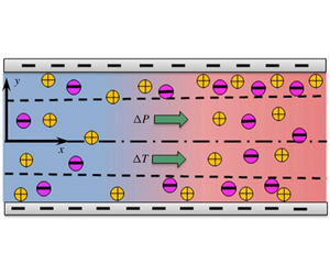
Figure 1. Schematic of the combined pressure-driven and temperature-gradient-induced flow of electrolyte solution through a parallel-plate microchannel. (a) Temperature gradient is applied in the axial direction. (b) Temperature gradient is applied in the transverse direction.
2 Problem formulation
We consider non-isothermal electrokinetic flow of a binary $1:1$
symmetric electrolyte solution through a parallel-plate microchannel. We choose a rectangular Cartesian coordinate system where
$1:1$
symmetric electrolyte solution through a parallel-plate microchannel. We choose a rectangular Cartesian coordinate system where $x$
and
$x$
and $y$
coordinates represent longitudinal and transverse directions, respectively, while the origin is placed at the centreline of the channel. Length scales in the two directions are
$y$
coordinates represent longitudinal and transverse directions, respectively, while the origin is placed at the centreline of the channel. Length scales in the two directions are $l$
and
$l$
and $h$
, respectively, where the half-channel height (
$h$
, respectively, where the half-channel height ( $h$
) is very small compared to the channel length (
$h$
) is very small compared to the channel length ( $l$
), i.e.
$l$
), i.e. $h\ll l$
or
$h\ll l$
or $\unicode[STIX]{x1D6FD}=h/l\ll 1$
. We have employed two different types of thermal gradients: case 1, axially applied temperature gradient; case 2, temperature gradient applied in the transverse direction (figure 1).
$\unicode[STIX]{x1D6FD}=h/l\ll 1$
. We have employed two different types of thermal gradients: case 1, axially applied temperature gradient; case 2, temperature gradient applied in the transverse direction (figure 1).
2.1 Dispersion coefficient: a broad perspective
We consider the hydrodynamic dispersion characteristics of a combined pressure-driven and thermal-gradient-driven electrokinetic flow of an electrolyte solution. According to the definition of the band-broadening phenomenon, the hydrodynamic dispersion coefficient $(\overline{D}_{eff})$
depends on the rate of change of variance of solute displacement band as
$(\overline{D}_{eff})$
depends on the rate of change of variance of solute displacement band as $D_{eff}=\frac{1}{2}(\text{d}/\text{d}t)\unicode[STIX]{x1D70E}^{2}(t)$
, where
$D_{eff}=\frac{1}{2}(\text{d}/\text{d}t)\unicode[STIX]{x1D70E}^{2}(t)$
, where $\unicode[STIX]{x1D70E}^{2}$
is the variance of solute displacement. This temporal variation with respect to the centroid of the band depends on the plate height (
$\unicode[STIX]{x1D70E}^{2}$
is the variance of solute displacement. This temporal variation with respect to the centroid of the band depends on the plate height ( $h^{\prime }$
) as
$h^{\prime }$
) as $h^{\prime }=(\text{d}/\text{d}x^{\prime })\unicode[STIX]{x1D70E}^{2}(x^{\prime })$
, where
$h^{\prime }=(\text{d}/\text{d}x^{\prime })\unicode[STIX]{x1D70E}^{2}(x^{\prime })$
, where $x^{\prime }$
denotes the location of the band centroid. Knowledge of the plate height is necessary in determining the dispersion coefficient because of its ability to incorporate any change in the variance of the mean concentration. For a band of non-adsorbing solute flowing in a rectangular channel, the velocity of the centre mass becomes equal to the mean axial velocity of flow, i.e.
$x^{\prime }$
denotes the location of the band centroid. Knowledge of the plate height is necessary in determining the dispersion coefficient because of its ability to incorporate any change in the variance of the mean concentration. For a band of non-adsorbing solute flowing in a rectangular channel, the velocity of the centre mass becomes equal to the mean axial velocity of flow, i.e. $u_{avg}=\text{d}x^{\prime }/\text{d}t$
. Using the descriptions of
$u_{avg}=\text{d}x^{\prime }/\text{d}t$
. Using the descriptions of $h^{\prime }$
and
$h^{\prime }$
and $x^{\prime }$
, one can rewrite the expression of the dispersion coefficient as
$x^{\prime }$
, one can rewrite the expression of the dispersion coefficient as
 $$\begin{eqnarray}\displaystyle D_{eff}=u_{avg}h^{\prime }/2. & & \displaystyle\end{eqnarray}$$
Here, $u_{avg}$
is the mean velocity averaged cross-sectionally. As reported in the literature (Van Deemter, Zuiderweg & Klinkenberg Reference Van Deemter, Zuiderweg and Klinkenberg1956), the plate height is related to the mean velocity as
$u_{avg}$
is the mean velocity averaged cross-sectionally. As reported in the literature (Van Deemter, Zuiderweg & Klinkenberg Reference Van Deemter, Zuiderweg and Klinkenberg1956), the plate height is related to the mean velocity as
 $$\begin{eqnarray}h^{\prime }=2D/u_{avg}+(u_{avg}h_{min}^{2}/8D).\end{eqnarray}$$
In (2.2), $h_{min}$
is the minimum plate height for a given flow condition and
$h_{min}$
is the minimum plate height for a given flow condition and $D$
is diffusivity. On the right-hand side, the contribution of the molecular diffusion is represented by the first term while the second term represents the contribution due to the non-uniformity in the flow field. By following some recent studies (Arcos et al.
Reference Arcos, Méndez, Bautista and Bautista2018; Hoshyargar et al.
Reference Hoshyargar, Talebi, Ashrafizadeh and Sadeghi2018), we have used the following expression for evaluating
$D$
is diffusivity. On the right-hand side, the contribution of the molecular diffusion is represented by the first term while the second term represents the contribution due to the non-uniformity in the flow field. By following some recent studies (Arcos et al.
Reference Arcos, Méndez, Bautista and Bautista2018; Hoshyargar et al.
Reference Hoshyargar, Talebi, Ashrafizadeh and Sadeghi2018), we have used the following expression for evaluating $h_{min}$
:
$h_{min}$
:
 $$\begin{eqnarray}h_{min}^{2}=\frac{16}{h}\int _{0}^{h}\int _{0}^{y}[\{(u/u_{avg})-1\}\,\text{d}y]^{2}\,\text{d}y.\end{eqnarray}$$
Combining all this, the dimensionless form of the dispersion coefficient $(\overline{D}_{eff})$
reads as
$(\overline{D}_{eff})$
reads as
 $$\begin{eqnarray}\overline{D}_{eff}=1+(Pe_{D}\overline{u}_{avg}\overline{h}_{min})^{2}/16,\end{eqnarray}$$
where $Pe_{D}$
is the dispersion Peclet number,
$Pe_{D}$
is the dispersion Peclet number, $\overline{h}_{min}=h_{min}/h$
and
$\overline{h}_{min}=h_{min}/h$
and $\overline{u}_{avg}=u_{avg}/u_{c}$
is the dimensionless average flow velocity with
$\overline{u}_{avg}=u_{avg}/u_{c}$
is the dimensionless average flow velocity with $u_{c}$
being the characteristic velocity scale.
$u_{c}$
being the characteristic velocity scale.
For the sake of brevity, the detailed mathematical expressions for obtaining the hydrodynamic dispersion coefficient are presented in § A of the supplementary material, available at https://doi.org/10.1017/jfm.2020.369, which clearly illustrates the complicated mathematical and physical interplay of the solutal, hydrodynamic and thermal fields, restrained by the consideration of overall electroneutrality. As clear from the definition, the dispersion coefficient depends directly on the velocity field, which in turn is influenced strongly by the charge distribution modulated by external temperature gradient, mediated by a two-way coupling. The governing equations delineating the same are discussed in the subsequent subsection.
2.2 Governing equations and boundary conditions
In this section, we first present the governing equation for the temperature distribution. Unlike conventional streaming-field-induced electrokinetic flow, here temperature ( $T$
) within the microchannel does not remain constant which is given by the following energy equation:
$T$
) within the microchannel does not remain constant which is given by the following energy equation:
 $$\begin{eqnarray}\unicode[STIX]{x1D70C}C_{p}\left(u\frac{\unicode[STIX]{x2202}T}{\unicode[STIX]{x2202}x}+v\frac{\unicode[STIX]{x2202}T}{\unicode[STIX]{x2202}y}\right)=\frac{\unicode[STIX]{x2202}}{\unicode[STIX]{x2202}x}\left(k\frac{\unicode[STIX]{x2202}T}{\unicode[STIX]{x2202}x}\right)+\frac{\unicode[STIX]{x2202}}{\unicode[STIX]{x2202}y}\left(k\frac{\unicode[STIX]{x2202}T}{\unicode[STIX]{x2202}y}\right)+Q_{gen}+Q_{vd},\end{eqnarray}$$
where the left-hand side is the advective contribution, the first two terms on the right-hand side are the conductive contributions, $Q_{gen}=\unicode[STIX]{x1D70E}E_{x}^{2}=(2z^{2}e^{2}Dn_{\infty }/k_{B}T)(-\unicode[STIX]{x2202}\unicode[STIX]{x1D719}/\unicode[STIX]{x2202}x)^{2}$
is the heat generation term due to the induced streaming field and
$Q_{gen}=\unicode[STIX]{x1D70E}E_{x}^{2}=(2z^{2}e^{2}Dn_{\infty }/k_{B}T)(-\unicode[STIX]{x2202}\unicode[STIX]{x1D719}/\unicode[STIX]{x2202}x)^{2}$
is the heat generation term due to the induced streaming field and $Q_{vd}=\unicode[STIX]{x1D707}[2\{(\unicode[STIX]{x2202}u/\unicode[STIX]{x2202}x)^{2}+(\unicode[STIX]{x2202}v/\unicode[STIX]{x2202}y)^{2}\}+(\unicode[STIX]{x2202}u/\unicode[STIX]{x2202}y+\unicode[STIX]{x2202}v/\unicode[STIX]{x2202}x)^{2}]-\frac{2}{3}\unicode[STIX]{x1D707}(\unicode[STIX]{x1D735}\boldsymbol{\cdot }v)^{2}$
is the viscous dissipation term with
$Q_{vd}=\unicode[STIX]{x1D707}[2\{(\unicode[STIX]{x2202}u/\unicode[STIX]{x2202}x)^{2}+(\unicode[STIX]{x2202}v/\unicode[STIX]{x2202}y)^{2}\}+(\unicode[STIX]{x2202}u/\unicode[STIX]{x2202}y+\unicode[STIX]{x2202}v/\unicode[STIX]{x2202}x)^{2}]-\frac{2}{3}\unicode[STIX]{x1D707}(\unicode[STIX]{x1D735}\boldsymbol{\cdot }v)^{2}$
is the viscous dissipation term with $\unicode[STIX]{x1D707}=\unicode[STIX]{x1D707}_{ref}\exp [-\unicode[STIX]{x1D714}_{1}(T-T_{ref})]$
being the fluid viscosity. Parameters
$\unicode[STIX]{x1D707}=\unicode[STIX]{x1D707}_{ref}\exp [-\unicode[STIX]{x1D714}_{1}(T-T_{ref})]$
being the fluid viscosity. Parameters $\unicode[STIX]{x1D70C}$
and
$\unicode[STIX]{x1D70C}$
and $C_{p}$
are the density and specific capacities of the fluid,
$C_{p}$
are the density and specific capacities of the fluid, $E_{x}=-\unicode[STIX]{x2202}\unicode[STIX]{x1D719}/\unicode[STIX]{x2202}x$
is the induced streaming field and
$E_{x}=-\unicode[STIX]{x2202}\unicode[STIX]{x1D719}/\unicode[STIX]{x2202}x$
is the induced streaming field and $\unicode[STIX]{x1D70E}$
is the bulk electrical conductivity, where
$\unicode[STIX]{x1D70E}$
is the bulk electrical conductivity, where $\unicode[STIX]{x1D70E}=2z^{2}e^{2}Dn_{\infty }/k_{B}T$
with
$\unicode[STIX]{x1D70E}=2z^{2}e^{2}Dn_{\infty }/k_{B}T$
with $z$
,
$z$
, $e$
,
$e$
, $D$
,
$D$
, $n_{\infty }$
and
$n_{\infty }$
and $k_{B}$
being the valence of ions, elementary electronic charge, average diffusivity of ions, bulk ionic number density and Boltzmann constant, respectively. Using the respective scales of the pertinent variables, the corresponding dimensionless form can be written as
$k_{B}$
being the valence of ions, elementary electronic charge, average diffusivity of ions, bulk ionic number density and Boltzmann constant, respectively. Using the respective scales of the pertinent variables, the corresponding dimensionless form can be written as
 $$\begin{eqnarray}\displaystyle & & \displaystyle \!\!\!\unicode[STIX]{x1D6FD}Pe_{T}\left(\overline{u}\frac{\unicode[STIX]{x2202}\unicode[STIX]{x1D703}}{\unicode[STIX]{x2202}\overline{x}}+\overline{v}\frac{\unicode[STIX]{x2202}\unicode[STIX]{x1D703}}{\unicode[STIX]{x2202}\overline{y}}\right)=\unicode[STIX]{x1D6FD}^{2}\frac{\unicode[STIX]{x2202}}{\unicode[STIX]{x2202}\overline{x}}\left(\frac{k}{k_{ref}}\frac{\unicode[STIX]{x2202}\unicode[STIX]{x1D703}}{\unicode[STIX]{x2202}\overline{x}}\right)\nonumber\\ \displaystyle & & \displaystyle \quad +\,\frac{\unicode[STIX]{x2202}}{\unicode[STIX]{x2202}\overline{y}}\left(\frac{k}{k_{ref}}\frac{\unicode[STIX]{x2202}\unicode[STIX]{x1D703}}{\unicode[STIX]{x2202}\overline{y}}\right)+\unicode[STIX]{x1D6FD}^{2}\frac{\unicode[STIX]{x1D700}\unicode[STIX]{x1D705}^{2}D}{k_{ref}\unicode[STIX]{x0394}T_{ref}}\left(\frac{k_{B}T_{C}}{ze}\right)^{2}\left(\frac{\unicode[STIX]{x2202}\overline{\unicode[STIX]{x1D719}}}{\unicode[STIX]{x2202}\overline{x}}\right)^{2}\nonumber\\ \displaystyle & & \displaystyle \quad +\,\frac{\unicode[STIX]{x1D707}{u_{c}}^{2}}{k_{ref}\unicode[STIX]{x0394}T_{ref}}\left[2\unicode[STIX]{x1D6FD}^{2}\left\{\left(\frac{\unicode[STIX]{x2202}\overline{u}}{\unicode[STIX]{x2202}\overline{x}}\right)^{2}+\left(\frac{\unicode[STIX]{x2202}\overline{v}}{\unicode[STIX]{x2202}\overline{y}}\right)^{2}\right\}+\left(\frac{\unicode[STIX]{x2202}\overline{u}}{\unicode[STIX]{x2202}\overline{y}}+\unicode[STIX]{x1D6FD}^{2}\frac{\unicode[STIX]{x2202}\overline{v}}{\unicode[STIX]{x2202}\overline{x}}\right)^{2}\right],\end{eqnarray}$$
where $\overline{u}=u/u_{c}$
is the dimensionless axial velocity component,
$\overline{u}=u/u_{c}$
is the dimensionless axial velocity component, $\overline{v}=vl/(u_{c}h)$
is the dimensionless transverse velocity component,
$\overline{v}=vl/(u_{c}h)$
is the dimensionless transverse velocity component, $\unicode[STIX]{x1D703}=(T-T_{C})/\unicode[STIX]{x0394}T_{ref}$
is the dimensionless temperature,
$\unicode[STIX]{x1D703}=(T-T_{C})/\unicode[STIX]{x0394}T_{ref}$
is the dimensionless temperature, $\overline{\unicode[STIX]{x1D719}}=(ze\unicode[STIX]{x1D719})/(k_{B}T_{C})$
is the dimensionless potential,
$\overline{\unicode[STIX]{x1D719}}=(ze\unicode[STIX]{x1D719})/(k_{B}T_{C})$
is the dimensionless potential, $\unicode[STIX]{x1D700}=\unicode[STIX]{x1D700}_{ref}\exp [-\unicode[STIX]{x1D714}_{2}(T-T_{ref})]$
is the electrical permittivity and
$\unicode[STIX]{x1D700}=\unicode[STIX]{x1D700}_{ref}\exp [-\unicode[STIX]{x1D714}_{2}(T-T_{ref})]$
is the electrical permittivity and $k=k_{ref}\exp [\unicode[STIX]{x1D714}_{3}(T-T_{ref})]$
is the thermal conductivity of the fluid. Parameters
$k=k_{ref}\exp [\unicode[STIX]{x1D714}_{3}(T-T_{ref})]$
is the thermal conductivity of the fluid. Parameters $u_{c}$
and
$u_{c}$
and $T_{C}=T_{ref}$
are taken as characteristic scales of velocity and temperature with
$T_{C}=T_{ref}$
are taken as characteristic scales of velocity and temperature with $\unicode[STIX]{x0394}T_{ref}=(T_{H}-T_{C})/2$
being the characteristic temperature difference. Here,
$\unicode[STIX]{x0394}T_{ref}=(T_{H}-T_{C})/2$
being the characteristic temperature difference. Here, $\unicode[STIX]{x1D705}$
is the inverse of the EDL thickness and
$\unicode[STIX]{x1D705}$
is the inverse of the EDL thickness and $Pe_{T}$
is the thermal Peclet number
$Pe_{T}$
is the thermal Peclet number $Pe_{T}=u_{c}h\unicode[STIX]{x1D70C}C_{p}/k_{ref}$
. The assumptions for the simplification of the energy equation are described in detail in § A1 of the supplementary material. For temperature gradient applied in the axial direction, the simplified non-dimensional equation is
$Pe_{T}=u_{c}h\unicode[STIX]{x1D70C}C_{p}/k_{ref}$
. The assumptions for the simplification of the energy equation are described in detail in § A1 of the supplementary material. For temperature gradient applied in the axial direction, the simplified non-dimensional equation is
 $$\begin{eqnarray}\frac{\unicode[STIX]{x2202}}{\unicode[STIX]{x2202}\overline{x}}\left(\overline{k}\frac{\unicode[STIX]{x2202}\unicode[STIX]{x1D703}}{\unicode[STIX]{x2202}\overline{x}}\right)=0.\end{eqnarray}$$
This equation is subjected to a low temperature $T_{C}$
at the channel entrance (i.e. at
$T_{C}$
at the channel entrance (i.e. at $x=0$
) and a high temperature
$x=0$
) and a high temperature $T_{H}$
at the channel exit (i.e. at
$T_{H}$
at the channel exit (i.e. at $x=l$
).
$x=l$
).
For the transport of the ionic species, here, in the presence of a thermal gradient, ions no longer remain in equilibrium and one cannot consider a Boltzmann distribution assumption while obtaining the potential distribution. One needs to find the ionic number concentration ( $n_{i}$
) first, which can be obtained by employing the classical Nernst–Planck equation
$n_{i}$
) first, which can be obtained by employing the classical Nernst–Planck equation $\unicode[STIX]{x1D735}\boldsymbol{\cdot }J_{i}=0$
, where
$\unicode[STIX]{x1D735}\boldsymbol{\cdot }J_{i}=0$
, where
 $$\begin{eqnarray}J_{i}=n_{i}v-D_{i}\unicode[STIX]{x1D735}n_{i}-n_{i}D_{Ti}\unicode[STIX]{x1D735}T-n_{i}{\unicode[STIX]{x1D707}_{i}}^{\ast }\unicode[STIX]{x1D735}\unicode[STIX]{x1D719}.\end{eqnarray}$$
Here, the ionic flux $J_{i}$
consists of four components: advective
$J_{i}$
consists of four components: advective $(n_{i}v)$
, diffusive
$(n_{i}v)$
, diffusive $(D_{i}\unicode[STIX]{x1D735}n_{i})$
, thermo-diffusive
$(D_{i}\unicode[STIX]{x1D735}n_{i})$
, thermo-diffusive $(n_{i}D_{Ti}\unicode[STIX]{x1D735}T)$
and electro-migrative
$(n_{i}D_{Ti}\unicode[STIX]{x1D735}T)$
and electro-migrative $(n_{i}\unicode[STIX]{x1D707}_{i}^{\ast }\unicode[STIX]{x1D735}\unicode[STIX]{x1D719})$
components. Parameter
$(n_{i}\unicode[STIX]{x1D707}_{i}^{\ast }\unicode[STIX]{x1D735}\unicode[STIX]{x1D719})$
components. Parameter $D_{i}$
is the diffusivity and
$D_{i}$
is the diffusivity and $D_{Ti}$
and
$D_{Ti}$
and $\unicode[STIX]{x1D707}_{i}^{\ast }=ez_{i}D_{i}/(k_{B}T)$
are the thermophoretic and electrophoretic mobilities, respectively. The dimensionless form of the Nernst–Planck equation reads as
$\unicode[STIX]{x1D707}_{i}^{\ast }=ez_{i}D_{i}/(k_{B}T)$
are the thermophoretic and electrophoretic mobilities, respectively. The dimensionless form of the Nernst–Planck equation reads as
 $$\begin{eqnarray}\displaystyle & & \displaystyle \unicode[STIX]{x1D6FD}^{2}Pe_{i}\left(\overline{u}\frac{\unicode[STIX]{x2202}\overline{n}_{i}}{\unicode[STIX]{x2202}\overline{x}}+\overline{v}\frac{\unicode[STIX]{x2202}\overline{n}_{i}}{\unicode[STIX]{x2202}\overline{y}}\right)=\unicode[STIX]{x1D6FD}^{2}\frac{\unicode[STIX]{x2202}}{\unicode[STIX]{x2202}\overline{x}}\left[\frac{D_{i}}{D}\left(\frac{\unicode[STIX]{x2202}\overline{n}_{i}}{\unicode[STIX]{x2202}\overline{x}}+\overline{n}_{i}\overline{S}_{Ti}\unicode[STIX]{x1D6FE}\frac{\unicode[STIX]{x2202}\unicode[STIX]{x1D703}}{\unicode[STIX]{x2202}\overline{x}}\right.\right.\nonumber\\ \displaystyle & & \displaystyle \quad +\left.\left.\frac{\overline{z}_{i}\overline{n}_{i}}{1+\unicode[STIX]{x1D6FE}\unicode[STIX]{x1D703}}\frac{\unicode[STIX]{x2202}\overline{\unicode[STIX]{x1D719}}}{\unicode[STIX]{x2202}\overline{x}}\right)\right]+\frac{\unicode[STIX]{x2202}}{\unicode[STIX]{x2202}\overline{y}}\left[\frac{D_{i}}{D}\left(\frac{\unicode[STIX]{x2202}\overline{n}_{i}}{\unicode[STIX]{x2202}\overline{y}}+\overline{n}_{i}\overline{S}_{Ti}\unicode[STIX]{x1D6FE}\frac{\unicode[STIX]{x2202}\unicode[STIX]{x1D703}}{\unicode[STIX]{x2202}\overline{y}}+\frac{\overline{z}_{i}\overline{n}_{i}}{1+\unicode[STIX]{x1D6FE}\unicode[STIX]{x1D703}}\frac{\unicode[STIX]{x2202}\overline{\unicode[STIX]{x1D719}}}{\unicode[STIX]{x2202}\overline{y}}\right)\right],\end{eqnarray}$$
where $\overline{S}_{Ti}=(D_{Ti}/D_{i})T_{C}$
is the Soret coefficient of ions,
$\overline{S}_{Ti}=(D_{Ti}/D_{i})T_{C}$
is the Soret coefficient of ions, $Pe_{i}=u_{c}l/D$
is the ionic Peclet number,
$Pe_{i}=u_{c}l/D$
is the ionic Peclet number, $\overline{n}_{i}=n_{i}/n_{0}$
is the non-dimensional ionic number concentration and
$\overline{n}_{i}=n_{i}/n_{0}$
is the non-dimensional ionic number concentration and $\overline{z}_{i}=z_{i}/z$
is the dimensionless valence of ions. Potential
$\overline{z}_{i}=z_{i}/z$
is the dimensionless valence of ions. Potential $\overline{\unicode[STIX]{x1D719}}$
consists of two terms:
$\overline{\unicode[STIX]{x1D719}}$
consists of two terms: $\overline{\unicode[STIX]{x1D719}}=\overline{\unicode[STIX]{x1D719}}(\overline{x})+\unicode[STIX]{x1D713}(\overline{x},\overline{y})$
, where
$\overline{\unicode[STIX]{x1D719}}=\overline{\unicode[STIX]{x1D719}}(\overline{x})+\unicode[STIX]{x1D713}(\overline{x},\overline{y})$
, where $\overline{\unicode[STIX]{x1D719}}(\overline{x})$
is the induced streaming field with
$\overline{\unicode[STIX]{x1D719}}(\overline{x})$
is the induced streaming field with $\overline{\unicode[STIX]{x1D713}}(x,y)$
being the potential induced within EDL. Equation (2.9) is subject to (
$\overline{\unicode[STIX]{x1D713}}(x,y)$
being the potential induced within EDL. Equation (2.9) is subject to ( $a$
) the symmetry condition at the channel centreline (at
$a$
) the symmetry condition at the channel centreline (at $\overline{y}=0$
,
$\overline{y}=0$
, $\unicode[STIX]{x2202}\overline{n}_{i}/\unicode[STIX]{x2202}\overline{y}=0$
) and (
$\unicode[STIX]{x2202}\overline{n}_{i}/\unicode[STIX]{x2202}\overline{y}=0$
) and ( $b$
) the number density being equal to the bulk number concentration in the electroneutral region (i.e.
$b$
) the number density being equal to the bulk number concentration in the electroneutral region (i.e. $\overline{n}_{i}=\overline{n}_{i\infty }$
at
$\overline{n}_{i}=\overline{n}_{i\infty }$
at $\overline{\unicode[STIX]{x1D713}}=0$
). Once the ionic number concentration is known, one can obtain the potential distribution using the Poisson equation:
$\overline{\unicode[STIX]{x1D713}}=0$
). Once the ionic number concentration is known, one can obtain the potential distribution using the Poisson equation:
 $$\begin{eqnarray}\unicode[STIX]{x1D735}\boldsymbol{\cdot }(\unicode[STIX]{x1D700}\unicode[STIX]{x1D735}\unicode[STIX]{x1D719})=-\unicode[STIX]{x1D70C}_{e}=-e\mathop{\sum }_{i}z_{i}n_{i}.\end{eqnarray}$$
The simplified form of the potential distribution is given by
 $$\begin{eqnarray}\overline{\unicode[STIX]{x1D700}}\frac{\unicode[STIX]{x2202}^{2}\overline{\unicode[STIX]{x1D713}}}{\unicode[STIX]{x2202}\overline{y}^{2}}=\overline{\unicode[STIX]{x1D705}}_{eff}^{2}\sinh \left(\frac{\overline{\unicode[STIX]{x1D713}}}{1+\unicode[STIX]{x1D6FE}\unicode[STIX]{x1D703}}\right).\end{eqnarray}$$
The potential distribution described by (2.11) is subject to the temperature-dependent zeta potential boundary conditions at the channel walls (i.e. at $\overline{y}=\pm 1$
,
$\overline{y}=\pm 1$
, $\overline{\unicode[STIX]{x1D713}}=\unicode[STIX]{x1D713}/\unicode[STIX]{x1D701}=[1+C_{\unicode[STIX]{x1D701}}\unicode[STIX]{x1D6FE}\unicode[STIX]{x1D703}]$
). The simplifications of the ionic number concentration and subsequent potential distribution are presented in detail in § A2 of the supplementary material.
$\overline{\unicode[STIX]{x1D713}}=\unicode[STIX]{x1D713}/\unicode[STIX]{x1D701}=[1+C_{\unicode[STIX]{x1D701}}\unicode[STIX]{x1D6FE}\unicode[STIX]{x1D703}]$
). The simplifications of the ionic number concentration and subsequent potential distribution are presented in detail in § A2 of the supplementary material.
Now, we first address the flow field for Newtonian fluids, to provide as a basis for comparison. For the same, one can determine the velocity field using the momentum equation where the above-obtained temperature distribution and potential distribution are employed:
 $$\begin{eqnarray}0=-\unicode[STIX]{x1D735}p+\unicode[STIX]{x1D735}\boldsymbol{\cdot }\unicode[STIX]{x1D707}[\unicode[STIX]{x1D735}v+(\unicode[STIX]{x1D735}v)^{\text{T}}]+F_{EK}+F_{DEP}.\end{eqnarray}$$
The left-hand side of (2.12) is zero because the flow is in the inertial regime ( $Re\ll 1$
). Here,
$Re\ll 1$
). Here, $p$
is the hydrodynamic pressure,
$p$
is the hydrodynamic pressure, $\unicode[STIX]{x1D707}[\unicode[STIX]{x1D735}v+(\unicode[STIX]{x1D735}v)^{\text{T}}]$
the viscous stress,
$\unicode[STIX]{x1D707}[\unicode[STIX]{x1D735}v+(\unicode[STIX]{x1D735}v)^{\text{T}}]$
the viscous stress, $F_{EK}=-\unicode[STIX]{x1D70C}_{e}\unicode[STIX]{x1D735}\unicode[STIX]{x1D719}$
the electrokinetic force and
$F_{EK}=-\unicode[STIX]{x1D70C}_{e}\unicode[STIX]{x1D735}\unicode[STIX]{x1D719}$
the electrokinetic force and $F_{DEP}=-(1/2)(\unicode[STIX]{x1D735}\unicode[STIX]{x1D719})^{2}\unicode[STIX]{x1D735}\unicode[STIX]{x1D700}$
the dielectrophoretic force. The simplifications for the velocity distribution are discussed in detail in § A3 of the supplementary material. The simplified form of the two components of the momentum equation reads as
$F_{DEP}=-(1/2)(\unicode[STIX]{x1D735}\unicode[STIX]{x1D719})^{2}\unicode[STIX]{x1D735}\unicode[STIX]{x1D700}$
the dielectrophoretic force. The simplifications for the velocity distribution are discussed in detail in § A3 of the supplementary material. The simplified form of the two components of the momentum equation reads as
 $$\begin{eqnarray}\left.\begin{array}{@{}c@{}}\displaystyle x\text{-}\text{component:}\quad 0=-\frac{\unicode[STIX]{x2202}\overline{p}}{\unicode[STIX]{x2202}\overline{x}}+\overline{\unicode[STIX]{x1D707}}\frac{\unicode[STIX]{x2202}^{2}\overline{u}}{\unicode[STIX]{x2202}\overline{y}^{2}}+\frac{\unicode[STIX]{x1D706}\overline{\unicode[STIX]{x1D700}}}{\overline{\unicode[STIX]{x1D705}}_{eff}^{2}}\left[\frac{\unicode[STIX]{x2202}^{2}\overline{\unicode[STIX]{x1D713}}}{\unicode[STIX]{x2202}\overline{y}^{2}}\frac{\unicode[STIX]{x2202}\overline{\unicode[STIX]{x1D719}}}{\unicode[STIX]{x2202}\overline{x}}+\frac{1}{2}\unicode[STIX]{x1D6FE}C_{\unicode[STIX]{x1D700}}\left(\frac{\unicode[STIX]{x2202}\overline{\unicode[STIX]{x1D713}}}{\unicode[STIX]{x2202}\overline{y}}\right)^{2}\frac{\unicode[STIX]{x2202}\unicode[STIX]{x1D703}}{\unicode[STIX]{x2202}\overline{x}}\right],\\ \displaystyle y\text{-}\text{component:}\quad 0=-\frac{\unicode[STIX]{x2202}\overline{p}}{\unicode[STIX]{x2202}\overline{y}}+\frac{\unicode[STIX]{x1D706}\overline{\unicode[STIX]{x1D700}}}{\overline{\unicode[STIX]{x1D705}}_{eff}^{2}}\frac{\unicode[STIX]{x2202}^{2}\overline{\unicode[STIX]{x1D713}}}{\unicode[STIX]{x2202}\overline{y}^{2}}\frac{\unicode[STIX]{x2202}\overline{\unicode[STIX]{x1D713}}}{\unicode[STIX]{x2202}\overline{y}}.\end{array}\right\}\end{eqnarray}$$
In (2.13), the parameter $\unicode[STIX]{x1D706}$
is the ratio of the induced velocity due to osmotic pressure to the characteristic flow velocity. Now, we use the no-slip condition at the channel wall (i.e. at
$\unicode[STIX]{x1D706}$
is the ratio of the induced velocity due to osmotic pressure to the characteristic flow velocity. Now, we use the no-slip condition at the channel wall (i.e. at $\overline{y}=1$
,
$\overline{y}=1$
, $\overline{u}=0$
) and symmetry condition at the channel centreline (at
$\overline{u}=0$
) and symmetry condition at the channel centreline (at $\overline{y}=0$
,
$\overline{y}=0$
, $\unicode[STIX]{x2202}\overline{u}/\unicode[STIX]{x2202}\overline{y}=0$
) to obtain the velocity profile. For the completeness of the flow field, one needs to evaluate the streaming potential induced by the combined action of imposed pressure gradient and temperature gradient by using the electroneutrality constraint, i.e.
$\unicode[STIX]{x2202}\overline{u}/\unicode[STIX]{x2202}\overline{y}=0$
) to obtain the velocity profile. For the completeness of the flow field, one needs to evaluate the streaming potential induced by the combined action of imposed pressure gradient and temperature gradient by using the electroneutrality constraint, i.e. $I_{net}=I_{streaming}+I_{advection}=0$
.
$I_{net}=I_{streaming}+I_{advection}=0$
.
The final part of the present study is to highlight the effect of fluid viscoelasticity on the hydrodynamic dispersion coefficient for which the constitutive equation of the simplified Phan-Thien–Tanner (sPTT) model has been used. The stress components of the sPTT model take the following form (Afonso et al. Reference Afonso, Alves and Pinho2009; Bautista et al. Reference Bautista, Sánchez, Arcos and Méndez2013; Arcos et al. Reference Arcos, Méndez, Bautista and Bautista2018):
 $$\begin{eqnarray}\left.\begin{array}{@{}c@{}}\displaystyle 2\unicode[STIX]{x1D707}_{eff}\frac{\unicode[STIX]{x2202}u}{\unicode[STIX]{x2202}x}=F\unicode[STIX]{x1D70F}_{xx}+\unicode[STIX]{x1D706}_{eff}\left(u\frac{\unicode[STIX]{x2202}\unicode[STIX]{x1D70F}_{xx}}{\unicode[STIX]{x2202}x}+v\frac{\unicode[STIX]{x2202}\unicode[STIX]{x1D70F}_{xx}}{\unicode[STIX]{x2202}y}-2\frac{\unicode[STIX]{x2202}u}{\unicode[STIX]{x2202}x}\unicode[STIX]{x1D70F}_{xx}-2\frac{\unicode[STIX]{x2202}u}{\unicode[STIX]{x2202}y}\unicode[STIX]{x1D70F}_{yx}\right),\\ \displaystyle 2\unicode[STIX]{x1D707}_{eff}\frac{\unicode[STIX]{x2202}v}{\unicode[STIX]{x2202}y}=F\unicode[STIX]{x1D70F}_{yy}+\unicode[STIX]{x1D706}_{eff}\left(u\frac{\unicode[STIX]{x2202}\unicode[STIX]{x1D70F}_{yy}}{\unicode[STIX]{x2202}x}+v\frac{\unicode[STIX]{x2202}\unicode[STIX]{x1D70F}_{yy}}{\unicode[STIX]{x2202}y}-2\frac{\unicode[STIX]{x2202}v}{\unicode[STIX]{x2202}x}\unicode[STIX]{x1D70F}_{xy}-2\frac{\unicode[STIX]{x2202}v}{\unicode[STIX]{x2202}y}\unicode[STIX]{x1D70F}_{yy}\right),\\ \displaystyle \unicode[STIX]{x1D707}_{eff}\left(\frac{\unicode[STIX]{x2202}u}{\unicode[STIX]{x2202}y}+\frac{\unicode[STIX]{x2202}v}{\unicode[STIX]{x2202}x}\right)=F\unicode[STIX]{x1D70F}_{xy}+\unicode[STIX]{x1D706}_{eff}\left(u\frac{\unicode[STIX]{x2202}\unicode[STIX]{x1D70F}_{xy}}{\unicode[STIX]{x2202}x}+v\frac{\unicode[STIX]{x2202}\unicode[STIX]{x1D70F}_{xy}}{\unicode[STIX]{x2202}y}-\frac{\unicode[STIX]{x2202}u}{\unicode[STIX]{x2202}y}\unicode[STIX]{x1D70F}_{yy}-\frac{\unicode[STIX]{x2202}v}{\unicode[STIX]{x2202}x}\unicode[STIX]{x1D70F}_{xx}\right),\end{array}\right\}\end{eqnarray}$$
where $F=1+\unicode[STIX]{x1D6FF}\unicode[STIX]{x1D706}_{eff}(\unicode[STIX]{x1D70F}_{xx}+\unicode[STIX]{x1D70F}_{yy})/\unicode[STIX]{x1D707}_{eff}$
is the stress coefficient function with
$F=1+\unicode[STIX]{x1D6FF}\unicode[STIX]{x1D706}_{eff}(\unicode[STIX]{x1D70F}_{xx}+\unicode[STIX]{x1D70F}_{yy})/\unicode[STIX]{x1D707}_{eff}$
is the stress coefficient function with $\unicode[STIX]{x1D6FF}$
being the extensibility of the fluid and
$\unicode[STIX]{x1D6FF}$
being the extensibility of the fluid and $\unicode[STIX]{x1D706}_{eff}=\unicode[STIX]{x1D706}_{ref}\exp [-\unicode[STIX]{x1D714}_{4}(T-T_{ref})]$
the fluid relaxation time.
$\unicode[STIX]{x1D706}_{eff}=\unicode[STIX]{x1D706}_{ref}\exp [-\unicode[STIX]{x1D714}_{4}(T-T_{ref})]$
the fluid relaxation time.
3 Solution methodology
For a temperature gradient applied in the axial direction, we have obtained both exact solutions and approximate analytical solutions, while for a transverse temperature gradient, approximate analytical solution and numerical solution are obtained. For an approximate analytical solution, an asymptotic approach has been followed where any variable $\unicode[STIX]{x1D711}$
can be expanded as
$\unicode[STIX]{x1D711}$
can be expanded as
 $$\begin{eqnarray}\unicode[STIX]{x1D711}=\unicode[STIX]{x1D711}_{0}+\unicode[STIX]{x1D6FE}\unicode[STIX]{x1D711}_{1}+\unicode[STIX]{x1D6FE}^{2}\unicode[STIX]{x1D711}_{2},\end{eqnarray}$$
where $\unicode[STIX]{x1D6FE}=\unicode[STIX]{x0394}T/T_{C}$
is the thermal perturbation parameter which is the ratio of the imposed temperature difference to the cold-side temperature. Therefore,
$\unicode[STIX]{x1D6FE}=\unicode[STIX]{x0394}T/T_{C}$
is the thermal perturbation parameter which is the ratio of the imposed temperature difference to the cold-side temperature. Therefore, $\unicode[STIX]{x1D6FE}\rightarrow 0$
represents the isothermal condition. To check the validity of the asymptotic solution, we have compared it with the exact solution (for axial thermal gradient) and numerical solutions (for transverse thermal gradient) and the upper limit of
$\unicode[STIX]{x1D6FE}\rightarrow 0$
represents the isothermal condition. To check the validity of the asymptotic solution, we have compared it with the exact solution (for axial thermal gradient) and numerical solutions (for transverse thermal gradient) and the upper limit of $\unicode[STIX]{x1D6FE}$
has been fixed accordingly. This comparison is shown in § C2 of the supplementary material.
$\unicode[STIX]{x1D6FE}$
has been fixed accordingly. This comparison is shown in § C2 of the supplementary material.
4 Results and discussion
Since this analysis involves a large set of parameters, numerous results can be obtained by combining all pertinent parameters. However, for improved readability, we have highlighted some key results involving velocity distribution, induced streaming potential, volumetric flow rate and finally the dispersion coefficient (which in turn depends on previous parameters). For representing the results, we have employed some dimensionless parameters. These parameters along with their expressions, physical significance and typical ranges are given in table 1.
Table 1. The dimensionless parameters, their expressions, physical significance and typical ranges.

The reason for choosing the range of the dimensionless parameters is discussed in § C1 of the supplementary material.

Figure 2. Dependence of streaming potential ratio ( $E_{r}$
) on (a)
$E_{r}$
) on (a) $\unicode[STIX]{x0394}\overline{S}_{T}$
, (b)
$\unicode[STIX]{x0394}\overline{S}_{T}$
, (b) $\unicode[STIX]{x1D712}$
, (c)
$\unicode[STIX]{x1D712}$
, (c) $C_{\unicode[STIX]{x1D707}}$
, (d)
$C_{\unicode[STIX]{x1D707}}$
, (d) $C_{\unicode[STIX]{x1D700}}$
, (e)
$C_{\unicode[STIX]{x1D700}}$
, (e) $\unicode[STIX]{x1D6FE}$
and (f)
$\unicode[STIX]{x1D6FE}$
and (f) $\overline{\unicode[STIX]{x1D705}}_{0}$
.
$\overline{\unicode[STIX]{x1D705}}_{0}$
.
4.1 Effect of axial temperature gradient
In figure 2, the variation of streaming potential ratio ( $E_{r}$
) is plotted against some key parameters. Here,
$E_{r}$
) is plotted against some key parameters. Here, $E_{r}$
is defined as the ratio of the streaming potential induced due to the combined action of externally imposed thermal and pressure gradients to that induced due to the sole action of pressure gradient. While realizing the alteration in the flow field upon applying a thermal gradient, one can expect the effect of the electrical permittivity variation induced dielectrophorteic force on the flow field by inducing an axial pressure gradient, i.e. osmotic pressure gradient due to excess charge redistribution. Also, further source of alteration is expected through the physical property variation where these properties depend strongly on the temperature distribution thereby influencing strongly the fluid motion. However, the description of the flow physics is not completed here because one needs to look into the inherent temperature dependence of the ionic species. This contribution comes into the picture via the ionic species transport, typically known as the Soret effect. The movement of the ionic species in a thermal gradient is a response subject to the imposed temperature gradient. This effect is incorporated through the thermo-diffusion term
$E_{r}$
is defined as the ratio of the streaming potential induced due to the combined action of externally imposed thermal and pressure gradients to that induced due to the sole action of pressure gradient. While realizing the alteration in the flow field upon applying a thermal gradient, one can expect the effect of the electrical permittivity variation induced dielectrophorteic force on the flow field by inducing an axial pressure gradient, i.e. osmotic pressure gradient due to excess charge redistribution. Also, further source of alteration is expected through the physical property variation where these properties depend strongly on the temperature distribution thereby influencing strongly the fluid motion. However, the description of the flow physics is not completed here because one needs to look into the inherent temperature dependence of the ionic species. This contribution comes into the picture via the ionic species transport, typically known as the Soret effect. The movement of the ionic species in a thermal gradient is a response subject to the imposed temperature gradient. This effect is incorporated through the thermo-diffusion term $(n_{i}D_{Ti}\unicode[STIX]{x1D735}T)$
in the Nernst–Planck equation (the dimensionless form of Nernst–Planck equation is shown by equation (S9) of the supplementary material) where the Soret coefficient
$(n_{i}D_{Ti}\unicode[STIX]{x1D735}T)$
in the Nernst–Planck equation (the dimensionless form of Nernst–Planck equation is shown by equation (S9) of the supplementary material) where the Soret coefficient $(S_{Ti}=D_{Ti}/D_{i}=Q_{i}/k_{B}T^{2})$
depends on the heat of transport of ions (
$(S_{Ti}=D_{Ti}/D_{i}=Q_{i}/k_{B}T^{2})$
depends on the heat of transport of ions ( $Q_{i}$
). Here,
$Q_{i}$
). Here, $Q_{i}$
is the quantification of the degree of sensitivity of ionic mobility with temperature, i.e. thermophoretic mobility of ions. Now, let us first consider the sole action of the Soret effect on the flow dynamics by assuming the absence of any other pertinent forces. A positive value of
$Q_{i}$
is the quantification of the degree of sensitivity of ionic mobility with temperature, i.e. thermophoretic mobility of ions. Now, let us first consider the sole action of the Soret effect on the flow dynamics by assuming the absence of any other pertinent forces. A positive value of $Q_{i}$
suggests that ions should have a propensity to move towards the cold region from the hot region and as a result a thermoelectric field should be induced in the same direction while role reversal should be observed for negative
$Q_{i}$
suggests that ions should have a propensity to move towards the cold region from the hot region and as a result a thermoelectric field should be induced in the same direction while role reversal should be observed for negative $Q_{i}$
. Interestingly, the conventional streaming field arising from the imposed pressure gradient is induced in the reverse direction to the applied pressure gradient, i.e. from the hot region to the cold region. So, the thermal-gradient-induced thermoelectric streaming field (assuming positive value of
$Q_{i}$
. Interestingly, the conventional streaming field arising from the imposed pressure gradient is induced in the reverse direction to the applied pressure gradient, i.e. from the hot region to the cold region. So, the thermal-gradient-induced thermoelectric streaming field (assuming positive value of $Q_{i}$
) seems to act in the same direction as the pressure-gradient-induced streaming field and intuition tells us that the combined action of these two gradients should result in an enhancement of the net induced streaming potential. However, the situation does not remain the same if there is a difference in thermophoretic mobilities between the co-ions (here negative ions) and counter-ions (positive ions). The extent of thermophobic behaviour, i.e. the tendency of ions to move away from the hot region, can change depending on the difference in the thermophoretic mobilities (
$Q_{i}$
) seems to act in the same direction as the pressure-gradient-induced streaming field and intuition tells us that the combined action of these two gradients should result in an enhancement of the net induced streaming potential. However, the situation does not remain the same if there is a difference in thermophoretic mobilities between the co-ions (here negative ions) and counter-ions (positive ions). The extent of thermophobic behaviour, i.e. the tendency of ions to move away from the hot region, can change depending on the difference in the thermophoretic mobilities ( $\unicode[STIX]{x0394}\overline{S}_{T}$
) between cations and anions. Increasing
$\unicode[STIX]{x0394}\overline{S}_{T}$
) between cations and anions. Increasing $\unicode[STIX]{x0394}\overline{S}_{T}$
indicates higher heat of transport of counter-ions compared to co-ions, so the counter-ions are more likely to move towards the cold region than the co-ions. This leads to a clear axial separation between the ions and gives rise to an accumulation of the counter-ions in the upstream section, i.e. in the cold region. This induces a form of thermoelectric field downstream (because of
$\unicode[STIX]{x0394}\overline{S}_{T}$
indicates higher heat of transport of counter-ions compared to co-ions, so the counter-ions are more likely to move towards the cold region than the co-ions. This leads to a clear axial separation between the ions and gives rise to an accumulation of the counter-ions in the upstream section, i.e. in the cold region. This induces a form of thermoelectric field downstream (because of $\unicode[STIX]{x0394}\overline{S}_{T}$
) while another form of it is formed upstream (because of the sole action of the Soret effect). Hence, the net streaming field (due to combined pressure-driven and temperature-gradient-induced flow) depends on the relative strength of these two counteracting thermoelectric fields. For very low value of
$\unicode[STIX]{x0394}\overline{S}_{T}$
) while another form of it is formed upstream (because of the sole action of the Soret effect). Hence, the net streaming field (due to combined pressure-driven and temperature-gradient-induced flow) depends on the relative strength of these two counteracting thermoelectric fields. For very low value of $\unicode[STIX]{x0394}\overline{S}_{T}$
, these two opposing factors are comparable to each other and the streaming potential ratio (
$\unicode[STIX]{x0394}\overline{S}_{T}$
, these two opposing factors are comparable to each other and the streaming potential ratio ( $E_{r}$
) is close to unity up to
$E_{r}$
) is close to unity up to $\unicode[STIX]{x0394}\overline{S}_{T}=0.05$
. As one starts increasing
$\unicode[STIX]{x0394}\overline{S}_{T}=0.05$
. As one starts increasing $\unicode[STIX]{x0394}\overline{S}_{T}$
, the effect of
$\unicode[STIX]{x0394}\overline{S}_{T}$
, the effect of $\unicode[STIX]{x0394}\overline{S}_{T}$
-induced streaming field overshadows the temperature-gradient-induced streaming field and net streaming potential ratio experiences a massive reduction. For higher
$\unicode[STIX]{x0394}\overline{S}_{T}$
-induced streaming field overshadows the temperature-gradient-induced streaming field and net streaming potential ratio experiences a massive reduction. For higher $\unicode[STIX]{x0394}\overline{S}_{T}$
, the effect becomes so pronounced that it completely nullifies the pressure-gradient-induced streaming field (shown by the red solid line in figure 2
a).
$\unicode[STIX]{x0394}\overline{S}_{T}$
, the effect becomes so pronounced that it completely nullifies the pressure-gradient-induced streaming field (shown by the red solid line in figure 2
a).
Now, we look into the expression of the bulk number density of ions which reads as $(\unicode[STIX]{x2202}\ln \overline{n}_{i}/\unicode[STIX]{x2202}\overline{x})=-\overline{S}_{Ti}(\unicode[STIX]{x2202}\unicode[STIX]{x1D703}/\unicode[STIX]{x2202}\overline{x})\unicode[STIX]{x1D6FE}$
(equation (S11) of the supplementary material, where
$(\unicode[STIX]{x2202}\ln \overline{n}_{i}/\unicode[STIX]{x2202}\overline{x})=-\overline{S}_{Ti}(\unicode[STIX]{x2202}\unicode[STIX]{x1D703}/\unicode[STIX]{x2202}\overline{x})\unicode[STIX]{x1D6FE}$
(equation (S11) of the supplementary material, where $\overline{x}$
is the dimensionless axial coordinate,
$\overline{x}$
is the dimensionless axial coordinate, $\overline{x}=x/l$
;
$\overline{x}=x/l$
; $\overline{n}_{i}$
the dimensionless bulk number concentration,
$\overline{n}_{i}$
the dimensionless bulk number concentration, $\overline{n}_{i}=n_{i}/n_{0}$
;
$\overline{n}_{i}=n_{i}/n_{0}$
; $\overline{S}_{Ti}$
the dimensionless Soret coefficient of ions,
$\overline{S}_{Ti}$
the dimensionless Soret coefficient of ions, $\overline{S}_{Ti}=(D_{Ti}/D_{i})T_{C}$
; and
$\overline{S}_{Ti}=(D_{Ti}/D_{i})T_{C}$
; and $\unicode[STIX]{x1D703}$
the dimensionless temperature,
$\unicode[STIX]{x1D703}$
the dimensionless temperature, $\unicode[STIX]{x1D703}=(T-T_{C})/\unicode[STIX]{x0394}T_{ref}$
), which clearly tells us that the application of the external
$\unicode[STIX]{x1D703}=(T-T_{C})/\unicode[STIX]{x0394}T_{ref}$
), which clearly tells us that the application of the external $\unicode[STIX]{x0394}T$
in the positive
$\unicode[STIX]{x0394}T$
in the positive $x$
direction induces an axial concentration gradient of ions in the opposite direction, i.e. from the hot region to the cold region. The concentration gradient
$x$
direction induces an axial concentration gradient of ions in the opposite direction, i.e. from the hot region to the cold region. The concentration gradient $(\unicode[STIX]{x2202}\overline{n}_{i}/\unicode[STIX]{x2202}\overline{x})$
creates a migration of the ions towards the upstream section. Now, we focus our attention towards the definition of the parameter
$(\unicode[STIX]{x2202}\overline{n}_{i}/\unicode[STIX]{x2202}\overline{x})$
creates a migration of the ions towards the upstream section. Now, we focus our attention towards the definition of the parameter $\unicode[STIX]{x1D712}=(D_{+}-D_{-})/(D_{+}+D_{-})$
which is an indicator of the diffusivity difference between the cations and anions. A positive value of
$\unicode[STIX]{x1D712}=(D_{+}-D_{-})/(D_{+}+D_{-})$
which is an indicator of the diffusivity difference between the cations and anions. A positive value of $\unicode[STIX]{x1D712}$
implies that the diffusivity of cations (here counter-ions) is higher than that of anions which leads to more migration of counter-ions upstream. As a result, there will be an accumulation of counter-ions upstream, while downstream there will be more co-ions. This segregation of ions in different axial locations creates an axial separation between them thus creating a stronger induced streaming field. A negative value of
$\unicode[STIX]{x1D712}$
implies that the diffusivity of cations (here counter-ions) is higher than that of anions which leads to more migration of counter-ions upstream. As a result, there will be an accumulation of counter-ions upstream, while downstream there will be more co-ions. This segregation of ions in different axial locations creates an axial separation between them thus creating a stronger induced streaming field. A negative value of $\unicode[STIX]{x1D712}$
means more mobility of anions thereby leading to more accumulation of co-ions in the upstream section resulting in a weaker streaming field. Here we show the variation of streaming potential ratio (
$\unicode[STIX]{x1D712}$
means more mobility of anions thereby leading to more accumulation of co-ions in the upstream section resulting in a weaker streaming field. Here we show the variation of streaming potential ratio ( $E_{r}$
) for
$E_{r}$
) for $\unicode[STIX]{x1D712}$
ranging from
$\unicode[STIX]{x1D712}$
ranging from $-0.2$
to 0 (figure 2
b). Here, the value of
$-0.2$
to 0 (figure 2
b). Here, the value of $\unicode[STIX]{x1D712}$
is ion-specific. For typical electrolyte solutions like aqueous KCl, NaCl and LiCl, the value of
$\unicode[STIX]{x1D712}$
is ion-specific. For typical electrolyte solutions like aqueous KCl, NaCl and LiCl, the value of $\unicode[STIX]{x1D712}$
ranges between
$\unicode[STIX]{x1D712}$
ranges between $-0.3$
and 0 (approximately) (Zhang et al.
Reference Zhang, Wang, Zeng and Zhao2019) and we have chosen the range of
$-0.3$
and 0 (approximately) (Zhang et al.
Reference Zhang, Wang, Zeng and Zhao2019) and we have chosen the range of $\unicode[STIX]{x1D712}$
accordingly when presenting the results.
$\unicode[STIX]{x1D712}$
accordingly when presenting the results.
On closely observing the governing equations involving velocity profile and induced streaming field (equations (S21) and (S26) of the supplementary material), one can understand that the contribution of $C_{\unicode[STIX]{x1D707}}$
comes through the viscous resistance term in the fluid advective motion and the subsequent advective current calculation involved in the electroneutrality condition. Since
$C_{\unicode[STIX]{x1D707}}$
comes through the viscous resistance term in the fluid advective motion and the subsequent advective current calculation involved in the electroneutrality condition. Since $C_{\unicode[STIX]{x1D707}}$
indicates the temperature sensitivity of viscosity with temperature, increasing
$C_{\unicode[STIX]{x1D707}}$
indicates the temperature sensitivity of viscosity with temperature, increasing $C_{\unicode[STIX]{x1D707}}$
means viscosity becomes more susceptible to any change in temperature thus resulting in a strong reduction in fluid viscosity. Therefore, the viscous resistance to the flow reduces to a great extent. Thus, the induced streaming field due to migration of ions upon applying a pressure gradient and the streaming field due to migration of ions with induced concentration gradient assist each other (both are induced in the direction from the hot region to the cold region) resulting in significant augmentation in the streaming potential ratio (
$C_{\unicode[STIX]{x1D707}}$
means viscosity becomes more susceptible to any change in temperature thus resulting in a strong reduction in fluid viscosity. Therefore, the viscous resistance to the flow reduces to a great extent. Thus, the induced streaming field due to migration of ions upon applying a pressure gradient and the streaming field due to migration of ions with induced concentration gradient assist each other (both are induced in the direction from the hot region to the cold region) resulting in significant augmentation in the streaming potential ratio ( $E_{r}$
). Here, increasing
$E_{r}$
). Here, increasing $C_{\unicode[STIX]{x1D707}}$
from 1 to 10 results in
$C_{\unicode[STIX]{x1D707}}$
from 1 to 10 results in ${\sim}3$
times (shown by the green solid line) augmentation of the streaming potential ratio (
${\sim}3$
times (shown by the green solid line) augmentation of the streaming potential ratio ( $E_{r}$
), as seen in figure 2(c).
$E_{r}$
), as seen in figure 2(c).
Now, examining the equation describing the potential distribution (equation (S13) of the supplementary material), it can be observed that unlike the conventional electrokinetic problem, here the EDL thickness ( $\unicode[STIX]{x1D706}_{D}$
) no longer remains constant. Instead, the effective EDL thickness (
$\unicode[STIX]{x1D706}_{D}$
) no longer remains constant. Instead, the effective EDL thickness ( $\unicode[STIX]{x1D706}_{Deff}$
) becomes a strong function of temperature and departs significantly from its reference value (of isothermal condition) in the following way:
$\unicode[STIX]{x1D706}_{Deff}$
) becomes a strong function of temperature and departs significantly from its reference value (of isothermal condition) in the following way: $\overline{\unicode[STIX]{x1D706}}_{D_{eff}}=\overline{\unicode[STIX]{x1D706}}_{D_{0}}\sqrt{\exp \{-\unicode[STIX]{x1D6FE}\unicode[STIX]{x1D703}(C_{\unicode[STIX]{x1D700}}-\overline{S}_{Tavg})\}}$
. Keeping other parameters fixed, with increasing
$\overline{\unicode[STIX]{x1D706}}_{D_{eff}}=\overline{\unicode[STIX]{x1D706}}_{D_{0}}\sqrt{\exp \{-\unicode[STIX]{x1D6FE}\unicode[STIX]{x1D703}(C_{\unicode[STIX]{x1D700}}-\overline{S}_{Tavg})\}}$
. Keeping other parameters fixed, with increasing $C_{\unicode[STIX]{x1D700}}$
(which is the temperature sensitivity of the electrical permittivity) streaming potential ratio (
$C_{\unicode[STIX]{x1D700}}$
(which is the temperature sensitivity of the electrical permittivity) streaming potential ratio ( $E_{r}$
) decreases sharply by following an exponential thinning behaviour. Since electrical permittivity decreases with temperature, the thickness of the EDL also decreases which results in less penetration of diffuse layer of the EDL to the bulk, so greater is the region of electroneutrality (which means the region where there is equal number of counter-ions and co-ions). Now, the strength of streaming current involved in the streaming potential estimation depends on this degree of penetration. In the region
$E_{r}$
) decreases sharply by following an exponential thinning behaviour. Since electrical permittivity decreases with temperature, the thickness of the EDL also decreases which results in less penetration of diffuse layer of the EDL to the bulk, so greater is the region of electroneutrality (which means the region where there is equal number of counter-ions and co-ions). Now, the strength of streaming current involved in the streaming potential estimation depends on this degree of penetration. In the region $10^{-1}\leqslant C_{\unicode[STIX]{x1D700}}\leqslant 1$
, the rate of reduction of
$10^{-1}\leqslant C_{\unicode[STIX]{x1D700}}\leqslant 1$
, the rate of reduction of $E_{r}$
with
$E_{r}$
with $C_{\unicode[STIX]{x1D700}}$
is not significant: it decreases slightly from 1.2 to 1.1. However, this reduction becomes amplified beyond
$C_{\unicode[STIX]{x1D700}}$
is not significant: it decreases slightly from 1.2 to 1.1. However, this reduction becomes amplified beyond $C_{\unicode[STIX]{x1D700}}\sim 1$
;
$C_{\unicode[STIX]{x1D700}}\sim 1$
; $E_{r}$
decreases sharply and falls to
$E_{r}$
decreases sharply and falls to ${\sim}0.2$
at
${\sim}0.2$
at $C_{\unicode[STIX]{x1D700}}=10$
(figure 2
d).
$C_{\unicode[STIX]{x1D700}}=10$
(figure 2
d).
For fixed value of the factors mentioned above, like $\unicode[STIX]{x0394}\overline{S}_{T}$
,
$\unicode[STIX]{x0394}\overline{S}_{T}$
, $\unicode[STIX]{x1D712}$
,
$\unicode[STIX]{x1D712}$
, $C_{\unicode[STIX]{x1D707}}$
and
$C_{\unicode[STIX]{x1D707}}$
and $C_{\unicode[STIX]{x1D700}}$
, since this analysis is restricted up to order
$C_{\unicode[STIX]{x1D700}}$
, since this analysis is restricted up to order $\unicode[STIX]{x1D6FE}$
, a linear dependence is expected of perturbation parameter on flow field and streaming potential. In figure 2(e),
$\unicode[STIX]{x1D6FE}$
, a linear dependence is expected of perturbation parameter on flow field and streaming potential. In figure 2(e), $C_{\unicode[STIX]{x1D701}}$
indicates the relative sensitivity of zeta potential with temperature. For constant zeta potential (
$C_{\unicode[STIX]{x1D701}}$
indicates the relative sensitivity of zeta potential with temperature. For constant zeta potential ( $C_{\unicode[STIX]{x1D701}}=0$
),
$C_{\unicode[STIX]{x1D701}}=0$
), $E_{r}$
is increased up to
$E_{r}$
is increased up to ${\sim}1.12$
times as
${\sim}1.12$
times as $\unicode[STIX]{x1D6FE}$
varies from 0 to 0.1. However, for temperature-dependent zeta potential, its enhanced sensitivity with temperature results in a significant increase of streaming potential where
$\unicode[STIX]{x1D6FE}$
varies from 0 to 0.1. However, for temperature-dependent zeta potential, its enhanced sensitivity with temperature results in a significant increase of streaming potential where $E_{r}$
increases up to
$E_{r}$
increases up to ${\sim}1.3$
and
${\sim}1.3$
and ${\sim}1.85$
times for
${\sim}1.85$
times for $C_{\unicode[STIX]{x1D701}}=1$
and
$C_{\unicode[STIX]{x1D701}}=1$
and $C_{\unicode[STIX]{x1D701}}=4$
, respectively (figure 2
e).
$C_{\unicode[STIX]{x1D701}}=4$
, respectively (figure 2
e).
Now, the degree of confinement is incorporated within the parameter $\overline{\unicode[STIX]{x1D705}}_{0}$
, i.e. inverse of the thickness of the EDL. The variation of streaming potential ratio (
$\overline{\unicode[STIX]{x1D705}}_{0}$
, i.e. inverse of the thickness of the EDL. The variation of streaming potential ratio ( $E_{r}$
) with
$E_{r}$
) with $\overline{\unicode[STIX]{x1D705}}_{0}$
is shown in figure 2(f). Increasing
$\overline{\unicode[STIX]{x1D705}}_{0}$
is shown in figure 2(f). Increasing $\overline{\unicode[STIX]{x1D705}}_{0}$
, on the one hand, increases the region of electroneutrality (ensuring a reduction of streaming current), while on the other hand, the strength of acting electrokinetic forces becomes modulated and net
$\overline{\unicode[STIX]{x1D705}}_{0}$
, on the one hand, increases the region of electroneutrality (ensuring a reduction of streaming current), while on the other hand, the strength of acting electrokinetic forces becomes modulated and net $E_{r}$
is decided by these two factors. For the case of constant zeta potential (i.e.
$E_{r}$
is decided by these two factors. For the case of constant zeta potential (i.e. $C_{\unicode[STIX]{x1D701}}=0$
),
$C_{\unicode[STIX]{x1D701}}=0$
), $E_{r}$
first decreases with
$E_{r}$
first decreases with $\overline{\unicode[STIX]{x1D705}}_{0}$
up to
$\overline{\unicode[STIX]{x1D705}}_{0}$
up to $\overline{\unicode[STIX]{x1D705}}_{0}=1.7$
, then increases slowly up to
$\overline{\unicode[STIX]{x1D705}}_{0}=1.7$
, then increases slowly up to $\overline{\unicode[STIX]{x1D705}}_{0}=3$
, beyond which it falls sharply resulting in only
$\overline{\unicode[STIX]{x1D705}}_{0}=3$
, beyond which it falls sharply resulting in only ${\sim}1.12$
times increase of
${\sim}1.12$
times increase of $E_{r}$
at higher
$E_{r}$
at higher $\overline{\unicode[STIX]{x1D705}}_{0}$
(
$\overline{\unicode[STIX]{x1D705}}_{0}$
( $\overline{\unicode[STIX]{x1D705}}_{0}=10$
). However, the presence of amplified zeta potential (for temperature-dependent zeta potential case, i.e.
$\overline{\unicode[STIX]{x1D705}}_{0}=10$
). However, the presence of amplified zeta potential (for temperature-dependent zeta potential case, i.e. $C_{\unicode[STIX]{x1D701}}=1$
) means role reversal of
$C_{\unicode[STIX]{x1D701}}=1$
) means role reversal of $\overline{\unicode[STIX]{x1D705}}_{0}$
as
$\overline{\unicode[STIX]{x1D705}}_{0}$
as $E_{r}$
first increases with
$E_{r}$
first increases with $\overline{\unicode[STIX]{x1D705}}_{0}$
in the region
$\overline{\unicode[STIX]{x1D705}}_{0}$
in the region $1\leqslant \overline{\unicode[STIX]{x1D705}}_{0}\leqslant 3.9$
, beyond which similar decaying behaviour (as seen for
$1\leqslant \overline{\unicode[STIX]{x1D705}}_{0}\leqslant 3.9$
, beyond which similar decaying behaviour (as seen for $C_{\unicode[STIX]{x1D701}}=0$
) with
$C_{\unicode[STIX]{x1D701}}=0$
) with $\overline{\unicode[STIX]{x1D705}}_{0}$
is observed (figure 2
f).
$\overline{\unicode[STIX]{x1D705}}_{0}$
is observed (figure 2
f).
Now we recall the boundary condition involved in evaluating the potential distribution, i.e. where $\overline{\unicode[STIX]{x1D713}}=\unicode[STIX]{x1D713}/\unicode[STIX]{x1D701}$
is the dimensionless zeta potential
$\overline{\unicode[STIX]{x1D713}}=\unicode[STIX]{x1D713}/\unicode[STIX]{x1D701}$
is the dimensionless zeta potential $\overline{\unicode[STIX]{x1D713}}=[1+C_{\unicode[STIX]{x1D701}}\unicode[STIX]{x1D6FE}\unicode[STIX]{x1D703}]$
. Instead of being constant, zeta potential gradually develops in the axial direction. Any alteration in the zeta potential creates a perturbation in the near-wall fluid velocity and affects the adjacent layer of flow through viscous interaction. This axial variation of zeta potential affects the fluid momentum transport by generating a secondary component of flow. Overall, one important conclusion from figure 2 is that as far as the thermoelectric energy conversion is concerned, the inclusion of temperature-dependent zeta potential should be necessary else this could lead to a grossly erroneous estimation of induced streaming potential.
$\overline{\unicode[STIX]{x1D713}}=[1+C_{\unicode[STIX]{x1D701}}\unicode[STIX]{x1D6FE}\unicode[STIX]{x1D703}]$
. Instead of being constant, zeta potential gradually develops in the axial direction. Any alteration in the zeta potential creates a perturbation in the near-wall fluid velocity and affects the adjacent layer of flow through viscous interaction. This axial variation of zeta potential affects the fluid momentum transport by generating a secondary component of flow. Overall, one important conclusion from figure 2 is that as far as the thermoelectric energy conversion is concerned, the inclusion of temperature-dependent zeta potential should be necessary else this could lead to a grossly erroneous estimation of induced streaming potential.
Figure 3 mainly highlights the effect of two parameters, $C_{\unicode[STIX]{x1D700}}$
and
$C_{\unicode[STIX]{x1D700}}$
and $\unicode[STIX]{x0394}\overline{S}_{T}$
, on the velocity distribution both in the absence and in the presence of external pressure gradient. In the absence of pressure gradient, the flow physics is solely governed by the external temperature difference and the velocity profile here follows uniform plug-type distribution (evident in both figures 3
a and 3
c) which is also typically observed in purely electro-osmotic flows. As one starts introducing pressure gradient
$\unicode[STIX]{x0394}\overline{S}_{T}$
, on the velocity distribution both in the absence and in the presence of external pressure gradient. In the absence of pressure gradient, the flow physics is solely governed by the external temperature difference and the velocity profile here follows uniform plug-type distribution (evident in both figures 3
a and 3
c) which is also typically observed in purely electro-osmotic flows. As one starts introducing pressure gradient $(-\unicode[STIX]{x2202}\overline{p}_{0}/\unicode[STIX]{x2202}\overline{x}=0.001)$
, departure from uniformity in flow field is noticeable and at higher strength of pressure gradient
$(-\unicode[STIX]{x2202}\overline{p}_{0}/\unicode[STIX]{x2202}\overline{x}=0.001)$
, departure from uniformity in flow field is noticeable and at higher strength of pressure gradient $(-\unicode[STIX]{x2202}\overline{p}_{0}/\unicode[STIX]{x2202}\overline{x}=0.01)$
, velocity distribution becomes parabolic similar to Poiseuille flow. At higher strength, the effect of pressure gradient becomes so dominant that it dictates the flow physics where the effect of thermal gradient becomes overshadowed. As already discussed, keeping other parameters constant, increasing
$(-\unicode[STIX]{x2202}\overline{p}_{0}/\unicode[STIX]{x2202}\overline{x}=0.01)$
, velocity distribution becomes parabolic similar to Poiseuille flow. At higher strength, the effect of pressure gradient becomes so dominant that it dictates the flow physics where the effect of thermal gradient becomes overshadowed. As already discussed, keeping other parameters constant, increasing $C_{\unicode[STIX]{x1D700}}$
results in higher sensitivity of electrical permittivity with temperature which results in attenuation of the EDL thickness thus leading to a reduction in the streaming current and the induced streaming field. So, the strength of streaming-field-driven back electro-osmotic flow also decreases thereby resulting in an enhancement in the magnitude of the net flow velocity. In the absence of pressure gradient, an increment of
$C_{\unicode[STIX]{x1D700}}$
results in higher sensitivity of electrical permittivity with temperature which results in attenuation of the EDL thickness thus leading to a reduction in the streaming current and the induced streaming field. So, the strength of streaming-field-driven back electro-osmotic flow also decreases thereby resulting in an enhancement in the magnitude of the net flow velocity. In the absence of pressure gradient, an increment of ${\sim}1.8$
times can be observed as one increases
${\sim}1.8$
times can be observed as one increases $C_{\unicode[STIX]{x1D700}}$
from 1 to 5. Now, the rate of increase in velocity magnitude upon increasing
$C_{\unicode[STIX]{x1D700}}$
from 1 to 5. Now, the rate of increase in velocity magnitude upon increasing $C_{\unicode[STIX]{x1D700}}$
gets damped as one introduces pressure gradient where an increase up to
$C_{\unicode[STIX]{x1D700}}$
gets damped as one introduces pressure gradient where an increase up to ${\sim}1.54$
times and
${\sim}1.54$
times and ${\sim}1.14$
times in flow velocity magnitude are observed for
${\sim}1.14$
times in flow velocity magnitude are observed for $-\unicode[STIX]{x2202}\overline{p}_{0}/\unicode[STIX]{x2202}\overline{x}=0.001$
and
$-\unicode[STIX]{x2202}\overline{p}_{0}/\unicode[STIX]{x2202}\overline{x}=0.001$
and $-\unicode[STIX]{x2202}\overline{p}_{0}/\unicode[STIX]{x2202}\overline{x}=0.01$
, respectively, as seen in figure 3(b). Increasing pressure gradient beyond 0.01 makes it so dominant that the effect of
$-\unicode[STIX]{x2202}\overline{p}_{0}/\unicode[STIX]{x2202}\overline{x}=0.01$
, respectively, as seen in figure 3(b). Increasing pressure gradient beyond 0.01 makes it so dominant that the effect of $C_{\unicode[STIX]{x1D700}}$
becomes indistinguishable (inset of figure 3
b).
$C_{\unicode[STIX]{x1D700}}$
becomes indistinguishable (inset of figure 3
b).

Figure 3. Velocity profile in the $y$
direction (a) in the absence and (b) in the presence of pressure gradient for different
$y$
direction (a) in the absence and (b) in the presence of pressure gradient for different $C_{\unicode[STIX]{x1D700}}$
. Variation of the same (c) in the absence and (d) in the presence of pressure gradient for different
$C_{\unicode[STIX]{x1D700}}$
. Variation of the same (c) in the absence and (d) in the presence of pressure gradient for different $\unicode[STIX]{x0394}\overline{S}_{T}$
(evaluated at
$\unicode[STIX]{x0394}\overline{S}_{T}$
(evaluated at $\overline{x}=1$
).
$\overline{x}=1$
).

Figure 4. (a) Dependence of the dispersion coefficient ratio ( $\overline{D}_{eff}$
) on
$\overline{D}_{eff}$
) on $C_{\unicode[STIX]{x1D707}}$
. (b) Variation of the dispersion coefficient ratio (
$C_{\unicode[STIX]{x1D707}}$
. (b) Variation of the dispersion coefficient ratio ( $\overline{D}_{eff}$
) with
$\overline{D}_{eff}$
) with $\unicode[STIX]{x1D6FE}$
for varying strength of imposed pressure gradient. Insets I and II show the average velocity values of leading order and
$\unicode[STIX]{x1D6FE}$
for varying strength of imposed pressure gradient. Insets I and II show the average velocity values of leading order and $O(\unicode[STIX]{x1D6FE})$
with
$O(\unicode[STIX]{x1D6FE})$
with $\unicode[STIX]{x1D6FE}$
for three different values of non-dimensional pressure gradient (
$\unicode[STIX]{x1D6FE}$
for three different values of non-dimensional pressure gradient ( $0,10^{-3}$
and
$0,10^{-3}$
and $10^{-2}$
).
$10^{-2}$
).
The effect of $\unicode[STIX]{x0394}\overline{S}_{T}$
on the velocity field is shown in figures 3(c) and 3(d) where increasing
$\unicode[STIX]{x0394}\overline{S}_{T}$
on the velocity field is shown in figures 3(c) and 3(d) where increasing $\unicode[STIX]{x0394}\overline{S}_{T}$
signifies increasing heat of transport of counter-ions creating enhanced axial separation of ions. The resulting thermoelectric streaming field acts in the opposite direction to that induced due to concentration gradient (which is induced due to external
$\unicode[STIX]{x0394}\overline{S}_{T}$
signifies increasing heat of transport of counter-ions creating enhanced axial separation of ions. The resulting thermoelectric streaming field acts in the opposite direction to that induced due to concentration gradient (which is induced due to external $\unicode[STIX]{x0394}T$
)-driven migration of ions thus leading to a suppression of the net streaming field and reverse electrokinetic flow. As a result, augmentation up to
$\unicode[STIX]{x0394}T$
)-driven migration of ions thus leading to a suppression of the net streaming field and reverse electrokinetic flow. As a result, augmentation up to ${\sim}1.9$
times in velocity magnitude is seen as
${\sim}1.9$
times in velocity magnitude is seen as $\unicode[STIX]{x0394}\overline{S}_{T}$
varies from 0 to 1. Here also, with growing pressure gradient, its effect on the flow field starts to become important thus suppressing the effectiveness of
$\unicode[STIX]{x0394}\overline{S}_{T}$
varies from 0 to 1. Here also, with growing pressure gradient, its effect on the flow field starts to become important thus suppressing the effectiveness of $\unicode[STIX]{x0394}\overline{S}_{T}$
. As clear from figure 3(d), as pressure gradient is increased 10-fold
$\unicode[STIX]{x0394}\overline{S}_{T}$
. As clear from figure 3(d), as pressure gradient is increased 10-fold $(-\unicode[STIX]{x2202}\overline{p}_{0}/\unicode[STIX]{x2202}\overline{x}=0.01)$
, velocity magnitude with
$(-\unicode[STIX]{x2202}\overline{p}_{0}/\unicode[STIX]{x2202}\overline{x}=0.01)$
, velocity magnitude with $\unicode[STIX]{x0394}\overline{S}_{T}$
is increased only up to
$\unicode[STIX]{x0394}\overline{S}_{T}$
is increased only up to ${\sim}1.15$
times (while for
${\sim}1.15$
times (while for $-\unicode[STIX]{x2202}\overline{p}_{0}/\unicode[STIX]{x2202}\overline{x}=0.001$
, this ratio is
$-\unicode[STIX]{x2202}\overline{p}_{0}/\unicode[STIX]{x2202}\overline{x}=0.001$
, this ratio is ${\sim}1.6$
). Beyond this, the effect of
${\sim}1.6$
). Beyond this, the effect of $\unicode[STIX]{x0394}\overline{S}_{T}$
on the flow field becomes inconsequential (evident from the inset).
$\unicode[STIX]{x0394}\overline{S}_{T}$
on the flow field becomes inconsequential (evident from the inset).
Figure 4 highlights the dependence of the dispersion coefficient ratio ( $\overline{D}_{eff}$
) on the parameters involved, where
$\overline{D}_{eff}$
) on the parameters involved, where $\overline{D}_{eff}$
is the ratio of the net dispersion resulting from the combined action of two driving forces, pressure gradient and thermal gradient, with respect to that arising from the sole action of pressure gradient. From the definition of hydrodynamic dispersion coefficient (see (2.4)), it is clearly evident that any small change in the flow field results in introduction of higher perturbation in the dispersion coefficient as compared to the net volumetric throughput. This is because the estimation of dispersion coefficient involves parameters like non-dimensional average velocity and plate height, where the plate height further depends on the square of the mean velocity thus showing strong dependence on the flow field. In contrast to Poiseuille flow, in the case of electro-osmotic flow, because of the uniformity in flow field, the main contribution of solute dispersion in the absence of shear-induced dispersion comes from molecular diffusional dispersion thus resulting in lower extent of dispersion. Since pressure-driven flow of electrolyte induces an electro-osmotic flow in the reverse direction, the combined effect of these two results in reduction of the net dispersion coefficient. However, in the presence of an external thermal gradient, the induced thermoelectric streaming field may aid or oppose the pressure-gradient-induced streaming field depending on the different fluidic conditions or parameters as discussed earlier. A typical variation of dispersion coefficient ratio (
$\overline{D}_{eff}$
is the ratio of the net dispersion resulting from the combined action of two driving forces, pressure gradient and thermal gradient, with respect to that arising from the sole action of pressure gradient. From the definition of hydrodynamic dispersion coefficient (see (2.4)), it is clearly evident that any small change in the flow field results in introduction of higher perturbation in the dispersion coefficient as compared to the net volumetric throughput. This is because the estimation of dispersion coefficient involves parameters like non-dimensional average velocity and plate height, where the plate height further depends on the square of the mean velocity thus showing strong dependence on the flow field. In contrast to Poiseuille flow, in the case of electro-osmotic flow, because of the uniformity in flow field, the main contribution of solute dispersion in the absence of shear-induced dispersion comes from molecular diffusional dispersion thus resulting in lower extent of dispersion. Since pressure-driven flow of electrolyte induces an electro-osmotic flow in the reverse direction, the combined effect of these two results in reduction of the net dispersion coefficient. However, in the presence of an external thermal gradient, the induced thermoelectric streaming field may aid or oppose the pressure-gradient-induced streaming field depending on the different fluidic conditions or parameters as discussed earlier. A typical variation of dispersion coefficient ratio ( $\overline{D}_{eff}$
) with
$\overline{D}_{eff}$
) with $C_{\unicode[STIX]{x1D707}}$
is illustrated in figure 4(a). Evaluated at
$C_{\unicode[STIX]{x1D707}}$
is illustrated in figure 4(a). Evaluated at $\unicode[STIX]{x1D6FE}=0.1$
,
$\unicode[STIX]{x1D6FE}=0.1$
, $\overline{D}_{eff}$
obeys a linear relationship with
$\overline{D}_{eff}$
obeys a linear relationship with $C_{\unicode[STIX]{x1D707}}$
at the initial stages (for
$C_{\unicode[STIX]{x1D707}}$
at the initial stages (for $1\leqslant C_{\unicode[STIX]{x1D707}}\leqslant 2$
), then increases abruptly to experience a pronounced amplification of dispersion coefficient ratio as an increase of
$1\leqslant C_{\unicode[STIX]{x1D707}}\leqslant 2$
), then increases abruptly to experience a pronounced amplification of dispersion coefficient ratio as an increase of ${\sim}4.5$
times in
${\sim}4.5$
times in $\overline{D}_{eff}$
with
$\overline{D}_{eff}$
with $C_{\unicode[STIX]{x1D707}}$
can be seen from figure 4(a).
$C_{\unicode[STIX]{x1D707}}$
can be seen from figure 4(a).
The variation of $\overline{D}_{eff}$
with
$\overline{D}_{eff}$
with $\unicode[STIX]{x1D6FE}$
is shown in figure 4(b), where
$\unicode[STIX]{x1D6FE}$
is shown in figure 4(b), where $\unicode[STIX]{x1D6FE}$
is the ratio of the imposed temperature difference to the cold-side temperature which determines the degree of thermal perturbation to the flow field. In insets I and II of figure 4(b), we have presented the dimensionless average velocity variations for leading order (
$\unicode[STIX]{x1D6FE}$
is the ratio of the imposed temperature difference to the cold-side temperature which determines the degree of thermal perturbation to the flow field. In insets I and II of figure 4(b), we have presented the dimensionless average velocity variations for leading order ( $\overline{u}_{0avg}$
, which represents the sole effect of pressure gradient) and first-order degree
$\overline{u}_{0avg}$
, which represents the sole effect of pressure gradient) and first-order degree $O(\unicode[STIX]{x1D6FE})$
of perturbations (
$O(\unicode[STIX]{x1D6FE})$
of perturbations ( $\overline{u}_{1avg}$
, which shows the effect of thermal perturbation). The red dotted line in inset II shows the dependence of the average velocity for purely thermally (
$\overline{u}_{1avg}$
, which shows the effect of thermal perturbation). The red dotted line in inset II shows the dependence of the average velocity for purely thermally ( $\unicode[STIX]{x0394}T$
) driven flow (i.e.
$\unicode[STIX]{x0394}T$
) driven flow (i.e. $-\unicode[STIX]{x2202}\overline{p}_{0}/\unicode[STIX]{x2202}\overline{x}=0$
). In the insets, results are shown for increasing strength of pressure gradient (
$-\unicode[STIX]{x2202}\overline{p}_{0}/\unicode[STIX]{x2202}\overline{x}=0$
). In the insets, results are shown for increasing strength of pressure gradient ( $-\unicode[STIX]{x2202}\overline{p}_{0}/\unicode[STIX]{x2202}\overline{x}$
, dimensionless) starting from 0 to 10
$-\unicode[STIX]{x2202}\overline{p}_{0}/\unicode[STIX]{x2202}\overline{x}$
, dimensionless) starting from 0 to 10 $^{-2}$
(three values of
$^{-2}$
(three values of $-\unicode[STIX]{x2202}\overline{p}_{0}/\unicode[STIX]{x2202}\overline{x}$
are chosen: 0,
$-\unicode[STIX]{x2202}\overline{p}_{0}/\unicode[STIX]{x2202}\overline{x}$
are chosen: 0, $10^{-3}$
and
$10^{-3}$
and $10^{-2}$
). For
$10^{-2}$
). For $O(\unicode[STIX]{x1D6FE})$
average velocity
$O(\unicode[STIX]{x1D6FE})$
average velocity $\overline{u}_{1avg}$
, an increase in the slope with increasing pressure gradient can be noticed. However, when one compares insets I and II, one can understand that the rate of enhancement of the average velocity magnitude with increasing
$\overline{u}_{1avg}$
, an increase in the slope with increasing pressure gradient can be noticed. However, when one compares insets I and II, one can understand that the rate of enhancement of the average velocity magnitude with increasing $-\unicode[STIX]{x2202}\overline{p}_{0}/\unicode[STIX]{x2202}\overline{x}$
is higher in leading order (i.e.
$-\unicode[STIX]{x2202}\overline{p}_{0}/\unicode[STIX]{x2202}\overline{x}$
is higher in leading order (i.e. $\overline{u}_{0avg}$
) as compared to the increase in
$\overline{u}_{0avg}$
) as compared to the increase in $O(\unicode[STIX]{x1D6FE})$
average velocity (i.e.
$O(\unicode[STIX]{x1D6FE})$
average velocity (i.e. $\overline{u}_{1avg}$
). Since the dispersion coefficient is directly related to the square of the average velocity, it is reflected in the variation of
$\overline{u}_{1avg}$
). Since the dispersion coefficient is directly related to the square of the average velocity, it is reflected in the variation of $\overline{D}_{eff}$
with
$\overline{D}_{eff}$
with $\unicode[STIX]{x1D6FE}$
. With increasing strength of pressure gradient, although the net magnitude of dispersion coefficient becomes lower, its sensitivity with thermal perturbation parameter
$\unicode[STIX]{x1D6FE}$
. With increasing strength of pressure gradient, although the net magnitude of dispersion coefficient becomes lower, its sensitivity with thermal perturbation parameter $\unicode[STIX]{x1D6FE}$
increases and at
$\unicode[STIX]{x1D6FE}$
increases and at $-\unicode[STIX]{x2202}\overline{p}_{0}/\unicode[STIX]{x2202}\overline{x}=10$
,
$-\unicode[STIX]{x2202}\overline{p}_{0}/\unicode[STIX]{x2202}\overline{x}=10$
, $\overline{D}_{eff}$
increases from
$\overline{D}_{eff}$
increases from ${\sim}1.16$
times to
${\sim}1.16$
times to ${\sim}1.19$
times as
${\sim}1.19$
times as $\unicode[STIX]{x1D6FE}$
changes from 0 to 0.1 (shown by blue dotted line), while at lower pressure gradient it remains constant at
$\unicode[STIX]{x1D6FE}$
changes from 0 to 0.1 (shown by blue dotted line), while at lower pressure gradient it remains constant at $\overline{D}_{eff}\sim 2$
at
$\overline{D}_{eff}\sim 2$
at $-\unicode[STIX]{x2202}\overline{p}_{0}/\unicode[STIX]{x2202}\overline{x}=0.1$
(shown by red solid line).
$-\unicode[STIX]{x2202}\overline{p}_{0}/\unicode[STIX]{x2202}\overline{x}=0.1$
(shown by red solid line).
Another important parameter influencing the flow physics is the degree of channel confinement $(\overline{\unicode[STIX]{x1D705}}_{0})$
, depending on which the interacting forces may become predominant or become insignificant. The effect of
$(\overline{\unicode[STIX]{x1D705}}_{0})$
, depending on which the interacting forces may become predominant or become insignificant. The effect of $\overline{\unicode[STIX]{x1D705}}_{0}$
on dispersion coefficient ratio (
$\overline{\unicode[STIX]{x1D705}}_{0}$
on dispersion coefficient ratio ( $\overline{D}_{eff}$
) is demonstrated in figure 5. Irrespective of the degree of thermal perturbation (value of
$\overline{D}_{eff}$
) is demonstrated in figure 5. Irrespective of the degree of thermal perturbation (value of $\unicode[STIX]{x1D6FE}$
), here
$\unicode[STIX]{x1D6FE}$
), here $\overline{D}_{eff}$
decreases gradually with increasing
$\overline{D}_{eff}$
decreases gradually with increasing $\overline{\unicode[STIX]{x1D705}}_{0}$
, and beyond a critical value of
$\overline{\unicode[STIX]{x1D705}}_{0}$
, and beyond a critical value of $\overline{\unicode[STIX]{x1D705}}_{0}$
, it reaches a constant value where this magnitude becomes higher with increasing
$\overline{\unicode[STIX]{x1D705}}_{0}$
, it reaches a constant value where this magnitude becomes higher with increasing $\unicode[STIX]{x1D6FE}$
with saturation occurring relatively earlier (figure 5
a). The reduction in the streaming current and resulting streaming potential with increasing
$\unicode[STIX]{x1D6FE}$
with saturation occurring relatively earlier (figure 5
a). The reduction in the streaming current and resulting streaming potential with increasing $C_{\unicode[STIX]{x1D700}}$
leads to an increase in dispersion coefficient as
$C_{\unicode[STIX]{x1D700}}$
leads to an increase in dispersion coefficient as $\overline{D}_{eff}$
rises to
$\overline{D}_{eff}$
rises to ${\sim}1.29$
from 1.22 as
${\sim}1.29$
from 1.22 as $C_{\unicode[STIX]{x1D700}}$
is changed from 1 to 10 (evaluated at
$C_{\unicode[STIX]{x1D700}}$
is changed from 1 to 10 (evaluated at $\unicode[STIX]{x1D6FE}=0.1$
, as shown in figure 5
b). The dependence with
$\unicode[STIX]{x1D6FE}=0.1$
, as shown in figure 5
b). The dependence with $\overline{\unicode[STIX]{x1D705}}_{0}$
for varying
$\overline{\unicode[STIX]{x1D705}}_{0}$
for varying $C_{\unicode[STIX]{x1D700}}$
is similar to figure 5(a) where, after decaying gradually,
$C_{\unicode[STIX]{x1D700}}$
is similar to figure 5(a) where, after decaying gradually, $\overline{D}_{eff}$
approaches a constant value at higher
$\overline{D}_{eff}$
approaches a constant value at higher $\overline{\unicode[STIX]{x1D705}}_{0}$
with saturation occurring later at higher
$\overline{\unicode[STIX]{x1D705}}_{0}$
with saturation occurring later at higher $\unicode[STIX]{x1D6FE}$
. Also, at higher
$\unicode[STIX]{x1D6FE}$
. Also, at higher $\unicode[STIX]{x1D6FE}$
, the influence of
$\unicode[STIX]{x1D6FE}$
, the influence of $C_{\unicode[STIX]{x1D700}}$
on dispersion coefficient is greater because of strengthened thermoelectric perturbation. In figure 5(c), variation of the same with
$C_{\unicode[STIX]{x1D700}}$
on dispersion coefficient is greater because of strengthened thermoelectric perturbation. In figure 5(c), variation of the same with $\overline{\unicode[STIX]{x1D705}}_{0}$
is shown with varying
$\overline{\unicode[STIX]{x1D705}}_{0}$
is shown with varying $C_{\unicode[STIX]{x1D707}}$
for two different strengths of pressure gradient. For lower strength
$C_{\unicode[STIX]{x1D707}}$
for two different strengths of pressure gradient. For lower strength $(-\unicode[STIX]{x2202}\overline{p}_{0}/\unicode[STIX]{x2202}\overline{x}=1)$
,
$(-\unicode[STIX]{x2202}\overline{p}_{0}/\unicode[STIX]{x2202}\overline{x}=1)$
, $\overline{D}_{eff}$
first decreases with
$\overline{D}_{eff}$
first decreases with $\overline{\unicode[STIX]{x1D705}}_{0}$
for lower
$\overline{\unicode[STIX]{x1D705}}_{0}$
for lower $C_{\unicode[STIX]{x1D707}}$
and approaches a constant value beyond
$C_{\unicode[STIX]{x1D707}}$
and approaches a constant value beyond $\overline{\unicode[STIX]{x1D705}}_{0}=2.3$
, while role reversal is observed for higher
$\overline{\unicode[STIX]{x1D705}}_{0}=2.3$
, while role reversal is observed for higher $C_{\unicode[STIX]{x1D707}}$
(with saturation occurring later) because of pronounced reduction of flow resistance. For higher strength
$C_{\unicode[STIX]{x1D707}}$
(with saturation occurring later) because of pronounced reduction of flow resistance. For higher strength $(-\unicode[STIX]{x2202}\overline{p}_{0}/\unicode[STIX]{x2202}\overline{x}=10)$
, the variation of
$(-\unicode[STIX]{x2202}\overline{p}_{0}/\unicode[STIX]{x2202}\overline{x}=10)$
, the variation of $\overline{D}_{eff}$
with
$\overline{D}_{eff}$
with $\overline{\unicode[STIX]{x1D705}}_{0}$
remains unaffected for lower
$\overline{\unicode[STIX]{x1D705}}_{0}$
remains unaffected for lower $C_{\unicode[STIX]{x1D707}}$
, while at higher
$C_{\unicode[STIX]{x1D707}}$
, while at higher $C_{\unicode[STIX]{x1D707}}$
, after increasing gradually with
$C_{\unicode[STIX]{x1D707}}$
, after increasing gradually with $\overline{\unicode[STIX]{x1D705}}_{0}$
,
$\overline{\unicode[STIX]{x1D705}}_{0}$
, $\overline{D}_{eff}$
reaches a constant value of
$\overline{D}_{eff}$
reaches a constant value of ${\sim}4.5$
later at
${\sim}4.5$
later at $\overline{\unicode[STIX]{x1D705}}_{0}=5.2$
. Overall, the magnitude of
$\overline{\unicode[STIX]{x1D705}}_{0}=5.2$
. Overall, the magnitude of $\overline{D}_{eff}$
always remains much higher compared to unity because of easier actuation of flow owing to lesser viscous resistance. At lower strength of pressure gradient (i.e.
$\overline{D}_{eff}$
always remains much higher compared to unity because of easier actuation of flow owing to lesser viscous resistance. At lower strength of pressure gradient (i.e. $-\unicode[STIX]{x2202}\overline{p}_{0}/\unicode[STIX]{x2202}\overline{x}=1$
), the reduction of streaming potential with thermophoretic mobility difference (
$-\unicode[STIX]{x2202}\overline{p}_{0}/\unicode[STIX]{x2202}\overline{x}=1$
), the reduction of streaming potential with thermophoretic mobility difference ( $\unicode[STIX]{x0394}\overline{S}_{T}$
) is reflected through the enhancement of
$\unicode[STIX]{x0394}\overline{S}_{T}$
) is reflected through the enhancement of $\overline{D}_{eff}$
with increasing
$\overline{D}_{eff}$
with increasing $\unicode[STIX]{x0394}\overline{S}_{T}$
as depicted in figure 5(d), although the influence is very weak. At higher strength (shown in the inset of figure 5
d), trends are similar where the magnitude of
$\unicode[STIX]{x0394}\overline{S}_{T}$
as depicted in figure 5(d), although the influence is very weak. At higher strength (shown in the inset of figure 5
d), trends are similar where the magnitude of $\overline{D}_{eff}$
is reduced from
$\overline{D}_{eff}$
is reduced from ${\sim}2.005$
to
${\sim}2.005$
to ${\sim}1.97$
as seen in figure 5(d).
${\sim}1.97$
as seen in figure 5(d).
4.2 Effect of transverse temperature gradient
Both the cases of axially applied temperature gradient and temperature gradient applied in the transverse direction are of fundamental importance as far as the hydrodynamic dispersion characteristics are concerned. For the sake of conciseness, we have presented the results for the transverse thermal gradient in § D of the supplementary material.

Figure 5. Variation of dispersion coefficient ratio with $\overline{\unicode[STIX]{x1D705}}_{0}$
for different (a)
$\overline{\unicode[STIX]{x1D705}}_{0}$
for different (a) $\unicode[STIX]{x1D6FE}$
, (b)
$\unicode[STIX]{x1D6FE}$
, (b) $C_{\unicode[STIX]{x1D700}}$
, (c)
$C_{\unicode[STIX]{x1D700}}$
, (c) $C_{\unicode[STIX]{x1D707}}$
and (d)
$C_{\unicode[STIX]{x1D707}}$
and (d) $\unicode[STIX]{x0394}\overline{S}_{T}$
.
$\unicode[STIX]{x0394}\overline{S}_{T}$
.

Figure 6. Streaming potential ratio ( $E_{r}$
) as a function of Deborah number
$E_{r}$
) as a function of Deborah number $(De)$
for different (a)
$(De)$
for different (a) $\unicode[STIX]{x1D6FE}$
, (b)
$\unicode[STIX]{x1D6FE}$
, (b) $C_{\unicode[STIX]{x1D707}}$
and (c)
$C_{\unicode[STIX]{x1D707}}$
and (c) $C_{\unicode[STIX]{x1D706}}$
.
$C_{\unicode[STIX]{x1D706}}$
.
4.3 Effect of fluid rheology
The inclusion of the effect of rheological aspects of fluid on streaming potential is highlighted in figure 6 where the variation of the streaming potential ratio ( $E_{r}$
) with Deborah number (
$E_{r}$
) with Deborah number ( $De$
) is shown in the case of an axially applied thermal gradient. For simplicity of analysis, here we have chosen dilute polymeric solution mixed with electrolyte (aqueous solutions of well-known polymers like polyethylene oxide or polyacrylamide can be taken as examples) as a reference viscoelastic fluid. If the polymer concentration remains below a certain threshold concentration (commonly known as cross-over or overlap concentration), no interaction between the polymer chains can take place and we can assume the solution to belong within the dilute regime (Tirtaatmadja, McKinley & Cooper-White Reference Tirtaatmadja, McKinley and Cooper-White2006; Del Giudice et al.
Reference Del Giudice, Davino, Greco, De Santo, Netti and Maffettone2015; Del Giudice, Haward & Shen Reference Del Giudice, Haward and Shen2017). For dilute solutions, the imposed driving force creates a disturbance to the polymer chain, in response to which there is an expansion of the polymer chain (Larson Reference Larson2005). This expansion in turn returns a disturbance to the flow field thus influencing the velocity distribution. Here, it is necessary to highlight the significance of Deborah number (
$De$
) is shown in the case of an axially applied thermal gradient. For simplicity of analysis, here we have chosen dilute polymeric solution mixed with electrolyte (aqueous solutions of well-known polymers like polyethylene oxide or polyacrylamide can be taken as examples) as a reference viscoelastic fluid. If the polymer concentration remains below a certain threshold concentration (commonly known as cross-over or overlap concentration), no interaction between the polymer chains can take place and we can assume the solution to belong within the dilute regime (Tirtaatmadja, McKinley & Cooper-White Reference Tirtaatmadja, McKinley and Cooper-White2006; Del Giudice et al.
Reference Del Giudice, Davino, Greco, De Santo, Netti and Maffettone2015; Del Giudice, Haward & Shen Reference Del Giudice, Haward and Shen2017). For dilute solutions, the imposed driving force creates a disturbance to the polymer chain, in response to which there is an expansion of the polymer chain (Larson Reference Larson2005). This expansion in turn returns a disturbance to the flow field thus influencing the velocity distribution. Here, it is necessary to highlight the significance of Deborah number ( $De$
) which determines the relative strength between elastic and viscous effects. The higher the value of
$De$
) which determines the relative strength between elastic and viscous effects. The higher the value of $De$
, the higher is the extent of viscoelasticity, which can be attributed to either increased elasticity of fluid (thus creating more disturbance in the flow field) or attenuated viscous resistance in the flow (because of pronounced shear-thinning effect). For purely pressure-driven flow (
$De$
, the higher is the extent of viscoelasticity, which can be attributed to either increased elasticity of fluid (thus creating more disturbance in the flow field) or attenuated viscous resistance in the flow (because of pronounced shear-thinning effect). For purely pressure-driven flow ( $\unicode[STIX]{x1D6FE}=0$
, i.e. isothermal condition), elastic behaviour of fluid remains unaffected and increasing
$\unicode[STIX]{x1D6FE}=0$
, i.e. isothermal condition), elastic behaviour of fluid remains unaffected and increasing $De$
causes a significantly amplified shear-thinning effect which facilitates the fluid advective motion, and therefore streaming potential ratio (
$De$
causes a significantly amplified shear-thinning effect which facilitates the fluid advective motion, and therefore streaming potential ratio ( $E_{r}$
) increases up to
$E_{r}$
) increases up to ${\sim}2.7$
times as compared to a Newtonian fluid (i.e.
${\sim}2.7$
times as compared to a Newtonian fluid (i.e. $De=0$
). Now, as thermal gradient is imposed, the degree of viscoelasticity gets strongly influenced as fluid viscosity and relaxation time both become strong functions of temperature. Here, it is worth mentioning that in the dilute regime, the relaxation time of a polymeric solution remains independent of the polymer concentration, described by the widely known Zimm relaxation time (
$De=0$
). Now, as thermal gradient is imposed, the degree of viscoelasticity gets strongly influenced as fluid viscosity and relaxation time both become strong functions of temperature. Here, it is worth mentioning that in the dilute regime, the relaxation time of a polymeric solution remains independent of the polymer concentration, described by the widely known Zimm relaxation time ( $\unicode[STIX]{x1D706}_{z}$
) (Tirtaatmadja et al.
Reference Tirtaatmadja, McKinley and Cooper-White2006; Del Giudice et al.
Reference Del Giudice, Haward and Shen2017; Pan et al.
Reference Pan, Nguyen, Dünweg, Sunthar, Sridhar and Ravi Prakash2018). Previous experimental studies have reported an inverse relationship of
$\unicode[STIX]{x1D706}_{z}$
) (Tirtaatmadja et al.
Reference Tirtaatmadja, McKinley and Cooper-White2006; Del Giudice et al.
Reference Del Giudice, Haward and Shen2017; Pan et al.
Reference Pan, Nguyen, Dünweg, Sunthar, Sridhar and Ravi Prakash2018). Previous experimental studies have reported an inverse relationship of $\unicode[STIX]{x1D706}_{z}$
with temperature which can be approximated by an exponential thinning behaviour (i.e. in the form of
$\unicode[STIX]{x1D706}_{z}$
with temperature which can be approximated by an exponential thinning behaviour (i.e. in the form of $\unicode[STIX]{x1D706}_{eff}=\unicode[STIX]{x1D706}_{ref}\exp [-\unicode[STIX]{x1D714}_{4}(T-T_{ref})]$
) (Pan et al.
Reference Pan, Nguyen, Dünweg, Sunthar, Sridhar and Ravi Prakash2018). It is important to mention that although
$\unicode[STIX]{x1D706}_{eff}=\unicode[STIX]{x1D706}_{ref}\exp [-\unicode[STIX]{x1D714}_{4}(T-T_{ref})]$
) (Pan et al.
Reference Pan, Nguyen, Dünweg, Sunthar, Sridhar and Ravi Prakash2018). It is important to mention that although $\unicode[STIX]{x1D706}_{z}$
has been widely used in the rheological characterization of polymeric fluids, some experimental studies have reported that, even for dilute solutions, fluid relaxation time can vary with the polymer concentration (Tirtaatmadja et al.
Reference Tirtaatmadja, McKinley and Cooper-White2006). The effective relaxation time (
$\unicode[STIX]{x1D706}_{z}$
has been widely used in the rheological characterization of polymeric fluids, some experimental studies have reported that, even for dilute solutions, fluid relaxation time can vary with the polymer concentration (Tirtaatmadja et al.
Reference Tirtaatmadja, McKinley and Cooper-White2006). The effective relaxation time ( $\unicode[STIX]{x1D706}_{eff}$
) can be up to one order of magnitude higher than the Zimm relaxation time depending on polymer concentration. Here, we have chosen the Zimm relaxation time to represent the results for viscoelastic fluids, while the variation of relaxation time with polymer concentration and its consequences for streaming potential and dispersion coefficient are highlighted in § E1 of the supplementary material.
$\unicode[STIX]{x1D706}_{eff}$
) can be up to one order of magnitude higher than the Zimm relaxation time depending on polymer concentration. Here, we have chosen the Zimm relaxation time to represent the results for viscoelastic fluids, while the variation of relaxation time with polymer concentration and its consequences for streaming potential and dispersion coefficient are highlighted in § E1 of the supplementary material.
As evident from the governing equation of viscoelastic fluids (equation (S56) of the supplementary material), the net effect of viscoelasticity on streaming potential depends on the relative sensitivity of viscosity ( $C_{\unicode[STIX]{x1D707}}$
) and relaxation time (
$C_{\unicode[STIX]{x1D707}}$
) and relaxation time ( $C_{\unicode[STIX]{x1D706}}$
) of fluid with temperature. For a fixed value of
$C_{\unicode[STIX]{x1D706}}$
) of fluid with temperature. For a fixed value of $C_{\unicode[STIX]{x1D707}}$
and
$C_{\unicode[STIX]{x1D707}}$
and $C_{\unicode[STIX]{x1D706}}$
, introducing thermal gradient (
$C_{\unicode[STIX]{x1D706}}$
, introducing thermal gradient ( $\unicode[STIX]{x1D6FE}=0.1$
) results a reduction in the net streaming potential with
$\unicode[STIX]{x1D6FE}=0.1$
) results a reduction in the net streaming potential with $De$
where an increase of
$De$
where an increase of ${\sim}1.27$
times in
${\sim}1.27$
times in $E_{r}$
is observed as opposed to
$E_{r}$
is observed as opposed to ${\sim}2.7$
times increase for
${\sim}2.7$
times increase for $\unicode[STIX]{x1D6FE}=0$
(figure 6
a). Interestingly, a cross-over at
$\unicode[STIX]{x1D6FE}=0$
(figure 6
a). Interestingly, a cross-over at $De=0.3$
takes place between the graphs of
$De=0.3$
takes place between the graphs of $\unicode[STIX]{x1D6FE}=0$
and
$\unicode[STIX]{x1D6FE}=0$
and $\unicode[STIX]{x1D6FE}=0.1$
. Below this critical
$\unicode[STIX]{x1D6FE}=0.1$
. Below this critical $De$
, the magnitude of the streaming potential is higher for combined temperature-gradient- and pressure-driven flow, and beyond
$De$
, the magnitude of the streaming potential is higher for combined temperature-gradient- and pressure-driven flow, and beyond $De$
= 0.3, it falls below the streaming potential in isothermal condition in which case the strongly pronounced shear-thinning effect with increasing
$De$
= 0.3, it falls below the streaming potential in isothermal condition in which case the strongly pronounced shear-thinning effect with increasing $De$
dictates the flow physics creating faster rise in streaming potential. Now, at lower
$De$
dictates the flow physics creating faster rise in streaming potential. Now, at lower $C_{\unicode[STIX]{x1D707}}$
(denoting lower temperature sensitivity of fluid viscosity), the two previously mentioned counteracting factors are of comparable magnitude resulting in a slight increase in
$C_{\unicode[STIX]{x1D707}}$
(denoting lower temperature sensitivity of fluid viscosity), the two previously mentioned counteracting factors are of comparable magnitude resulting in a slight increase in $E_{r}$
(from 1.12 times to 1.28 times) as
$E_{r}$
(from 1.12 times to 1.28 times) as $De$
varies from 0 to 1, seen in figure 6(b). With increasing
$De$
varies from 0 to 1, seen in figure 6(b). With increasing $C_{\unicode[STIX]{x1D707}}$
, its effect starts to become dominant over
$C_{\unicode[STIX]{x1D707}}$
, its effect starts to become dominant over $C_{\unicode[STIX]{x1D706}}$
and
$C_{\unicode[STIX]{x1D706}}$
and $E_{r}$
undergoes significant enhancement up to
$E_{r}$
undergoes significant enhancement up to ${\sim}3.86$
times (at
${\sim}3.86$
times (at $C_{\unicode[STIX]{x1D707}}=3$
) compared to a Newtonian fluid. Similarly, increasing
$C_{\unicode[STIX]{x1D707}}=3$
) compared to a Newtonian fluid. Similarly, increasing $C_{\unicode[STIX]{x1D706}}$
from 0.25 leads to faster reduction in fluid relaxation time denoting elevated elasticity-mediated disturbance to the axial separation between ions thus lowering the net streaming potential. As evident from figure 6(c),
$C_{\unicode[STIX]{x1D706}}$
from 0.25 leads to faster reduction in fluid relaxation time denoting elevated elasticity-mediated disturbance to the axial separation between ions thus lowering the net streaming potential. As evident from figure 6(c), $E_{r}$
decreases from 1.46 to 0.79 as
$E_{r}$
decreases from 1.46 to 0.79 as $C_{\unicode[STIX]{x1D706}}$
is increased from 0.25 to 3. Beyond
$C_{\unicode[STIX]{x1D706}}$
is increased from 0.25 to 3. Beyond $C_{\unicode[STIX]{x1D706}}=1$
,
$C_{\unicode[STIX]{x1D706}}=1$
, $E_{r}$
starts to fall with
$E_{r}$
starts to fall with $De$
(from its reference value
$De$
(from its reference value ${\sim}1.12$
) and becomes less than unity at higher
${\sim}1.12$
) and becomes less than unity at higher $De$
. This tells us that if
$De$
. This tells us that if $C_{\unicode[STIX]{x1D706}}$
is high (i.e. rapid reduction of fluid relaxation time with temperature), employing a Newtonian fluid is more advantageous than employing a viscoelastic fluid as far as streaming potential generation is concerned. Now, as shown in the inset of figure 6(c), the influence of
$C_{\unicode[STIX]{x1D706}}$
is high (i.e. rapid reduction of fluid relaxation time with temperature), employing a Newtonian fluid is more advantageous than employing a viscoelastic fluid as far as streaming potential generation is concerned. Now, as shown in the inset of figure 6(c), the influence of $C_{\unicode[STIX]{x1D706}}$
on streaming potential gets damped at higher
$C_{\unicode[STIX]{x1D706}}$
on streaming potential gets damped at higher $C_{\unicode[STIX]{x1D707}}$
(
$C_{\unicode[STIX]{x1D707}}$
( $C_{\unicode[STIX]{x1D707}}=2$
) where
$C_{\unicode[STIX]{x1D707}}=2$
) where $E_{r}$
reduces at a lower rate from 2.75 times to 2.3 times (with respect to a Newtonian fluid) with increasing
$E_{r}$
reduces at a lower rate from 2.75 times to 2.3 times (with respect to a Newtonian fluid) with increasing $C_{\unicode[STIX]{x1D706}}$
.
$C_{\unicode[STIX]{x1D706}}$
.

Figure 7. Variation of dispersion coefficient ratio ( $\overline{D}_{eff}$
) with Deborah number (
$\overline{D}_{eff}$
) with Deborah number ( $De$
) for (a) different
$De$
) for (a) different $C_{\unicode[STIX]{x1D707}}$
and (b) different
$C_{\unicode[STIX]{x1D707}}$
and (b) different $C_{\unicode[STIX]{x1D706}}$
. (c) Variation of
$C_{\unicode[STIX]{x1D706}}$
. (c) Variation of $\overline{D}_{eff}$
for specific combinations of
$\overline{D}_{eff}$
for specific combinations of $C_{\unicode[STIX]{x1D707}}$
and
$C_{\unicode[STIX]{x1D707}}$
and $C_{\unicode[STIX]{x1D706}}$
.
$C_{\unicode[STIX]{x1D706}}$
.
This section has reached its culmination where the dependence of the dispersion coefficient ratio ( $\overline{D}_{eff}$
) on Deborah number (
$\overline{D}_{eff}$
) on Deborah number ( $De$
) is shown in figure 7 for two crucial parameters
$De$
) is shown in figure 7 for two crucial parameters $C_{\unicode[STIX]{x1D707}}$
and
$C_{\unicode[STIX]{x1D707}}$
and $C_{\unicode[STIX]{x1D706}}$
. Similar to the variation of
$C_{\unicode[STIX]{x1D706}}$
. Similar to the variation of $E_{r}$
,
$E_{r}$
, $\overline{D}_{eff}$
is also highly sensitive to the variation in fluid viscosity and relaxation time. Looking into the constitutive form of a viscoelastic fluid one can realize that the inherent nonlinearity in stress-tensor terms becomes amplified with increasing
$\overline{D}_{eff}$
is also highly sensitive to the variation in fluid viscosity and relaxation time. Looking into the constitutive form of a viscoelastic fluid one can realize that the inherent nonlinearity in stress-tensor terms becomes amplified with increasing $C_{\unicode[STIX]{x1D707}}$
. Physically, the impact of physical property alteration is reflected more in viscoelastic fluids compared to Newtonian fluids and, accordingly,
$C_{\unicode[STIX]{x1D707}}$
. Physically, the impact of physical property alteration is reflected more in viscoelastic fluids compared to Newtonian fluids and, accordingly, $\overline{D}_{eff}$
increases up to 1.9 times at higher
$\overline{D}_{eff}$
increases up to 1.9 times at higher $C_{\unicode[STIX]{x1D707}}$
(at
$C_{\unicode[STIX]{x1D707}}$
(at $C_{\unicode[STIX]{x1D707}}=3$
). Also, changing
$C_{\unicode[STIX]{x1D707}}=3$
). Also, changing $C_{\unicode[STIX]{x1D706}}$
can result in significant alteration in the dispersion coefficient where
$C_{\unicode[STIX]{x1D706}}$
can result in significant alteration in the dispersion coefficient where $\overline{D}_{eff}$
exhibits an inverse dependence on
$\overline{D}_{eff}$
exhibits an inverse dependence on $De$
at higher
$De$
at higher $C_{\unicode[STIX]{x1D706}}$
, as observed in figure 7(b). Overall,
$C_{\unicode[STIX]{x1D706}}$
, as observed in figure 7(b). Overall, $\overline{D}_{eff}$
undergoes a reduction from 1.53 to 1.1 as
$\overline{D}_{eff}$
undergoes a reduction from 1.53 to 1.1 as $C_{\unicode[STIX]{x1D706}}$
is increased from 0.25 to 3.
$C_{\unicode[STIX]{x1D706}}$
is increased from 0.25 to 3.
If one considers the volumetric flow rate variation for the case of viscoelastic fluid (this is presented in § E2 of the supplementary material), it is clearly evident that increasing $C_{\unicode[STIX]{x1D707}}$
and decreasing
$C_{\unicode[STIX]{x1D707}}$
and decreasing $C_{\unicode[STIX]{x1D706}}$
turn out to be favourable as far as the enhancement of dispersion is concerned. When we combine these two factors, under strong thermal perturbation (at
$C_{\unicode[STIX]{x1D706}}$
turn out to be favourable as far as the enhancement of dispersion is concerned. When we combine these two factors, under strong thermal perturbation (at $\unicode[STIX]{x1D6FE}=0.1$
), the variation of
$\unicode[STIX]{x1D6FE}=0.1$
), the variation of $\overline{D}_{eff}$
with
$\overline{D}_{eff}$
with $De$
experiences massive augmentation. The dotted blue line represents the ratio of relative increase of
$De$
experiences massive augmentation. The dotted blue line represents the ratio of relative increase of $\overline{D}_{eff}$
in viscoelastic fluid for combined pressure-gradient and thermal-gradient-driven flow as compared to that for a purely pressure-driven flow where
$\overline{D}_{eff}$
in viscoelastic fluid for combined pressure-gradient and thermal-gradient-driven flow as compared to that for a purely pressure-driven flow where $\overline{D}_{eff}$
is increased up to
$\overline{D}_{eff}$
is increased up to ${\sim}4.3$
times (figure 7
c) evaluated at
${\sim}4.3$
times (figure 7
c) evaluated at $C_{\unicode[STIX]{x1D707}}=5$
,
$C_{\unicode[STIX]{x1D707}}=5$
, $C_{\unicode[STIX]{x1D706}}=0.25$
. The red dash-dotted line expresses the ratio of the net dispersion coefficient in viscoelastic fluid to that compared to the solely pressure-driven flow of a Newtonian fluid where it augments further up to
$C_{\unicode[STIX]{x1D706}}=0.25$
. The red dash-dotted line expresses the ratio of the net dispersion coefficient in viscoelastic fluid to that compared to the solely pressure-driven flow of a Newtonian fluid where it augments further up to ${\sim}12.5$
times as
${\sim}12.5$
times as $De$
is varied from 0 to 1. Keeping in mind its applicability under actual experimental conditions, we now focus on the physically relevant values of
$De$
is varied from 0 to 1. Keeping in mind its applicability under actual experimental conditions, we now focus on the physically relevant values of $C_{\unicode[STIX]{x1D707}}$
and
$C_{\unicode[STIX]{x1D707}}$
and $C_{\unicode[STIX]{x1D706}}$
. As reported in the literature, the relative change of fluid viscosity with temperature
$C_{\unicode[STIX]{x1D706}}$
. As reported in the literature, the relative change of fluid viscosity with temperature $-(1/\unicode[STIX]{x1D707})(\unicode[STIX]{x2202}\unicode[STIX]{x1D707}/\unicode[STIX]{x2202}T)$
for electrolyte solutions is approximately
$-(1/\unicode[STIX]{x1D707})(\unicode[STIX]{x2202}\unicode[STIX]{x1D707}/\unicode[STIX]{x2202}T)$
for electrolyte solutions is approximately $15\times 10^{-3}~\text{K}^{-1}$
(Dietzel & Hardt Reference Dietzel and Hardt2017) which can be used in the expression of
$15\times 10^{-3}~\text{K}^{-1}$
(Dietzel & Hardt Reference Dietzel and Hardt2017) which can be used in the expression of $\overline{\unicode[STIX]{x1D707}}=\unicode[STIX]{x1D707}/\unicode[STIX]{x1D707}_{ref}=\exp (-\unicode[STIX]{x1D6FE}C_{\unicode[STIX]{x1D707}}\unicode[STIX]{x1D703})$
, where the value of
$\overline{\unicode[STIX]{x1D707}}=\unicode[STIX]{x1D707}/\unicode[STIX]{x1D707}_{ref}=\exp (-\unicode[STIX]{x1D6FE}C_{\unicode[STIX]{x1D707}}\unicode[STIX]{x1D703})$
, where the value of $C_{\unicode[STIX]{x1D707}}$
turns out to be close to 5. Also the reduction of fluid relaxation time with temperature can be correlated in a similar fashion (
$C_{\unicode[STIX]{x1D707}}$
turns out to be close to 5. Also the reduction of fluid relaxation time with temperature can be correlated in a similar fashion ( $\overline{\unicode[STIX]{x1D706}}=\unicode[STIX]{x1D706}_{eff}/\unicode[STIX]{x1D706}_{ref}=\exp (-\unicode[STIX]{x1D6FE}C_{\unicode[STIX]{x1D706}}\unicode[STIX]{x1D703})$
) where the value of
$\overline{\unicode[STIX]{x1D706}}=\unicode[STIX]{x1D706}_{eff}/\unicode[STIX]{x1D706}_{ref}=\exp (-\unicode[STIX]{x1D6FE}C_{\unicode[STIX]{x1D706}}\unicode[STIX]{x1D703})$
) where the value of $C_{\unicode[STIX]{x1D706}}$
is chosen as 3 (the reason behind this particular combination of parameters is discussed in § E2 of the supplementary material). For
$C_{\unicode[STIX]{x1D706}}$
is chosen as 3 (the reason behind this particular combination of parameters is discussed in § E2 of the supplementary material). For $C_{\unicode[STIX]{x1D707}}=5$
,
$C_{\unicode[STIX]{x1D707}}=5$
, $C_{\unicode[STIX]{x1D706}}=3$
,
$C_{\unicode[STIX]{x1D706}}=3$
, $\overline{D}_{eff}$
is increased up to
$\overline{D}_{eff}$
is increased up to ${\sim}8.1$
times as compared to a Newtonian fluid. Therefore, we conclude that, employing this combination of parameters under the combinatorial effect of external pressure gradient and temperature difference, it is indeed practically possible to achieve an enhancement of up to one order of magnitude (approximately) in the dispersion coefficient. For completeness of the present analysis, the results for transverse thermal gradient are presented in § E3 of the supplementary material.
${\sim}8.1$
times as compared to a Newtonian fluid. Therefore, we conclude that, employing this combination of parameters under the combinatorial effect of external pressure gradient and temperature difference, it is indeed practically possible to achieve an enhancement of up to one order of magnitude (approximately) in the dispersion coefficient. For completeness of the present analysis, the results for transverse thermal gradient are presented in § E3 of the supplementary material.
5 Experimental perspective
A practical experimental set-up can be designed on the basis of the presented theoretical framework. We here discuss an outline of the same. For this purpose, the first step should be microchannel fabrication for which the standard photolithography protocol followed by soft lithography technique can be employed (Raj, Dasgupta & Chakraborty Reference Raj, Dasgupta and Chakraborty2017). Typical dimensions of the microchannel can be: width ${\sim}100~\unicode[STIX]{x03BC}\text{m}$
, height
${\sim}100~\unicode[STIX]{x03BC}\text{m}$
, height $(h)\sim 50~\unicode[STIX]{x03BC}\text{m}$
and length
$(h)\sim 50~\unicode[STIX]{x03BC}\text{m}$
and length $(l)\sim 5~\text{cm}$
.
$(l)\sim 5~\text{cm}$
.
At the two ends of the microchannel, two reservoirs can be made and the microchannel needs to be filled with the electrolyte solution (0.1 to 1 mM aqueous NaCl or aqueous KCl solution can be chosen as an example). The dimensions of the reservoirs should be large enough such that entrance and exit losses can be avoided. It also needs to be ensured that the fluid level at the two reservoirs is balanced perfectly such that no flow can take place by virtue of pressure head. Platinum electrodes should be immersed fully within the fluids in order to ensure proper electrical connectivity. In order to generate the temperature gradient, a strip heater can be employed which is usually connected to a voltage source meter. For the measurement of temperature at both ends, thermocouples along with data acquisition system need to be connected. To apply the pressure gradient, a syringe pump can be used along with a pressure sensor for continuously monitoring the pressure drop. The next step is to measure the induced streaming potential under the combined action of imposed pressure gradient and temperature gradient for which a voltmeter needs to be connected in parallel with the electrode. The higher end of the voltmeter probe needs to be connected to the downstream electrode with the lower end connected with the upstream electrode (Van Der Heyden et al. Reference Van Der Heyden, Stein and Dekker2005, Reference Van Der Heyden, Bonthuis, Stein, Meyer and Dekker2007; Morikawa et al. Reference Morikawa, Mawatari, Kato, Tsukahara and Kitamotri2010; Das et al. Reference Das, Kar, Anwar, Saha and Chakraborty2018).
The final step is the measurement of the hydrodynamic dispersion coefficient for which a plug of dye such as a dilute solution of fluorescein can be prepared first and then it needs to be transported by the combined pressure-driven and temperature-gradient-induced flow of the electrolyte solution. Then the position of the plug along the channel needs to be determined. For a fixed dimension of the channel and fixed flow condition, this measurement needs to be done several times at different locations along the channel. For the recording of the fluorescence intensity, a CCD camera coupled to a microscope can be used along with a mercury lamp (with a specific filter for fluorescein). Recorded data will consist of fluorescence intensities at two different positions falling under the same time scale of observation. The post-processing of the fluorescence images can be done using standard image processing software or by developing an in-house code where the average fluorescence intensity in each position needs to be calculated. Once this intensity is known as a function of time, the mean axial flow velocity $(u_{avg})$
can then be obtained as
$(u_{avg})$
can then be obtained as $u_{avg}=(x_{2}-x_{1})/(t_{max\,2}-t_{max\,1})$
(Bontoux et al.
Reference Bontoux, Pepin, Chen, Ajdari and Stone2006), with
$u_{avg}=(x_{2}-x_{1})/(t_{max\,2}-t_{max\,1})$
(Bontoux et al.
Reference Bontoux, Pepin, Chen, Ajdari and Stone2006), with $t_{max\,i}$
indicating the time required for the intensity to reach its maximum at position
$t_{max\,i}$
indicating the time required for the intensity to reach its maximum at position $i$
. When the solute equilibrates in the transverse direction after a sufficiently long time passed, the concentration distribution can be given by (Bontoux et al.
Reference Bontoux, Pepin, Chen, Ajdari and Stone2006)
$i$
. When the solute equilibrates in the transverse direction after a sufficiently long time passed, the concentration distribution can be given by (Bontoux et al.
Reference Bontoux, Pepin, Chen, Ajdari and Stone2006)
 $$\begin{eqnarray}c=\frac{1}{\sqrt{4\unicode[STIX]{x03C0}D_{eff}t}}\exp \left(-\frac{(x-u_{avg}t)^{2}}{4D_{eff}t}\right),\end{eqnarray}$$
where $D_{eff}$
denotes the effective dispersion coefficient. In the long-time regime, the position
$D_{eff}$
denotes the effective dispersion coefficient. In the long-time regime, the position $x$
can be written as
$x$
can be written as $x=u_{avg}t_{max}$
and (5.1) can be rewritten as (Bontoux et al.
Reference Bontoux, Pepin, Chen, Ajdari and Stone2006)
$x=u_{avg}t_{max}$
and (5.1) can be rewritten as (Bontoux et al.
Reference Bontoux, Pepin, Chen, Ajdari and Stone2006)
 $$\begin{eqnarray}c=\frac{1}{\sqrt{4\unicode[STIX]{x03C0}D_{eff}t_{max}}}\exp \left(-\frac{{u_{avg}}^{2}(t_{max}-t)^{2}}{4D_{eff}t_{max}}\right).\end{eqnarray}$$
Now, considering the intensity variation in terms of concentration and then fitting the concentration profile in a Gaussian distribution, using the values of its fitting parameters one can determine the dispersion coefficient using a procedure similar to that discussed in Bontoux et al. (Reference Bontoux, Pepin, Chen, Ajdari and Stone2006).
One key factor for the experiments is the inclusion of a non-Newtonian fluid. For this purpose, dilute aqueous polymeric solutions such as polyethylene oxide or polyacrylamide can be mixed with the electrolyte solution and then stirred for 24 h (Huang et al.
Reference Huang, Chen, Wong and Liow2016; Mukherjee et al.
Reference Mukherjee, Das, Dhar, Chakraborty and Dasgupta2017a
). In this context, it is important to mention that the polymer concentration should remain in the dilute regime, i.e. below the threshold concentration $c^{\ast }$
(also known as overlap or cross-over concentration) above which it would be difficult to drive the flow because of the strongly enhanced viscous resistance. When the concentration undergoes a transition from the dilute to the semi-dilute regime, both its elastic behaviour (i.e. fluid relaxation time) and viscosity increase with concentration. However, the rate of increase in viscosity is higher as compared to the increase in the fluid relaxation time (Del Giudice et al.
Reference Del Giudice, Davino, Greco, De Santo, Netti and Maffettone2015). Therefore, it will be judicious to operate within the dilute regime where the shear-thinning behaviour of the polymer can be beneficial in driving the fluid because of less viscous resistance compared to the case of a Newtonian fluid.
$c^{\ast }$
(also known as overlap or cross-over concentration) above which it would be difficult to drive the flow because of the strongly enhanced viscous resistance. When the concentration undergoes a transition from the dilute to the semi-dilute regime, both its elastic behaviour (i.e. fluid relaxation time) and viscosity increase with concentration. However, the rate of increase in viscosity is higher as compared to the increase in the fluid relaxation time (Del Giudice et al.
Reference Del Giudice, Davino, Greco, De Santo, Netti and Maffettone2015). Therefore, it will be judicious to operate within the dilute regime where the shear-thinning behaviour of the polymer can be beneficial in driving the fluid because of less viscous resistance compared to the case of a Newtonian fluid.
In previous years, experimental studies of hydrodynamic dispersion were performed usually for pressure-driven flow (Bontoux et al. Reference Bontoux, Pepin, Chen, Ajdari and Stone2006; Ling et al. Reference Ling, Oostrom, Tartakovsky and Battiato2018), while studies of non-isothermal electrokinetic flow mainly focused on the Joule heating effect and its consequences for the resulting flow dynamics (Xuan et al. Reference Xuan, Xu, Sinton and Li2004; Venditti et al. Reference Venditti, Xuan and Li2006; Xuan Reference Xuan2008). To the best of our knowledge, no such experimental study has been reported for the case of hydrodynamic dispersion in non-isothermal electrokinetic flow. In this scenario, we believe that this present outline can be implemented practically to set up an experimental analysis, while the presented theoretical model provides the relevant parameters and flow conditions with an objective of achieving augmented dispersion by optimizing the relevant physical space.
6 Conclusions
We have considered thermally modulated electrokinetic transport to realize significant enhancement in solute dispersion of a complex fluid through a microfluidic channel. Although several techniques in the past have been deployed towards modulating the uniform velocity profile of electrically actuated flows, improved hydrodynamic dispersion still remains unexplored. In this context, the present study shows that combining the interplay between thermal and electrical effects coupled with fluid rheology, one can achieve up to one order of magnitude enhancement of dispersion coefficient in a pressure-driven flow of an electrolyte. This is mediated by breaking the equilibrium of the charge distribution within the EDL with imposed thermal gradient, subsequent modulation in thermo-physical properties and eventual alterations in the fluid motion. We believe that such complex coupling between thermal, electrical, hydrodynamic and rheological parameters in small scales can be exploited not only to benefit the design of thermally actuated microfluidic and bio-microfluidic devices demanding improved hydrodynamic dispersion but also can act as a basis for solving several thermal and fluidic problems (Sarkar et al. Reference Sarkar, Raj, Chakraborty and Dutta2002; Dua & Chakraborty Reference Dua and Chakraborty2005; Chakraborty Reference Chakraborty2007; Chakraborty & Durst Reference Chakraborty and Durst2007; Rana, Chakraborty & Som Reference Rana, Chakraborty and Som2014; Bandopadhyay et al. Reference Bandopadhyay, Mandal, Kishore and Chakraborty2016).
Acknowledgement
S.C. acknowledges the Department of Science and Technology, Government of India, for Sir J. C. Bose National Fellowship.
Declaration of interests
The authors declare no conflicts of interest.
Supplementary material
Supplementary material is available at https://doi.org/10.1017/jfm.2020.369.


 Open access