


1. Introduction
Sediment transport deals with the motion of heavy particles in laminar or turbulent flow. Natural sediment has a density ratio of about  $2.5$ to the surrounding water, so that larger particles travel along the bottom in bedload mode, with frequent contact to other resting or moving particles, and this is the situation considered here. Beyond its relevance for environmental flows (Allen Reference Allen1985; Gyr & Hoyer Reference Gyr and Hoyer2006) this topic is important in other domains, such as process engineering (e.g. Yang, Peng & Wen Reference Yang, Peng and Wen2019b).
For engineering purposes, bedload transport is commonly related to the non-dimensional shear stress by scaling laws, as those of Meyer-Peter & Müller (Reference Meyer-Peter and Müller1948), Wong & Parker (Reference Wong and Parker2006), and others. These transport formulae do not account for particle shape. On the other hand, several observations provide hints in this respect and suggest a strong impact of the particle shape (Krumbein Reference Krumbein1942; Allen Reference Allen1985; Blois et al. Reference Blois, Best, Sambrook, Gregory and Hardy2014; Yang et al. Reference Yang, Gao, Wang, Jia, Xiong and Zhou2019a). As a response to this need some researchers enhanced such models by including the particle shape through parametrisation. The approach is to multiply the equivalent diameter with a shape factor which is either a function of geometrical or physical quantities, such as sphericity, angularity or settling velocity (Briggs, McCulloch & Moser Reference Briggs, McCulloch and Moser1962; Mantz Reference Mantz1977; Smith & Cheung Reference Smith and Cheung2005; Pähtz et al. Reference Pähtz, Clark, Valyrakis and Durán2020). However, the possibility of describing the shape effects through such a factor has been questioned in literature (Paphitis et al. Reference Paphitis, Collins, Nash and Wallbridge2002; Sommerfeld & Qadir Reference Sommerfeld and Qadir2018; Yang et al. Reference Yang, Gao, Wang, Jia, Xiong and Zhou2019a). These studies demand a systematic examination of the effect of the particle shape on the shear stress at the mobile sediment bed which is not available so far. The present study aims at providing pertinent data in this respect.
In sediment transport, intricate dependencies occur between the outer flow, mobile particles and porous bed. The wall shear stress is determined by the channel roughness, i.e. the bedform (Best Reference Best2005; Blois et al. Reference Blois, Best, Sambrook, Gregory and Hardy2014) which, in turn, depends on the large-scale flow characteristics, the bed permeability and the motion of individual grains. As the particle shape largely determines the packing fraction and, hence, the permeability, it has an impact on the bedform (Donev et al. Reference Donev, Cisse, Sachs, Variano, Stillinger, Connelly, Torquato and Chaikin2004; Blois et al. Reference Blois, Best, Sambrook, Gregory and Hardy2014). Most of all, the shape of a particle influences all phases of its trajectory, i.e. erosion, transportation and deposition (and others Krumbein Reference Krumbein1942; Allen Reference Allen1985; Schmeeckle et al. Reference Schmeeckle, Nelson, Pitlick and Bennett2001; Smith & Cheung Reference Smith and Cheung2004; Jain, Tschisgale & Fröhlich Reference Jain, Tschisgale and Fröhlich2019c). Smith & Cheung (Reference Smith and Cheung2004), e.g. reported that disc-shaped particles withstand erosion more than rounder particles in the hydraulically smooth regime, while observing the opposite in the rough turbulent flow regime. Krumbein (Reference Krumbein1942) found that spherical particles travel with largest velocity among the investigated shapes, and disc-shaped particles have much lower velocity. Allen (Reference Allen1985) observed that spherical particles tend to roll or to take short leaps, whereas disc-shaped particles mostly slide. The deposition of a particle, finally, depends on whether its collision with the bed is elastic or inelastic. Here, particle shape and orientation upon impact play a major role (Schmeeckle et al. Reference Schmeeckle, Nelson, Pitlick and Bennett2001; Jain, Tschisgale & Fröhlich Reference Jain, Tschisgale and Fröhlich2019a).
In experiments it is easy to account for realistic particle shapes, whereas it is costly to employ uniform, artificial particles. The opposite holds for particle-resolving direct numerical simulations (DNS), so that practically all DNS of sediment transport have considered spherical particles (Derksen Reference Derksen2011; Vowinckel, Kempe & Fröhlich Reference Vowinckel, Kempe and Fröhlich2014; Kidanemariam & Uhlmann Reference Kidanemariam and Uhlmann2017 and others). Only very few studies were conducted with particle shapes composed of spheres (Fukuoka, Fukuda & Uchida Reference Fukuoka, Fukuda and Uchida2014; Fukuda & Fukuoka Reference Fukuda and Fukuoka2019). Only one very recent publication was concerned with incipient motion of ellipsoidal particles using large eddy simulation in domains markedly smaller than that employed here (Zhang et al. Reference Zhang, Xu, Zhang, Ji, Munjiza and Williams2020).
This literature review confirms that the impact of particle shape is mainly explored experimentally by studying natural gravel or sand. However, detailed measurements are difficult to obtain in the close vicinity of the moving bed and practically impossible inside the mobile sediment layer, so that such experimental data often is restricted to integral quantities such as sediment-transport rate. To best of the authors’ knowledge, DNS representing the turbulent flow over and within a sediment bed constituted of non-spherical particles has not been performed so far. Such a simulation could provide full information on the flow field and the particle motion over the entire depth. Owing to the experimental difficulties, the effect of particle shape on the whole sediment characteristics such as bed permeability, bed shear stress and equivalent bed roughness, has not been sufficiently addressed so far. The present paper addresses this gap in the literature by reporting four DNS carried out with particles of different ellipsoidal shapes in a prototypical setting employing a recent own numerical method. The study is a first of its kind and provides systematic investigation of mobile sediment beds that only differ in particle shape, with numerous statistical data yielding detailed quantitative assessment.
2. Numerical method
The numerical scheme used is that proposed and validated by Tschisgale, Kempe & Fröhlich (Reference Tschisgale, Kempe and Fröhlich2018) and already successfully employed by the present authors to investigate sediment transport (Jain et al. Reference Jain, Tschisgale and Fröhlich2019a,c). It is based on an immersed boundary method (IBM), with the continuous phase governed by the unsteady, three-dimensional Navier–Stokes equations for incompressible fluids discretised with a second-order finite-volume scheme on a staggered, Cartesian grid. The disperse phase is represented by the equations of motion of all individual particles and coupled to the fluid by the IBM technique described in the cited reference. This allows efficient simulation of a large number of mobile particles with spatially resolved geometry. In addition to the hydrodynamic force and torque, the gravitational force and the collisional force and torque are included in the particle equations of motion. For particle–particle interaction, the adaptive collision model (Kempe & Fröhlich Reference Kempe and Fröhlich2012; Kempe, Vowinckel & Fröhlich Reference Kempe, Vowinckel and Fröhlich2014) was replaced by a new impulse-based hard-sphere collision model (Jain et al. Reference Jain, Tschisgale and Fröhlich2019a). It solves a linear complementarity problem (LCP) and accounts for all forces acting during a collision, such as normal contact force, tangential frictional force and lubrication force, with a new, robust approach for the latter. It also is conceived to consistently represent sustained contact and to realistically account for multiple simultaneous collisions and contacts. The model was employed with a tiny safety distance of  $0.027D_{eq}$, where $D_{eq}$ is equivalent particle diameter, to avoid any issues resulting from the smallest numerical intersection of the particle shapes. This value is substantially smaller than in other studies, such as that of Kidanemariam & Uhlmann (Reference Kidanemariam and Uhlmann2017) where $0.1D_{eq}$ of equivalent particle diameter was employed. Most of all, the determination of normal and tangential forces in the collision model is unaffected by this distance.
3. Simulation set-up
3.1. Channel geometry and flow parameters
A computational domain of size  $L_x \times L_y \times L_z = (108\times 23\times 36) D_{eq}$ was used to conduct simulations of a turbulent open-channel flow, where $L_x$, $L_y$ and $L_z$ are the length of channel in streamwise ( $x$), wall-normal ( $y$) and spanwise ( $z$) direction, respectively, and $D_{eq}$ the volumetrically equivalent diameter of the particles. The domain size was chosen such that it incorporates one wavelength of the bedform in the simulation with spherical particles (Kidanemariam & Uhlmann Reference Kidanemariam and Uhlmann2017). The domain was discretised with $1944 \times 414 \times 648$ grid cells in the corresponding directions with constant, isotropic step size and a spatial resolution $\varDelta _x = D_{eq}/18$. Periodic boundary conditions were imposed in $x$- and $z$-direction, a rigid-lid condition at the top and a no-slip condition on the bottom wall, identified with $y = 0$. A number of fixed spherical particles of uniform diameter $D_{eq}$ were arranged at the bottom of the channel (figure 1) in an irregular arrangement as proposed by Jain, Vowinckel & Fröhlich (Reference Jain, Vowinckel and Fröhlich2017). The flow is driven by a volume force $\boldsymbol {{{f}}}_{v}(t)$ which is constant in space and adjusted in time to maintain a given flow rate $Q_{f}$, a technique commonly employed in single- and multi-phase channel flow simulations (e.g. Vowinckel et al. Reference Vowinckel, Kempe and Fröhlich2014; Kidanemariam & Uhlmann Reference Kidanemariam and Uhlmann2017). The bulk velocity is $U_{b} \equiv Q_{f}/H$, with $H$ the submergence height. The mean sediment-bed height $H_{sed}$ and the submergence height change during the course of the simulations as the bedform evolves. Therefore, these variables are calculated a posteriori. Still, with $Q_{f}$ imposed the bulk Reynolds number $Re_{b} = U_{b}H/\nu _{f}$ is the same in all simulations.

Figure 1. Physical parameters, the regime categorising the simulations, and the mean sediment transport. (a) Flow configuration with Zingg ellipsoids (part of domain). (b) Regime map of bedforms after Allen (Reference Allen1985). Here  $NM = \text {no movement}$, $LP = \text {lower-stage plane bed}$, $D = \text {dunes}$, $UP = \text {upper-stage plane bed}$ and $R = \text {current ripples}$. Symbols (shape as in part c) represent the values obtained in the present simulations (table 1). (c) Sediment transport rate over Shields number. Crosses: experimental data of Meyer-Peter & Müller (Reference Meyer-Peter and Müller1948) for natural gravel. Dotted line: empirical formula from this reference.
The friction velocity  $u_\tau$ is based on the total shear stress $\tau _{tot}$ at an elevation $y = H_{sed}$ determined in § 4.3. The computed values of the friction Reynolds number $Re_\tau = u_\tau H/\nu _{f}$, the roughness Reynolds number $k^{+}_{s} = k_{s}u_\tau /\nu_{f}$ with $k_{s}$ the granular roughness, the average particle diameter in wall units $D^{+}_{eq} = u_\tau D_{eq}/\nu _{f}$ and the grid resolution in wall units $\varDelta _{{x}}^+ = u_\tau \varDelta _{{x}}/\nu _{f}$ are provided in table 1. The Galilei number is $Ga = ((\rho _{p}/\rho _{f}-1)gD^3_{eq})^{1/2}/\nu_{f} = 44.7$ in all cases, with $g$ the gravitational acceleration, and $\rho _{p}$ and $\rho _{f}$ the particle and fluid density, respectively. A Courant–Friedrichs–Lewy ( ${CFL}$) number of $0.6$ was maintained in all simulations by adjusting the time step adaptively. A smaller set-up was simulated with ${CFL} = 0.6$ and $0.3$ yielding the same result, thus validating this choice (Jain et al. Reference Jain, Tschisgale and Fröhlich2019c).
Table 1. Dimensionless numbers characterising the simulations conducted.

3.2. Mobile particles
Four simulations with 14 720 mobile particles were conducted. In each simulation, the shape and the equivalent diameter of all particles were the same. Between the simulations,  $D_{eq}$, the relative density $\rho ' =\rho _{p}/\rho _{f}-1=1.55$, corresponding to quartz sand in water, as well as all other physical and numerical parameters, were kept unchanged. Only the particle shape was changed between the cases. Ellipsoidal shapes with half axes $a \ge b\ge c$ were used. The average shape of a sediment reported by Zingg (Reference Zingg1935), i.e. an ellipsoid with axes ratio $b/a=2/3$ and $c/b=2/3$, is considered as reference here and addressed as a Zingg ellipsoid in the following. The sphericity $\psi = \sqrt [3]{{bc}/{a^2}}$ according to Krumbein (Reference Krumbein1942) is $\psi = 0.66$ in this case. A second simulation with prolate particles ( $b=c$) of the same sphericity was conducted, and a third simulation with oblate particles ( $a=b$), also of the same sphericity. Finally, a fourth simulation with spherical particles of diameter $D=D_{eq}$ was conducted, so that all particles in this study have the same equivalent diameter.
The mobility of particles is generally assessed by the Shields number  ${Sh} = {u^2_\tau }/{\rho 'gD_{eq}}$. The critical value of incipient motion for $D^{+}_{{eq}} = 19$ was read from the original graph of Shields (Reference Shields1936). The data is subject to considerable measurement uncertainty and the value varies only very little over the range of $D^{+}_{{eq}}$ in table 1. Hence, the same critical value ${Sh}_{c} = 0.032$ is used as a reference throughout in this study. The coefficient of restitution $e$ and the coefficient of static friction $\mu _{s}$ required in the collision modelling correspond to the values of glass which is close to that of quartz sand, with $e=0.97$ (Joseph et al. Reference Joseph, Zenit, Hunt and Rosenwinkel2001) and $\mu _{s} = 0.16$ (Ishibashi, Perry & Agarwal Reference Ishibashi, Perry III and Agarwal1994).
3.3. Initialisation, fluid–sediment interface and averaging procedure
First, the particles were positioned randomly in the whole domain and were given random orientations. Then, the fluid flow was started, driven by the volume force according to the desired bulk flow rate and the particles were allowed to settle while moving forward. Such a method reduces the time taken to reach the statistically steady state, as experienced in Vowinckel et al. (Reference Vowinckel, Kempe and Fröhlich2014). This very first phase, where the loosely packed bed consolidates (Charru, Andreotti & Claudin Reference Charru, Andreotti and Claudin2013) is terminated after about  $400D_{eq}/U_{b}$ for all cases reported. The mean sediment-bed height does not decrease beyond this time. Rather, it increases slightly owing to the bedforms developing and the corresponding agitation of the sediment. In general, as the bedforms on the surface of the sediment bed emerge, the flow structure over the bed changes. The flow then alters the shape of the bedforms reciprocally, until an equilibrium state is attained. The duration over which this takes place is known as the duration of development (da Silva & Yalin Reference da Silva and Yalin2017). In the simulations, the duration of development was determined from the variation of the average fluid–bed interface and the root-mean-square (r.m.s.) of its fluctuations over time. Termination of the initial phase was assumed when these were not correlated with time any more. Technically, this was implemented by carrying out a linear regression analysis on the time series of the selected quantities using the least-square methods and by subsequently determining the Pearson correlation coefficient $r$. In addition, a two-sided t-test with the null hypothesis that the slope is zero is carried out with a significance level of $0.03$. The start of the time series was changed iteratively, with the end being fixed, until $-10^{-4}\le r \le 10^{-4}$, where the value of $r$ close to zero implies that the respective variable is not correlated to the time. This procedure had been proposed and successfully used in a previous study (Jain et al. Reference Jain, Tschisgale and Fröhlich2019c). The resulting time when initialisation is terminated, $t_{in}$, is given in table 1 for all cases. From this point in time the averaging procedures were carried out over a total averaging period of duration $T_{av}$, which is also reported in table 1.
To calculate the fluid–sediment interface, a porosity field  $\phi (\boldsymbol {{{x}}},t)$ is defined such that $\phi (\boldsymbol {{{x}}},t) = 1$ if the Euler cell at position $\boldsymbol {{{x}}} = (x,y,z)^\textrm {T}$ is occupied by the fluid at time $t$ and $0$ otherwise. According to Kidanemariam & Uhlmann (Reference Kidanemariam and Uhlmann2017) the instantaneous height of the sediment bed $h_{s}(x,t)$ is then defined as the elevation where the spanwise averaged porosity equals $0.9$. A similar value has been used often in the literature (e.g. Lobkovsky et al. Reference Lobkovsky, Orpe, Molloy, Kudrolli and Rothman2008; Capart & Fraccarollo Reference Capart and Fraccarollo2011; Kidanemariam & Uhlmann Reference Kidanemariam and Uhlmann2014). On this basis, the mean sediment-bed height is defined to be
 \begin{equation} H_{sed} = \frac{1}{T_{av}}\int_{t_{in}}^{t_{in}+T_{av}} \langle h_{s} \rangle_x(t) \, {\textrm{d}}t , \end{equation}
and the mean submergence height  $H = L_y-H_{sed}$. Although the number of particles in the domain is constant, the average height $\langle h_{s} \rangle _x$ can change in time and differ between cases due to different porosities obtained with different particle shapes, as reported in the following.
Fluid statistics were determined by averaging in the horizontal directions, and in time over a duration of  $T_{av}$ according to
 \begin{equation} \langle \theta \rangle (y) =\frac{1}{T_{f}} \frac{1}{V_{f}} \int_{t_{in}}^{t_{in}+T_{av}} \int_{V_0}^{} \phi (\boldsymbol{{{x}}},t) \theta(\boldsymbol{{{x}}},t) \,{\textrm{d}}V \,{\textrm{d}}t ,\end{equation}
where  $\theta$ is an arbitrary fluid quantity, $\phi$ the instantaneous porosity field, $V_{f}$ the part of the volume $V_0$ occupied by fluid and $T_{f}$ the total time when the volume $V_0$ was occupied by fluid even briefly, i.e. (Nikora et al. Reference Nikora, McEwan, McLean, Coleman, Pokrajac and Walters2007)
 \begin{equation} T_{f} V_{f} = \int_{t_{in}}^{t_{in}+T_{av}} \int_{V_0}^{} \phi (\boldsymbol{{{x}}},t) \, {\textrm{d}}V \, {\textrm{d}}t .\end{equation}
An averaging volume  $V_0 = L_x\times {\rm \Delta} y\times L_{z}$ was used here, with ${\rm \Delta} y$ the step size of the computational grid in $y$-direction. Particle-related quantities were calculated using (3.2) and (3.3) with $(1-\phi (\boldsymbol {{{x}}},t))$ instead of $\phi (\boldsymbol {{{x}}},t)$ and restricted to $\langle \phi \rangle < 0.999$.
3.4. Regime
With the particle diameter in the range  $D_{eq}^+ = 16 \ldots 21$, as listed in table 1, the flow is in the transitionally rough regime, when the roughness introduced by the individual particles is addressed. Figure 1(b) situates the present cases in the regime diagram of Allen (Reference Allen1985) which is based on the experiments conducted with natural sand samples. Here, $D_{eq} = {1}$ mm is assumed. All simulations fall into the regime of dunes, with the dunes in case of non-spherical particles expected to be more prominent than for spheres. The mean sediment transport rate $\langle Q_{p} \rangle _t / Q_{p,ref}$ is reported in figure 1(c) with $Q_{p,ref} = (\rho 'gD^3_{eq})^{1/2}$ showing excellent agreement with measurements. Much larger mobility is observed for the non-spherical particles here, compared with the spherical ones.
4. Results
4.1. Qualitative observations
A perspective snapshot of the case Zingg ellipsoid is shown in figure 2. It highlights the fairly irregular motion of the particles and occasional long jumps into and over the troughs of the bedform. It also provides an impression of the instantaneous fluid fluctuations from the two-dimensional contour plot as well as the three-dimensional isosurfaces. (A video of which this picture is a snapshot is provided in the supplementary movies, which are available at https://doi.org/10.1017/jfm.2021.214.)

Figure 2. Instantaneous snapshot of the simulation with Zingg ellipsoids. A contour plot of the streamwise velocity is shown on the back side of the domain. Movable particles are coloured according to their wall-normal position. Three-dimensional isosurfaces of the instantaneous streamwise velocity with  $u'/U_{b}=0.3$ and $u'/U_{b}=-0.3$ are plotted in red and blue, respectively.
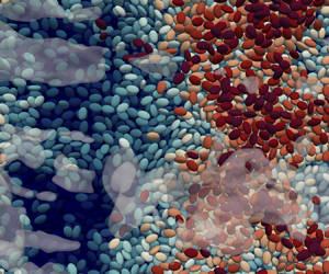
To assess qualitative differences in the collective particle behaviour resulting from the different shapes, figure 3 provides top views of instantaneous particle bedforms for all cases. Marked qualitative differences are observed in terms of the wavelength of the pattern, as well as differences in the mean sediment-bed height ( $H_{sed}/D_{eq}$) which are reported in table 1.

Figure 3. Snapshots of the bedforms obtained with the different particle shapes viewed from the top at an arbitrary instant in time: (a) Zingg ellipsoid, (b) prolate, (c) oblate and (d) spherical particles. The colour scale corresponds to the elevation of the centre point of a particle.
Another viable perspective is provided by figure 4 showing the space–time correlation  $R_{st} (r_x, \delta t)$ for all cases. This quantity is defined as
 \begin{equation} {R_{st} (r_x, \delta t) = \frac{\langle h'_{s} (x, t_{in}) h'_{s} (x+r_x, t_{in}+\delta t) \rangle_x}{\sqrt {\langle h'^2_{s}(x, t_{in}) \rangle_x \langle h'^2_{s} (x+r_x, t_{in}+\delta t) \rangle_x}} , {}} \end{equation}
where  $r_x$ and $\delta t$ are lags in space and time, respectively. The quantity $h'_{s}$ represents the spatial fluctuations in the spanwise averaged sediment-bed height.

Figure 4. The space–time correlation of fluctuations in the sediment-bed height in case (a) Zingg ellipsoid, (b) Prolate, (c) Oblate and (d) Sphere.
The simulation with spherical particles yields one cluster, more noticeable in figure 4(d) than in figure 3(d). Performing dune-conditioned averaging with a method described in Jain, Tschisgale & Fröhlich (Reference Jain, Tschisgale and Fröhlich2019b) an average amplitude of  $0.8D_{eq}$ was obtained. In the simulations of Kidanemariam & Uhlmann (Reference Kidanemariam and Uhlmann2017) with spherical particles dune-like structures were observed with an amplitude approximately equal to $2D_{eq}$. There, a fully developed cluster was observed after $316 H/ U_{b}$, whereas in the present study a total period of approximately $550 H/ U_{b}$ was simulated, which is longer and ensures that enough time was given for the pattern to develop. The difference in amplitude, instead, is likely to be related to the different Galilei numbers. In the present study $D_{eq}^+=16.4$ which is larger by a factor of about $1.6$ compared to Kidanemariam & Uhlmann (Reference Kidanemariam and Uhlmann2017), and $Ga=44.7$ which is $1.5$ times larger than the value in that reference. Another important difference is the submergence height. The water depth $H/D_{eq}$ in the simulations of Kidanemariam & Uhlmann (Reference Kidanemariam and Uhlmann2017) is $1.4$ times the submergence in the current simulation. Finally, the restitution coefficient in that reference is $0.3$, which is less than one third of the present value. In summary, the differences in the results are generated by differences in the regimes simulated. In the cases with non-spherical particles seen in figure 3 the amplitude of the bedform waviness is higher than in the case Sphere. The former feature very clear spanwise oriented dune-like structures of different size and distance for different particle shapes. The cluster present in the case Oblate is the largest among all, and the particle elevation is much larger than in the other cases. In the cases Zingg ellipsoid and Prolate zones of dark blue colour, i.e. $y < 3D_{eq}$, are visible. Animations show that here a fast downward-moving fluid structure displaces the particles. The bedforms differ markedly, without a monotonic dependency on the aspect ratio $a : c$, for example. As shown in figure 4, the propagation of the maximum correlation in space and time clearly differs between the simulations. The information such as pattern wavelength or the bedform celerity hidden in these plots should be interpreted with caution because of the limited domain size used in this study. However, the inherent difference in the bedform caused solely by the change in the particle shape is very noticeable.
4.2. Average packing fraction and particle velocities
Figure 5(a) displays the porosity  $\langle \phi \rangle$. Here, a porosity of $90\,\%$ is identified with the mean bed height (Kidanemariam & Uhlmann Reference Kidanemariam and Uhlmann2017) and indicated with a symbol in these and the following profiles. For the case with spherical particles $\langle \phi \rangle \approx 0.4$ up to $y = 3.5 D_{eq}$. The value of porosity encountered amounts to a packing fraction, $1-\langle \phi \rangle \approx 0.6$. Corresponding experimental values are $0.55 \ldots 0.62$ (Aussillous et al. Reference Aussillous, Chauchat, Pailha, Médale and Guazzelli2013) and $0.585 \pm 0.002$ (Boyer, Guazzelli & Pouliquen Reference Boyer, Guazzelli and Pouliquen2011), so that the present result is in very good agreement. The current packing fraction is not too far from the packing fraction which corresponds to the maximally jammed state of monodisperse spherical particles, i.e. $\approx 0.64$ (Scott & Kilgour Reference Scott and Kilgour1969; Torquato, Truskett & Debenedetti Reference Torquato, Truskett and Debenedetti2000). As a result, particle movement is substantially reduced, as seen in figure 5(b), where $\langle u_{p} \rangle \approx 0$ for $y < 4D_{eq}$ in the case Sphere. The packing fractions in the cases Zingg ellipsoid and Prolate are similar to the former case for $y < 4D_{eq}$. The average particle velocity, on the other hand, is slightly positive in the upper part of the bed indicating lower jamming.

Figure 5. Wall-normal profiles of mean quantities related to the particle movement: (a) mean porosity, (b) mean streamwise velocity and (c) mean angular velocity in spanwise direction. The markers identify the position  $y = H_{sed}$ with $\langle \phi \rangle = 0.9$ in all cases. Note the smaller vertical range in (b) and (c) to focus on regions of particle presence, $\langle \phi \rangle < 0.999$.
The smallest packing fraction of about  $0.4$ in this region is obtained in the case Oblate. Donev et al. (Reference Donev, Cisse, Sachs, Variano, Stillinger, Connelly, Torquato and Chaikin2004) reported packing fractions between $0.68$ and $0.71$ for jammed oblates with an aspect ratio close to $b/c \approx 2$, so that only about 60 % of this value is obtained in the simulation of the sediment constituted of oblates, here. This coincides with larger particle velocities (figure 5b) and quantifies the fact that the arrangement of particles in the moving sediment is far from the limit found by purely geometrical considerations.
Furthermore, the oblates are transported by the flow at much higher elevations than the other particles investigated, as seen by the smaller values of  $\langle \phi \rangle$ for $y>5D_{eq}$. At $y = H_{sed}$, oblates have the largest streamwise velocity from all cases, followed by the spherical particles. However, at $y = H_{sed}+2D_{eq}$, the spherical particles move fastest. The streamwise velocities in the cases Prolate and Zingg ellipsoid are similar.
Figure 5(c) shows the spanwise component of the mean angular velocity of the particles. The spherical particles have the largest value of  $\omega _{p,z}$ and the oblate spheroids the smallest. These results, combined with figure 5(b), indicate that the spherical particles predominantly roll, whereas oblate spheroids slide with little rotation. Considering few particles transported over a rough wall (Jain et al. Reference Jain, Tschisgale and Fröhlich2019c) reported that the oblate spheroids do not roll but align horizontally with their maximum projected area. Such preferential orientation has also been noticed in a case of non-buoyant particles by Ardekani et al. (Reference Ardekani, Costa, Breugem, Picano and Brandt2017) and Eshghinejadfard, Zhao & Thévenin (Reference Eshghinejadfard, Zhao and Thévenin2018), for example. The prolate spheroids and the Zingg ellipsoids exhibit rotation rates between the two extreme cases.
4.3. Mean shear stress and its contributions
The volume force,  $\langle \,f_{v} \rangle _t$, applied to impose the constant bulk Reynolds number in a simulation, must be balanced by the total shear stress in the system which, in turn, is the sum of viscous shear stress, Reynolds shear stress and stress due to the no-slip condition at the particle surface (Kidanemariam & Uhlmann Reference Kidanemariam and Uhlmann2017). The mean total shear stress is calculated using an approach proposed by Nikora et al. (Reference Nikora, McEwan, McLean, Coleman, Pokrajac and Walters2007) evaluating
 \begin{equation} \tau_{tot} = \rho_{f} \langle \,f_{v} \rangle_t \int_{y}^{L_y} \langle \phi \rangle ({y}) \, \textrm{d}{y} = \rho_{f} \nu_{f} \partial_y \langle u \rangle -\rho_{f} \langle u'v' \rangle + \tau_{\varOmega_{p}} , \end{equation}
where  $\tau _{\varOmega _{p}}$ is the stress contribution by the fluid–particle interaction. The wall shear stress is then defined setting $\tau _{w}=\tau _{tot}(y=H_{sed})$. The profiles of the total shear stress and all three individual contributions are shown in figure 6. The total shear stress, $\tau _{tot}$, is larger for the non-spherical compared with the spherical particles, largest for case Prolate. The wall shear stress obtained in the simulation with prolates is $1.6$ times the value for the case Sphere. In general, the mean sediment transport rate, $\langle Q_{p} \rangle _t$, is expressed as a function of ${Sh}$, which is proportional to $\tau _{w}$. Among the current simulations, however, the case Oblate has the largest sediment transport rate, despite not having highest $\tau _{w}$, which again highlights the importance of the particle shape. The maximum viscous shear stress is highest in the case Sphere which is approximately $2.75$ times the maximum value for the oblate spheroids (figure 6b). The profiles of the Reynolds shear stress are similar to the wall-normal Reynolds stress, being largest in the case of prolate spheroids and smallest in the case of spherical particles. Below $y = 5 D_{eq}$, $\tau _{\varOmega _{p}}$ is smallest in the case Sphere compared with the non-spherical particles, which is expected since the spheres have the smallest surface area. Interestingly, $\tau _{\varOmega _{p}}$ is not the largest in the case Oblate despite their largest surface area. This is due to the smaller solid volume fraction $(1-\langle \phi \rangle )$ in this region. Moreover, $\rho _{f} \nu_{f} \partial _y \langle u \rangle / \tau _{tot}$ is about $12\,\%$ in the case Sphere, whereas it is approximately $5\,\%$ in all other cases. The ratio $\rho _{f} \langle u'v' \rangle /\tau _{tot}$ is largest in the case Oblate, $65\,\%$ and $\tau _{\varOmega _{p}}/\tau _{tot}$ is largest in the cases Zingg ellipsoid and Prolate, $46\,\%$.

Figure 6. Wall-normal profile of the total shear stress and its different contributors: (a) total shear stress, (b) viscous contribution,  $\nu \partial _y \langle u\rangle /U^2_{b}$, (c) Reynolds shear stress, $\langle u'v' \rangle /U^2_{b}$ and (d) shear stress due to fluid–particle interaction, $\tau _{\varOmega _p}/(\rho _{f}U^2_{b})$. (Line style same as in figure 7).
The contribution of the grain-scale shear stress  $\tau _{\varOmega _{p}}$, which is caused by the fluid–particle interaction, is generally modelled as a function of the particle volume concentration only (e.g.Chauchat et al. Reference Chauchat, Cheng, Nagel, Bonamy and Hsu2017). In the current simulations, the particle volume fraction at the fluid–sediment interface is the same, i.e. $1-\langle \phi \rangle = 0.1$, but the value of $\tau _{\varOmega _{p}}$ is different indicating that it is a function of particle shape as well.
4.4. Mean fluid velocity and Reynolds normal stresses
The inner region of the mean flow profiles over an immobile permeable rough bed can be divided into three layers (Nikora et al. Reference Nikora, Goring, McEwan and Griffiths2001). (i) The subsurface layer defined as the zone where  $d\langle \phi \rangle /{\textrm {d} y} \approx 0$ below the sediment–clear water interface with upper end $y_{s}$ (here threshold $0.01/D_{eq}$), (ii) the roughness layer between the top of the subsurface layer at $y_{s}$ and the bottom of the logarithmic layer at $y_{l}$, (iii) the logarithmic layer, where
 \begin{equation} \langle u \rangle = \frac{u_\tau}{\kappa} \ln \left( \frac{y-H_{sed}}{k_{s}} \right) + B_{s} , \end{equation}
with  $\kappa = 0.4$ the von Kármán constant, $k_{s}$ the granular roughness and $B_{s}$ the roughness function which depends upon $k^{+}_{s}$ and was determined according to the relation provided in da Silva & Yalin (Reference da Silva and Yalin2017).
4.4.1. Subsurface layer
In case Sphere,  $y_{s} = 3.5D_{eq}$ and the small porosity in this region, close to the jamming state, leads to an almost vanishing fluid velocity. The porosity is slightly higher in the cases of prolate spheroids and Zingg ellipsoids due to the particle shape providing more pore space for fluid movement. A clear subsurface layer is not observed in the simulation with oblate spheroids.
4.4.2. Roughness layer
This layer is composed of form-induced sublayer and interfacial sublayer where saltating particles and various bedforms interact with the fluid (Nikora et al. Reference Nikora, Goring, McEwan and Griffiths2001). Its thickness is smallest in case Sphere,  $3.4D_{eq}$, while extending up to $y_{l} = 8.9D_{eq}$ with the oblates. The roughness layer obtained with the Zingg ellipsoids and the prolate particles has a thickness of $5D_{eq}$ and $4.5D_{eq}$, respectively. The fluid velocity at the interface between the roughness layer and the logarithmic layer is largest with the oblates and smallest with the prolate spheroids.
4.4.3. Logarithmic layer
The wall-normal profile of the streamwise fluid velocity in wall units is shown in figure 7(b). The value of  $k_{s}$ was chosen such that (4.3) provides the best fit to the mean streamwise velocity profile in the logarithmic region (error less than $5\,\%$). This profile is observed to hold for $(y-H_{sed})^+ \gtrsim 30$. Often it is seen that this behaviour reaches until $20\,\%$ of the submergence (da Silva & Yalin Reference da Silva and Yalin2017), but in the present simulations the wake is barely pronounced, so that the fit is satisfactory almost up to the free surface. The corresponding equivalent roughness thickness $k_{s}$ equals ${4.3}{D_{eq}}$, ${5.1}{D_{eq}}$, ${3.2}{D_{eq}}$ and ${2.6}{D_{eq}}$ in the cases Zingg ellipsoid, Prolate, Oblate and Sphere, respectively. The corresponding roughness Reynolds number for each case is listed in table 1. The change in the equivalent roughness thickness caused by the particle shape again highlights its importance. Figure 7(c) shows the particle relative velocity $\langle u_{r} \rangle = \langle u_{p} \rangle - \langle u \rangle$. Among all cases, $\langle u_{r} \rangle$ at $y = H_{sed}$ is largest for prolate spheroids. The profiles of the relative velocity in the non-spherical cases have their maximum value at $y \approx H_{sed}+D_{eq}$, compared with $y \approx H_{sed}$ for spheres. As in figure 5, Prolate and Zingg ellipsoid yield very similar results, the difference with respect to the other two cases exceed $100\,\%$ of the latter. The Reynolds normal stresses are shown in figure 8. The streamwise component differs substantially, being largest with the prolate and smallest in the case of oblate spheroids, having their maximum value slightly above $H_{sed}$. The profiles of $\langle v'v' \rangle$ and $\langle w'w' \rangle$ exhibit similar differences, with their respective maximum attained well above $H_{sed}$. Below $y \approx 3 D_{eq}$, the simulation with oblates has much larger fluctuations compared with the others because of the substantially higher porosity (figure 5a), whereas the normal stresses are almost zero for spherical particles in this region. The larger permeability in the case Oblate also seems to be the reason for the smaller maximum values in this case. Blois et al. (Reference Blois, Best, Sambrook, Gregory and Hardy2014) and Sinha et al. (Reference Sinha, Hardy, Blois, Best and Sambrook Smith2017) found that the turbulence intensity in the channel decreases with increasing permeability yielding increased subsurface flow.

Figure 7. Mean fluid streamwise velocity profiles: (a)  $\langle u \rangle$ in bulk units, (b) $\langle u \rangle$ in wall units, solid blue line represents (4.3) for case Prolate with $k_{s} = 5.1$ (no dots at $y-H_{sed} = 0$ due to logarithmic axis) and (c) mean relative velocity, $\langle u_{r} \rangle = \langle u_{p} \rangle - \langle u \rangle$, normalised with $U_{b}$.

Figure 8. Wall-normal profiles of the averaged Reynolds normal stresses normalised with the bulk velocity: (a) streamwise component  $\langle u'u' \rangle /U^2_{b}$, (b) wall-normal component $\langle v'v' \rangle /U^2_{b}$ and (c) spanwise component $\langle w'w' \rangle /U^2_{b}$. (Line style as in figure 7).
5. Conclusions
Three DNS with non-spherical particles were conducted, complemented by a fourth case with spherical particles. The set-up was thoroughly devised to allow a well-controlled, systematic study of the influence of the particle shape on the fluid and particle statistics. Ample statistical data were reported quantitatively, assessing substantial differences resulting from a change of particle shape only. For example, the sediment of spherical particles has the largest solid volume fraction, in fact, it is close to the jammed packing fraction of randomly arranged spheres, so that the movement of particles and fluid in the sediment is extremely hindered. On the other hand, the sediment bed composed of oblates is very permeable which allows a much easier movement of fluid and particles below the sediment–fluid interface.
The mean sediment transport rate is not largest in the case Prolate, even though the non-dimensional shear stress is highest in this case. Similarly, in the case Oblate the value of  $\langle Q_{p} \rangle _t$ is maximum, although the bottom shear stress is not largest due to a considerable subsurface flow which substantially reduces turbulence in the channel. The results also show that the bedforms are highly influenced by the particle shape. We recommend further studies on the impact of the particle shape on pattern evolution and bedload characteristics. Overall, the data reported here constitute reference data for future studies, numerical or experimental, as they are rich in information and lend themselves for further physical exploitation and modelling. In particular, closure assumptions with the scaling laws accounting for the particle shape mentioned in the introduction can be assessed and possibly amended with the present data.
Supplementary movies
Supplementary movies are available at https://doi.org/10.1017/jfm.2021.214.
Acknowledgements
The simulations were carried out at the ZIH, TU Dresden. R.J. thanks L. Sachsen for providing the scholarship, No. L-201535.
Declaration of interests
The authors report no conflict of interest.


 Open access