


1 Introduction
The ever-increasing product complexity continues to provide challenges in the management of product dependencies with conflicts and constraints needing to be resolved on a daily basis. Failure to do so can lead to costly overruns and considerable re-work. Examples include issues in the length of cabling required in the A380, resulting in a $6.1 billion delay and faulty hybrid software resulting in Toyota recalling 625,000 vehicles (Calleam 2011; Bruce Reference Bruce2015). This has led to a growing consensus that current project management strategies (which date back to the 1950–1980s) are beginning to be overwhelmed by the complex, multi-disciplinary and distributed nature of modern engineering projects (Beitz et al. Reference Beitz1986; Linick and Briggs Reference Linick and Briggs2004).
Having identified this challenge, researchers have developed new methods and tools that provide more pro-active and real-time design and project management support by utilising the ever-growing digital footprint of engineering projects (Gopsill et al. Reference Gopsill, Shi, McMahon and Hicks2014; Snider et al. Reference Snider, Shi, Jones, Gopsill and Hicks2015, Reference Snider, Gopsill, Jones, Emanuel and Hicks2019). For example, the development of the Boeing 787 Dreamliner involved the production of over 300,000 computer aided design (CAD) models, which were accessed between 75,000 and 100,000 times a week (Briggs Reference Briggs2012). However, Jones et al. (Reference Jones, Xie, McMahon, Dotter, Chanchevrier and Hicks2016) study on the search and retrieval behaviour of employees at Airbus revealed that engineers performed 1.1 million searches for information over a six-month period. This continually increasing repository of engineering project digital footprints provides the potential for comparison of engineering digital work to reveal emergent structures (ES) in engineering project behaviour. These structures could relate to best practice, normal behaviour and potential issues within engineering projects, and the identification and subsequent coding of these structures would lead to insights that could support the management of future engineering projects. Although logical, there remains a lack of studies investigating whether ES can be determined through cross-project comparison and the development of methodologies to perform such investigations.
This paper fills this gap by contributing a study that compares the digital footprints of a set of near-identical systems design projects (Formula Student (FS)) to investigate the existence of ES of engineering project behaviour.
This has been achieved by the following:
(1) generating dynamic design structure matrices (DSMs) from the record of file edits;
(2) generating hypotheses as to the potential ES from the design intent and competition performance of the teams;
(3) mapping and identifying ES through comparison of the dynamic DSMs and ES hypotheses.
The paper continues by discussing the related work (Section 2), which covers the definition of DSMs, state-of-the-art in dynamic DSMs and rationale for their selection as the technique for the comparison. Section 3 describes the method used to generate the dynamic DSMs used in this study. With this grounding, Section 4 discusses the near-identical FS systems design projects where hypotheses on the ES are developed. This then continues into the application of dynamic DSMs (Section 5). Section 6 presents the results of the dynamic DSMs where the focus has been on comparing the three teams and mapping the results to hypotheses. These are then discussed along with the future work that could be performed (Section 7). The paper then concludes by highlighting the key contributions of the paper (Section 8).
2 Related work
DSMs were originally developed in the 1980s by Steward (Reference Steward1981) as a branch of graph theory; DSMs seek to understand the connected nature of engineering systems through an $N\times N$
matrix of interactions between system elements (Eppinger Reference Eppinger1997). Since then, they have been widely applied as a means to identify, visualise and monitor product and organisational architectures (Browning Reference Browning2016; Sosa, Eppinger & Rowles Reference Sosa, Eppinger and Rowles2003). These systems can represent individual components, assemblies of components, systems of components, engineers, teams of engineers, processes and/or organisational structures, with the level of interactivity between elements being manually scored using ordinal, categorical or binary data (Sosa et al.
Reference Sosa, Eppinger and Rowles2003; Gorbea et al.
Reference Gorbea, Spielmannleitner, Lindemann and Fricke2008). Partitioning and matrix visualisation techniques are then applied to produce insights on the product/organisational architecture.
$N\times N$
matrix of interactions between system elements (Eppinger Reference Eppinger1997). Since then, they have been widely applied as a means to identify, visualise and monitor product and organisational architectures (Browning Reference Browning2016; Sosa, Eppinger & Rowles Reference Sosa, Eppinger and Rowles2003). These systems can represent individual components, assemblies of components, systems of components, engineers, teams of engineers, processes and/or organisational structures, with the level of interactivity between elements being manually scored using ordinal, categorical or binary data (Sosa et al.
Reference Sosa, Eppinger and Rowles2003; Gorbea et al.
Reference Gorbea, Spielmannleitner, Lindemann and Fricke2008). Partitioning and matrix visualisation techniques are then applied to produce insights on the product/organisational architecture.
Figure 1 shows the results of a DSM analysis that was used to uncover the dependencies within a commercial jet engines’ product architecture. The study revealed a disparity between the product and organisational architectures, which was not known to the engineers at the time. Providing this information to the project managers led to a re-organisation of the team structure and an increase in productivity.

Figure 1. A DSM of a commercial jet engine (Sosa et al. Reference Sosa, Eppinger and Rowles2003).
While insightful, the established methods for capturing the primary dataFootnote 1 lead to challenges in being able to maintain DSMs that are representative of the current state of a design. To illustrate, the generation of the DSM for a timber construction company was achieved through an iterative interview and survey approach that involved employees working on 60 timber structure projects over a six-month period (Björnfot & Stehn Reference Björnfot and Stehn2007). In addition, challenges in the consistency of the data format used have also been raised with researchers investigating data exchange formats to enable the sharing and comparison of DSMs across the field (Ansari et al. Reference Ansari, Hossain and Khan2016). The limitations of the established manual generation methods have been further confirmed by the Browning (Reference Browning2016) review of DSM research, which concludes that there are two major challenges for future DSM research:
(1) the large amount of new data required to build a rich, structural model of some systems;
(2) the absence of a versatile and user-friendly software tool set for DSM modelling, manipulation and analysis.
The review also highlights that the established manual generation methods are ‘tedious and error-prone’ leading to a barrier in gaining full stakeholder engagement and increases uncertainty in the quality and accuracy of the resulting DSM.
To overcome the limitations of the current generation methods, researchers have begun to investigate how the output of engineering work can be used to elicit the connected nature of system components (Morkos, Shankar & Summers Reference Morkos, Shankar and Summers2012; Senescu et al. Reference Senescu, Head, Steinert and Fischer2012; Gopsill et al. Reference Gopsill, Snider, McMahon and Hicks2016). Examples include the tracking of file exchanges between individuals (Senescu et al. Reference Senescu, Head, Steinert and Fischer2012), aggregation and processing of change request documents (Morkos et al. Reference Morkos, Shankar and Summers2012; Ghlich, Hildebrand & Schellert Reference Ghlich, Hildebrand and Schellert2018) and the capture of file edit co-occurrences to build a probabilistic model of dependencies (Gopsill et al. Reference Gopsill, Snider, McMahon and Hicks2016). Each has the potential to provide a more automated, system agnostic, objective and real-time method that results in the generation of DSMs that are in line with the evolution of the project. The resulting DSMs are herein referred to as dynamic DSMs.
To validate dynamic DSMs, Gopsill et al. (Reference Gopsill, Snider, McMahon and Hicks2016) used the CAD system structural dependencies (i.e. part, sub-assembly, assembly trees) as a ground truth and revealed that their probabilistic model of dependencies produced from the co-occurrence of file edits was able to not only identify the structural dependencies but also dependencies relating to the function of the product and design process. Subsequent post-processing of the DSM was also able to identify the likely change propagation characteristics of models.
Although research has been performed to generate and verify these new methods of generating dynamic DSMs, there has yet to be a study that has used these techniques to compare design projects and to see whether ES of digital work exist. Thus, this paper moves the DSM field forward by providing such an analysis on a set of near-identical systems design projects.
3 Dynamic DSM generation
Dynamic DSMs is the term used for methods that generate DSMs that reflect the dependencies within an engineering project in real time. The theoretical model used in this paper is Gopsill et al. (Reference Gopsill, Snider, McMahon and Hicks2016) conditional probability model, which is based on the co-occurrence of file edits.
In this model, it is posited that files edited within a pre-defined time period of one another are candidates for a potential dependency. The likelihood of this dependency being true, alongside the potential strength of this dependency, is increased by a consistent re-occurrence of this file edit behaviour. Coupled with the understanding that there are hundreds of thousands of file edits occurring and the resulting low probability of a consistent re-occurrence of file edit behaviour developing, any consistent behaviour observed is likely to relate to a dependency of some description. Examples of consistent re-occurring file edit behaviours include the editing of a part file and subsequent update of an assembly and the systematic generation and subsequent editing of temporary files during simulation runs. In the case of the latter, these can be determined through the consistency in the timings of file edits and subsequently coded as dependencies within the simulation process.
A particular affordance of this model is that it relies solely on file edit timestamps. These are a ubiquitous source of information that is captured by server and product data management systems. Thus, the use of this type of information enables DSMs to be generated independently of the product lifecycle management architecture, thereby increasing the applicability of the model and reducing IP/security concerns as no file content is analysed.
The implementation of this model requires the generation of an $N\times N$
matrix that represents the co-occurrence of file edits between files within the engineering project. This is subsequently post-processed to uncover the dependencies and key modules of the project/product depending on the sub-set of files used. The implementation comprises seven stages and covers the following:
$N\times N$
matrix that represents the co-occurrence of file edits between files within the engineering project. This is subsequently post-processed to uncover the dependencies and key modules of the project/product depending on the sub-set of files used. The implementation comprises seven stages and covers the following:
(1) File selection
(2) Generation
(3) Evaluating ‘directedness’
(4) Normalisation
(5) Pruning
(6) Partitioning
(7) Optimisation
The paper continues by describing Stages 1–7. For a more in-depth discussion of the process, please see Gopsill et al. (Reference Gopsill, Snider, McMahon and Hicks2016). The paper also uses a number of matrix analysis definitions. To ensure clarity, their definitions with respect to this context are as follows:
- Partition
– A grouping of highly interdependent files whilst maintaining dependencies to other groups of files. These represent modules within a product/project.
- Components
– A grouping of highly interdependent files that are not dependent on other partitions/components within the DSM. These represent distinct modules where changes are highly unlikely to require further changes to additional modules within the product/project.
- Modularity
– A normalised metric (0–1) that indicates the level of structure within the matrix that is beyond pure chance. Values greater than $0.3$
are often considered a good indicator for the capture of dependencies between nodes (Newman Reference Newman2004).
$0.3$
are often considered a good indicator for the capture of dependencies between nodes (Newman Reference Newman2004).

3.1 File selection
Stage 1 of the process requires the specification of the files to be analysed. This depends on the engineering project and dependencies between the files one wishes to investigate. Examples include the use of CAD files to determine product dependencies and emails to determine process dependencies.
With the files selected, a further thresholding of the files is performed based on file activity. At this initial stage, a file activity of greater than four updates is often chosen. This represents the creation followed by three more edits to the file.
The aim is to remove the files that show little to no activity and, thus, may represent areas of the product/project that cannot be altered by the team (e.g. a bought-in part such as the engine block and/or gearbox). Imposing a low threshold for the number of files helps prevent an overreduction in the size of dataset; however, too low and a probabilistic model cannot be achieved as there is a lack of edits to build up confidence in the candidate dependencies.
3.2 Generation
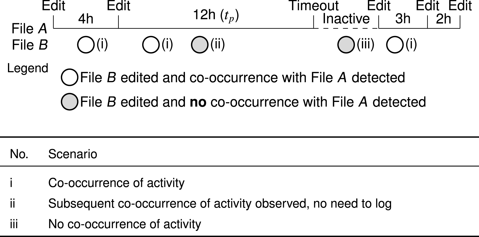
Figure 2. Detecting co-occurrences of file edits.
To generate the co-occurrence DSM, one needs to identify when a co-occurrence of file activity has occurred. To achieve this, the process iterates through each file edit timestamp and identifies the files that have changed within a specified time period. The matrix is then updated to reflect the frequency of the co-occurrence of edits between the files.
Figure 2 illustrates the process of identifying the co-occurrence of file edits. Taking File A as the file of interest, the process identifies all the timestamps where the file has changed and generates the time periods where the occurrence of edits to other files are retrieved. $t_{p}$
defines the maximum time period post a file edit and can often be smaller due to A being edited again within this period. This is demonstrated in Figure 2 where
$t_{p}$
defines the maximum time period post a file edit and can often be smaller due to A being edited again within this period. This is demonstrated in Figure 2 where $t_{p}$
is set to 12 h, but 4, 3 and 2 h are present due to additional edits being made to A. Dynamically adjusting the time period ensures no double counting of file edit co-occurrences.
$t_{p}$
is set to 12 h, but 4, 3 and 2 h are present due to additional edits being made to A. Dynamically adjusting the time period ensures no double counting of file edit co-occurrences.
With the time periods for a co-occurrence with respect to A defined, one can now refer to the edit timestamps for the other files and check whether a co-occurrence has occurred. Figure 2 shows the three possible scenarios. Scenario (i) occurs where File A has changed and File B changes within the post-edit time period. This leads to a co-occurrence of file activity being recorded. Scenario (ii) occurs where File B changes again within the same post-edit time period. Since a co-occurrence has already been recorded, no further co-occurrences are recorded. Scenario (iii) occurs where File B changes within a period of inactivity of File A. In this case, there is no co-occurrence of file activity.
This results in a matrix consisting of the number of file edit co-occurrences. This is taken to Stage 3, which normalises the matrix with respect to the number of edits to the files.
3.3 Normalisation
At this stage, the process has generated a DSM consisting of the number of file edit co-occurrences. If one would partition the current DSM, the resulting partitions would be highly influenced by the files with a high number of edits.
Thus, normalisation against the number of edits is performed to adjust for the unequal distribution of edits across the files. To do this, the process applies conditional probabilities. Referring back to the theoretical model, this is the assessment of the consistency of file edit co-occurrences and is achieved by taking the number of co-occurrences between two files $u$
and
$u$
and $v(C_{u,v})$
and dividing it by the total number of edits of
$v(C_{u,v})$
and dividing it by the total number of edits of $u(E_{u})$
to give the probability of an edit in
$u(E_{u})$
to give the probability of an edit in $u$
leading to a co-occurrence edit in
$u$
leading to a co-occurrence edit in $v(P_{u,v})$
. This is shown in the following equation:
$v(P_{u,v})$
. This is shown in the following equation:
 $$\begin{eqnarray}P_{u,v}=\frac{C_{u,v}}{E_{u}},\end{eqnarray}$$
where $P_{u,v}$
is the conditional probability of an edit in
$P_{u,v}$
is the conditional probability of an edit in $u$
post
$u$
post $v$
,
$v$
, $C_{u,v}$
is the number of co-occurrences between
$C_{u,v}$
is the number of co-occurrences between $u$
and
$u$
and $v$
and
$v$
and $E_{u}$
is the number of edits to file
$E_{u}$
is the number of edits to file $u$
.
$u$
.
The result of this normalisation is a directed DSM that represents the conditional probabilities of a dependency between the files. To continue, the process evaluates the ‘directedness’ of the DSM to determine whether a directed or undirected DSM should be used and the appropriate partitioning technique is applied.
3.4 Evaluating the ‘directedness’
Up until this point, the DSM has been inherently directed where a change in the file in the row vector $(u)$
has a likelihood of leading to a change in the file in the column vector
$(u)$
has a likelihood of leading to a change in the file in the column vector $(v)$
. This ‘directedness’ (
$(v)$
. This ‘directedness’ ( $D$
) is subsequently analysed to assess its significance in order to ensure that the appropriate directed or undirected partitioning techniques are applied (Equation (2)). This is evaluated by taking the average of the absolute differences in the conditional probabilities between the files within the DSM. If
$D$
) is subsequently analysed to assess its significance in order to ensure that the appropriate directed or undirected partitioning techniques are applied (Equation (2)). This is evaluated by taking the average of the absolute differences in the conditional probabilities between the files within the DSM. If $D$
is close to
$D$
is close to ${<}0.1$
, then it is argued that no significant directionality exists within the DSM.
${<}0.1$
, then it is argued that no significant directionality exists within the DSM.
 $$\begin{eqnarray}D=\frac{\sum \unicode[STIX]{x1D6E5}P_{u,v}}{\sum E}=\frac{\sum |(P_{u,v}-P_{v,u})|}{\sum E}.\end{eqnarray}$$
As the focus of this paper is not to discuss the process entirely, the paper will focus on the analysis of undirected matrices as this was found to be the case for the systems design projects to be compared. Equation (3) details the transformation from a directed to undirected matrix $(U_{u,v})$
, which takes the average of the two directed conditional probabilities
$(U_{u,v})$
, which takes the average of the two directed conditional probabilities $(P_{u,v},P_{v,u})$
.
$(P_{u,v},P_{v,u})$
.
 $$\begin{eqnarray}U_{u,v}=U_{v,u}=\frac{P_{u,v}+P_{v,u}}{2}.\end{eqnarray}$$
With the DSM normalised and directionality determined, the process moves to the pruning of the DSM where further noise is removed from the DSM ahead of performing the partitioning.
3.5 Pruning
The objective of pruning is to omit candidate dependencies that are a likely result of randomness and concurrency of engineering work. In addition, this reduces the computational time taken to partition and analyse the DSM by increasing the spareness of the matrix. This enables the DSM to be maintained and updated in real time as the project evolves. Pruning is the act of running through all the candidate dependencies and removing any that are below a defined pruning value $(p)$
. The optimum value for
$(p)$
. The optimum value for $p$
is generated during Stage 7 (Section 5.8). Pruning the matrix also has the ability to disconnect files and groups of files from the rest of the matrix. In the first case, the process removes this file from the rest of the analysis, while in the second case, the group of files remain within the matrix, thereby forming components. With the pruning complete, the co-occurrence DSM is ready to be partitioned to uncover the underlying and evolving architecture of the engineering project.
$p$
is generated during Stage 7 (Section 5.8). Pruning the matrix also has the ability to disconnect files and groups of files from the rest of the matrix. In the first case, the process removes this file from the rest of the analysis, while in the second case, the group of files remain within the matrix, thereby forming components. With the pruning complete, the co-occurrence DSM is ready to be partitioned to uncover the underlying and evolving architecture of the engineering project.
3.6 Partitioning
Partitioning reveals the DSM’s underlying structure. While there are many algorithms that could be applied to reveal the underlying structure of the DSM, this paper applies the Louvain community partitioning algorithm (Blondel et al. Reference Blondel, Guillaume, Lambiotte and Lefebvre2008). This algorithm is typically applied to communication transactions, such as email and social media, to reveal communities within social networks. As the co-occurrence measurements used to form the DSMs are also of a continuous and transactional form, it is argued that the partitioning algorithm will also be suitable for this case.
The algorithm works by allocating files to partitions with the objective of returning a partition set that produces the highest modularity score for the DSM. Modularity ( $Q$
) is an assessment of the quality of the matrix partition and is defined as (Newman Reference Newman2004)
$Q$
) is an assessment of the quality of the matrix partition and is defined as (Newman Reference Newman2004)
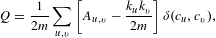 $$\begin{eqnarray}Q=\frac{1}{2m}\mathop{\sum }_{u,v}\left[A_{u,v}-\frac{k_{u}k_{v}}{2m}\right]\unicode[STIX]{x1D6FF}(c_{u},c_{v}),\end{eqnarray}$$
where $m=\frac{1}{2}\sum _{u,v}A_{u,v}$
and is the sum of the co-occurrences’ conditional probabilities within the matrix.
$m=\frac{1}{2}\sum _{u,v}A_{u,v}$
and is the sum of the co-occurrences’ conditional probabilities within the matrix. $\unicode[STIX]{x1D6FF}$
is the Kronecker delta function and is 1 if a co-occurrence exists between two files and 0 otherwise.
$\unicode[STIX]{x1D6FF}$
is the Kronecker delta function and is 1 if a co-occurrence exists between two files and 0 otherwise. $k_{u}k_{v}/2m$
is the probability that a co-occurrence may exist between two files, where
$k_{u}k_{v}/2m$
is the probability that a co-occurrence may exist between two files, where $k_{u}$
is the number of files that have co-occurrences with file
$k_{u}$
is the number of files that have co-occurrences with file $u$
and
$u$
and $k_{v}$
is the number of files that have co-occurrences with file
$k_{v}$
is the number of files that have co-occurrences with file $v$
. And
$v$
. And $A_{u,v}$
is the weighted co-occurrence between two files in the matrix.
$A_{u,v}$
is the weighted co-occurrence between two files in the matrix.
To start, the algorithm assigns each file to its own partition. The algorithm then sequentially moves one file to a different partition and calculates the change in modularity (Equation (5)).
 $$\begin{eqnarray}\unicode[STIX]{x1D6E5}Q=\left[\frac{P_{\text{in}}+k_{i,\text{in}}}{2m}-\left(\frac{P_{\text{tot}}+k_{i}}{2m}\right)^{2}\right]-\left[\frac{P_{\text{in}}}{2m}-\left(\frac{P_{\text{tot}}}{2m}\right)^{2}-\left(\frac{k_{i}}{2m}\right)^{2}\right],\end{eqnarray}$$
where $P_{\text{in}}$
is the sum of all the co-occurrence probabilities within the partition that file
$P_{\text{in}}$
is the sum of all the co-occurrence probabilities within the partition that file $i$
is being included in,
$i$
is being included in, $P_{\text{tot}}$
is the sum of all the co-occurrence probabilities to files within the partition that
$P_{\text{tot}}$
is the sum of all the co-occurrence probabilities to files within the partition that $i$
is being included in,
$i$
is being included in, $k_{i}$
is the co-occurrence degree of
$k_{i}$
is the co-occurrence degree of $i$
and
$i$
and $k_{i,\text{in}}$
is the sum of the co-occurrence probabilities
$k_{i,\text{in}}$
is the sum of the co-occurrence probabilities $i$
and other files within the partition that
$i$
and other files within the partition that $i$
is merging with.
$i$
is merging with.
From this, the maximum modularity change can be identified. The associated files are then assigned to the same partition and the algorithm repeats the previous step of identifying the next file movement that will result in a further increase in modularity. If no further movement of files achieves an increase in modularity, the algorithm terminates, resulting in the partition set that gives the highest modularity score. This iterative process results in a partition set that are highly connected internally and weakly connected to one another.
The process of generating the partition from the bottom-up makes the approach inherently hierarchical and maps well to the hierarchical nature of product architectures within CAD systems. Hence, it is suitable for analysing DSMs generated from the co-occurrence of edits to files.
3.7 Optimisation
With the generation process defined, Stage 7 optimises and evaluates the stability of the DSM partitioning as a function of time period $(t_{p})$
and pruning threshold
$(t_{p})$
and pruning threshold $(p)$
. The stage seeks to optimise for the following objective
$(p)$
. The stage seeks to optimise for the following objective $O$
function:
$O$
function:
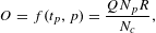 $$\begin{eqnarray}O=f(t_{p},p)=\frac{QN_{p}R}{N_{c}},\end{eqnarray}$$
where $Q$
is the modularity of the matrix partition,
$Q$
is the modularity of the matrix partition, $N_{p}$
is the number of matrix partitions,
$N_{p}$
is the number of matrix partitions, $R$
is the ratio of the matrix that remains after pruning and
$R$
is the ratio of the matrix that remains after pruning and $N_{c}$
is the number of matrix components.
$N_{c}$
is the number of matrix components.
To find the optimum values for $t_{p}$
and
$t_{p}$
and $p$
, a grid search using a range of time periods (0 to 24 h in increments of 1 h) and pruning values (0–1 in increments of 0.05) is used to generate the co-occurrence DSM and perform the partitioning. From this, the structural characteristics of each DSM are computed and
$p$
, a grid search using a range of time periods (0 to 24 h in increments of 1 h) and pruning values (0–1 in increments of 0.05) is used to generate the co-occurrence DSM and perform the partitioning. From this, the structural characteristics of each DSM are computed and $O$
is obtained. The values that produce
$O$
is obtained. The values that produce $O_{\max }$
are then selected as the optimum time period and pruning values. Further analysis of this grid search can also reveal the sensitivity of the identified structures and provide confidence in their significance to the project.
$O_{\max }$
are then selected as the optimum time period and pruning values. Further analysis of this grid search can also reveal the sensitivity of the identified structures and provide confidence in their significance to the project.
3.8 Summary
With the dynamic DSM method introduced, the paper now continues by describing the set of near-identical systems design projects, the dataset that has been generate and example process of applying the dynamic DSM generation method.
4 A set of near-identical systems design projects
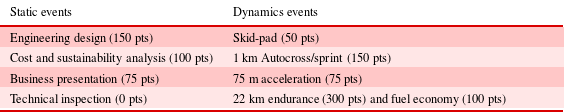
The sets of near-identical systems design projects that have been selected for the comparison are the annual FS projects run at the University of Bath. FS is a motor-sport educational programme where teams of students from universities compete in designing, building and racing a single-seat race car (Figure 3). It is an international competition with events held worldwide. The UK event has been running since 1999 with each team being judged on a mixture of dynamic and static events (Table 1).

Figure 3. Formula Student.
Table 1. FS competition events
Team Bath Racing have been designing and building FS cars for over a decade and consists of approximately 30 engineering students in their final year of study. A range of engineering courses including automotive, aerospace, electrical, manufacturing and mechanical engineering are represented by the team members and highlight the multi-disciplinarity of the project. The team have an allocated workspace and are provided with a shared network drive space where all the files pertaining to the car are stored and worked upon. Given the decades worth of experience in running the FS project, detailed design processes and product data management procedures (e.g., naming convention, check-in/out, version control and sign-off procedures) have been developed to support the team and are in line with industry best practice. In addition, Team Bath Racing are one of the few teams that design and build a car from scratch each year, and each member is required to do a final year project on an element of the car as part of their degree. The maturity of both the team and event and the consistency in the rules and judging provide a controlled environment where the design intent, competition performance and digital footprint can be captured and compared.
The following section details the design intent and competition performance. This will then be used during the comparison of the teams’ DSMs where evidence-based arguments will be made that map the ES within the DSMs to design intent and product performance.
4.1 Design intent
Table 2. FS team’s design intent as presented to the FS judges
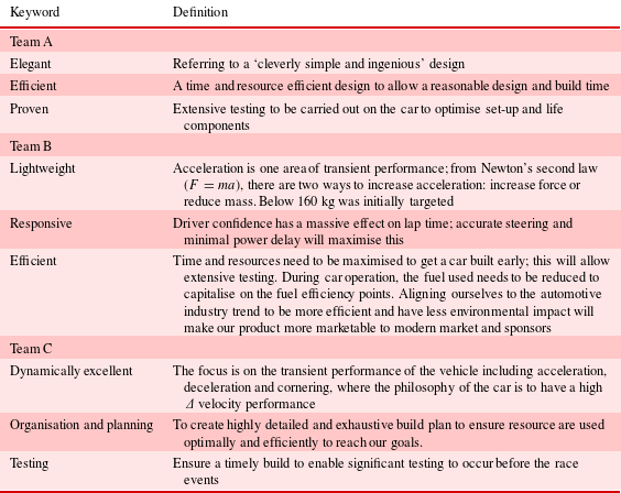
The design intent statements given to the FS judges by the three teams are presented in Table 2. From these statements, it can be seen that Team A’s design intent was centred on generating a reduced design cycle in order to allow for more time to be associated with the build and testing of the product. In contrast, Team B’s focus is on the transient performance and user-centred design of the vehicle alongside a rapid design cycle in order to increase time for building and testing. Team C further emphasises the importance of developing a car with good transient performance, and to achieve this, their aim is to have a highly detailed build plan that allows for significant time for testing.
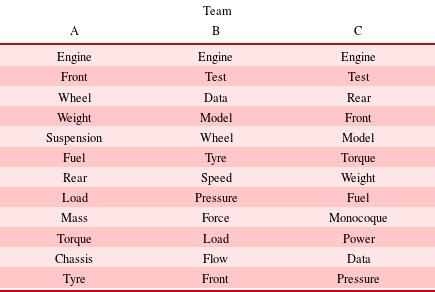
Table 3. Most common terms used across the team reports (in descending order)
In addition to the competition design and business reports, each engineer is required to produce a report on their work as part of a university assessment. Thus, the work discussed in these reports can provide an insight into the specific areas of focus for each team member and provides an indication of the allocation of resources across the design and manufacture of the car.
Natural language processing was applied to extract the commonly used terms across the reports. Stop-word lists were used to remove context independent terms from the analysis (e.g., the, a, and). Table 3 presents the top 12 terms for each team.
A consistent theme across all three teams is the importance of the engine in the development of the car. This is a logical outcome as the engine is integral to the power train and forms a central part of the chassis. Therefore, this is a crucial area for the team to understand in order for the rest of the car to be built.
Continuing down the list of terms, one can see the teams diverge due to their respective design intent. Team A focuses on wheel, weight, suspension, fuel, torque, chassis and tyres, which aligns with their intent of an ‘elegant’ design where they are wishing to create a simple robust design. These terms all relate to the fundamental principles of vehicle design and features of the car that have to exist in order for a car to function. The focus on simplicity is further highlighted by the lack of any terms relating to the aerodynamics and/or sensor data capture that one might expect on a racing car. Therefore, one would expect their DSM to have partitions centred around the chassis, suspension and wheel and tyres.
In contrast, Team B focuses on aerodynamics, data capture and testing with terms test, data, pressure and flow being used. In addition, model appears in the list, which highlights the greater use of digital modelling and simulation technologies used by Team B. Again, the set of terms aligns well to their design intent that focuses on being ‘lightweight’ and ‘responsive’ as it is argued that a considerable amount of modelling is required in order to understand how design concessions affect the transient performance of the car. Given the focus on testing, one would hypothesise that Team B’s DSM will be more modular to reflect the many tests that they wish to perform.
Team C appears to be an amalgamation of the previous two teams with a mix of fundamental features of the car such as weight, monocoque and power, whilst also considering the modelling and aerodynamics side of the car with the use of terms data, pressure and model. As the design intent of Team C is to be ‘dynamically excellent’, it can be argued that to achieve this, a team would need to be able to harmonise the fundamental chassis and suspension design with the additional loads generated by the supporting aerostructures. In addition, test is rated particularly high in Team C’s results, which further confirms the team’s focus on their design intent of ‘Testing’. Thus, it is hypothesised that Team C’s DSM would also contain more partitions to reflect testing and that the partitions will also centre around chassis and aerodynamic components.
This analysis of the teams’ design intent highlights that although each team is creating the same product, the approach each team has taken has had a considerable impact on the allocation of resources across the product architecture. Thus, there is potential in that similarities and differences can be observed in the comparison of DSMs for the FS teams and that structures within the DSMs may correspond to the design intent of the teams.
4.2 Product performance
Table 4. FS competition results
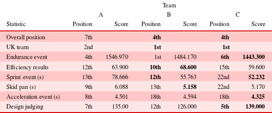
Table 4 presents the results from the FS competition and the hypothesis is that the comparison of DSMs may provide structures that indicate the potential performance of the final product.
In terms of overall position and top UK team, Teams B and C both outperform Team A with both teams placing 4th in their respective competition years. However, there is little difference in the UK team performance. Moving to the vehicle performance events, Team C outperformed Team A and B in the endurance event, which suggest that they were able to meet their design intent of ‘testing’ as reliability is the main concern for this event. Team B performed the best in efficiency and further confirms that they were able to translate their design intent of ‘efficient’ into the real-world product. However, in the sprint event, it is Team C that is the top performing team with a time of 52.232 s. This clearly aligns with their ‘dynamically excellent’ design intent.
Overall, Team C outperformed the other two teams at the competition; however, there were events that Team B did excel at. In contrast, whilst Team A did complete all the events of FS, their competition performance was not at the same level as Teams B and C. Therefore, there is potential for the study to uncover relationships in the DSM structures and overall competition and/or individual event performance.
4.3 Summary
From the discussion of both the teams’ design intent and product performance, the ES one hypothesises will exist within the DSMs are the following:
(i) Team A’s DSM partitions should be centred around the chassis, suspension and wheel and tyres.
(ii) Team A’s aim for an elegant and simple design will be reflected in a DSM with few disconnected modules.
(iii) Team B’s DSM is expected to be more modular to reflect the priority on testing the various systems of the car.
(iv) Team C’s DSM will contain more partitions to reflect the testing and that the partitions will also centre around chassis and aerodynamic components.
(v) Team C’s as-designed architecture revealed by the DSM will be more closely aligned to their as-planned architecture, given their focus on planning and organisation.
(vi) The joint results of Teams B and C reveal that their car is easier to modify and tune for each event, which would be reflected in lower change propagation statistics of their DSMs.
5 Applying dynamic DSMs to systems design projects
With the generation of the dynamic DSM process discussed and description of the systems design projects made, this section presents the generation process as applied to the datasets of these projects. This section starts by describing the digital footprint dataset followed by an example application of the dynamic DSM process.
5.1 Systems design projects dataset
The data capture focused on the CAD files of the three teams. This is due to the maturity of the CAD file management system that the teams had in place, which managed the naming conventions, relationships, organisation and check-in/out status of these product models. The teams also associated their models to a consistent product architecture featuring 10 systems:

In comparison, other common files found in engineering projects, such as computational fluid dynamic and finite element analysis files, were stored in a more ad hoc manner and across many storage devices, thus making it more challenging and erroneous to capture.
A Raspberry PiFootnote 2 connected to the network was used to monitor the CAD file management system. The Pi recorded the status of the file management system using a custom-built folder monitoring package written in Node.js.Footnote 3 The tool monitors the entire folder/file structure containing the CAD files and detects any accesses or modifications to them. These are then recorded in a NoSQL database.
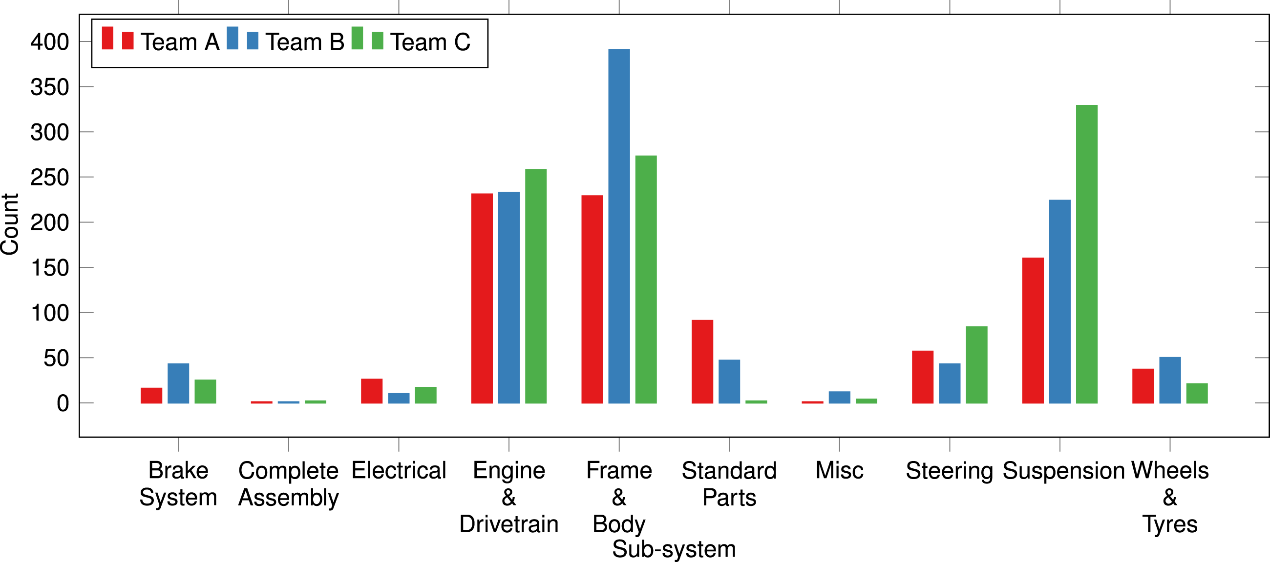
Figure 4. Distribution of product models with respect to the team defined product sub-systems.
Table 5. FS CAD file statistics
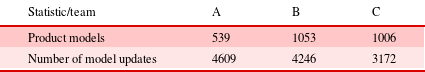
Table 5 presents a summary of the number of files and edits across the three teams. The summary reveals that Teams B and C produced almost twice the number of models compared to that of Team A; however, the total number of edits recorded was consistent between Teams A and B, whilst Team C contained fewer. To further investigate this, Figure 4 shows the distribution of product models by sub-system. This reveals that the additional models present in Teams B and C come from the Frame and Body and Suspension sub-systems, respectively. This aligns with the design intent of the two teams where they have focused on the transient performance and user-centred design aspects of the vehicle and indicates the potential of mapping intent and product performance to structures within the DSM. In all other sub-systems, the number of product models remains fairly consistent across the three teams. The final aspect to note is the reduction in the Standard Part counts across the teams, and following a discussion with the team members, it was revealed that these were allocated to more specific areas of the sub-system architecture. This provides an indication that Teams B and C were more confident in their allocation of the product models during the early design phases than Team A.
5.2 File selection
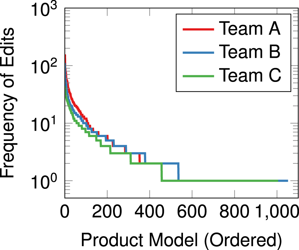
Figure 5. Frequency of edits per product model.
To select the files of interest, Figure 5 shows the frequency distribution of file edits. It is interesting to note that all the teams follow a similar profile with the additional files present within Teams B and C’s datasets appearing to extend the tail of the frequency distribution. This suggests that these files represent standard/bought-in components that are not edited further by the team.
The files are filtered based on the number of updates made. For this study, this has been set to four as this includes the creation of the product model followed by three further updates. This removes models that show little to no activity and may represent constraints in the team’s design space that they are unable to alter (e.g., a bought-in part such as the engine block and/or gearbox) as well as standard parts/fixings (such as nuts and bolts). Following this filtering, the files of interest totalled 353, 379 and 311 for Teams A, B and C, respectively.
5.3 Generation
A time period $(t_{p})$
of 2 h has been selected following the optimisation strategy being performed across the datasets (see Section 5.8). Figure 6 presents the output of this stage, which is an
$(t_{p})$
of 2 h has been selected following the optimisation strategy being performed across the datasets (see Section 5.8). Figure 6 presents the output of this stage, which is an $N\times N$
matrix containing the frequency of co-occurrences between the files.
$N\times N$
matrix containing the frequency of co-occurrences between the files.
Figure 6. Co-occurrence DSMs.
5.4 Normalisation
Following the generation of the co-occurrence DSM, the three teams’ DSMs are normalised. Figure 7 shows the impact of normalisation on the DSMs of the three teams. It is immediately apparent that the normalisation of the co-occurrence of values and distribution of the ratios is consistent across the three teams. This provides an initial indicator that a similar structure is present across the teams.
Figure 7. Conditional probability of file edit co-occurrences.
5.5 Evaluating the ‘directedness’
Table 6 reveals the ‘directedness’ of the teams DSMs with respect to the measure $D$
. In all cases, the measure is significantly low enough to permit the application of an undirected DSM for further partitioning. This was performed on all DSMs for consistency in the analysis.
$D$
. In all cases, the measure is significantly low enough to permit the application of an undirected DSM for further partitioning. This was performed on all DSMs for consistency in the analysis.
Table 6. ‘Directedness’ of the DSMs
5.6 Pruning
The pruning level $(p)$
for the three teams’ datasets was set to 0.3 (see Section 5.8) and the results are presented in Table 7. The pruning has had a considerable effect on reducing the candidate dependencies within the DSMs. The results from the pruning also give an indication to the level of co-occurrence activity with Team A having much greater co-occurrence of activity (40,018) compared to that of Teams B and C. The impact of this is discussed in Sections 6 and 7.
$(p)$
for the three teams’ datasets was set to 0.3 (see Section 5.8) and the results are presented in Table 7. The pruning has had a considerable effect on reducing the candidate dependencies within the DSMs. The results from the pruning also give an indication to the level of co-occurrence activity with Team A having much greater co-occurrence of activity (40,018) compared to that of Teams B and C. The impact of this is discussed in Sections 6 and 7.
Table 7. Reducing the effect of false positive dependencies
5.7 Partitioning
The DSMs are then partitioned and Figure 9 demonstrates the ability for the partitioning technique to reveal the underlying structure in the DSMs. The red boundaries indicate the architecture as planned by the team, whilst the blue boundaries indicate the architecture as designed and produced from this analysis. This visual indication highlights the potential of the technique to uncover the ES within the teams’ architectures. These results, along with the mapping to the hypotheses, form the ES that are presented in the following section.
5.8 Optimisation
To determine $t_{p}$
and
$t_{p}$
and $p$
for the DSM generation, the optimisation strategy was performed across all three datasets and the average for each set of
$p$
for the DSM generation, the optimisation strategy was performed across all three datasets and the average for each set of $t_{p}$
and
$t_{p}$
and $p$
values was taken. Figure 8 shows that a
$p$
values was taken. Figure 8 shows that a $t_{p}=2$
and
$t_{p}=2$
and $p=0.3$
provides the optimum values the three datasets. Also, the variance across the three datasets was very low for the entire range of
$p=0.3$
provides the optimum values the three datasets. Also, the variance across the three datasets was very low for the entire range of $t_{p}$
and
$t_{p}$
and $p$
values, which further highlights the consistency in working practices across the three teams.
$p$
values, which further highlights the consistency in working practices across the three teams.
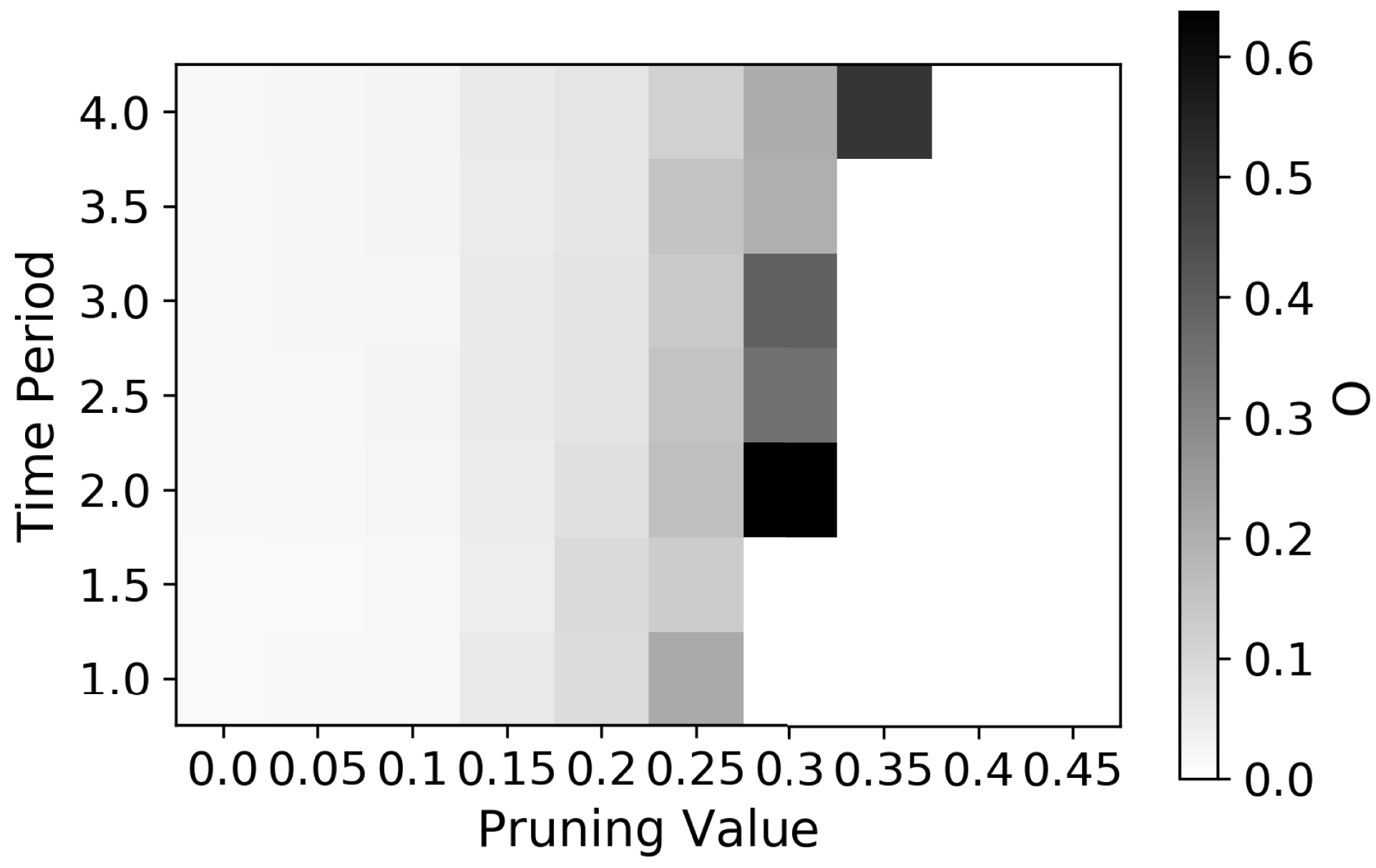
Figure 8. Aggregated optimisation results for the three FS teams.
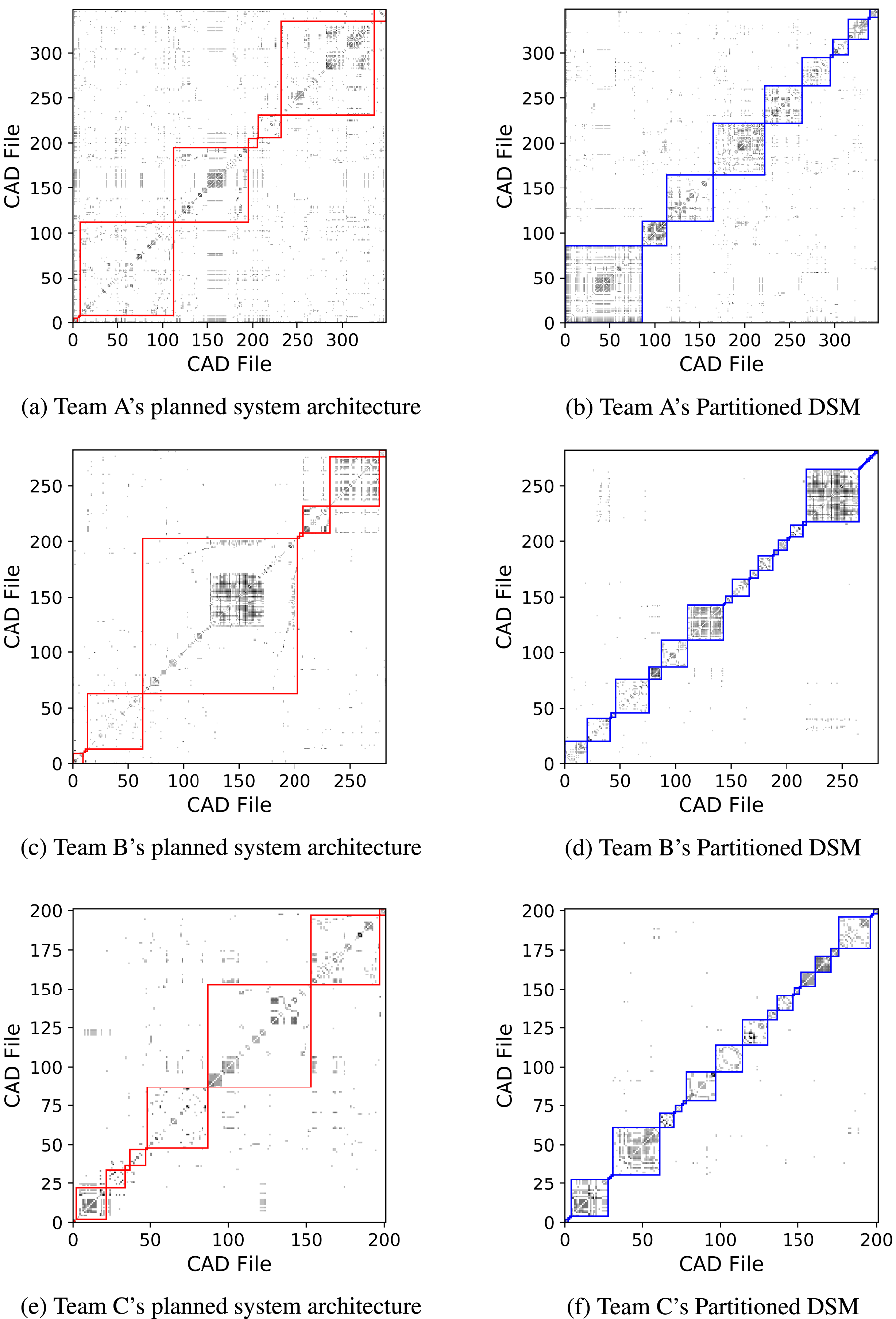
Figure 9. Partitioning of a DSM.
6 Mapping and results
Comparison of the three teams’ DSMs with respect to their design intent and competition performance has been performed through three lenses. These lenses are the comparison of the following:
(1) end-of-project DSM
(2) change propagation characteristics
(3) evolution of the DSMs
The end-of-project comparison examines the final product architecture, whilst the change propagation characteristics reveal the potential impact the product model changes would have across the product architecture. The examination of the evolution of DSMs takes advantage of being able to automatically generate DSMs in real time and examines the working practices among the three teams. This is a feature that has yet to be explored given the lack of datasets to be able to investigate this.
Throughout the presentation of the results, mapping against the teams’ design intent and competition performance has been made. This leads to ES in digital engineering work and is highlighted in the form of $\mathbf{E}\mathbf{S}_{\mathbf{x}}$
. These are subsequently summarised and discussed in Section 7.
$\mathbf{E}\mathbf{S}_{\mathbf{x}}$
. These are subsequently summarised and discussed in Section 7.
6.1 End-of-Project DSMs
Figure 9 and Table 8 present the results from the analysis of the end-of-project DSM. Team A’s DSM has the fewest partitions (9) and components (1) and the lowest modularity (0.56), which reveals that Team A has the most interdependent product model out of the three teams. This is surprising as the team were focusing on an ‘elegant’ design with the aim of keeping it simple. The DSM analysis appears to counter their argument for a simplified design and is a potential reason for them under-performing when compared to Teams B and C.
Table 8. End-of-project DSM summary
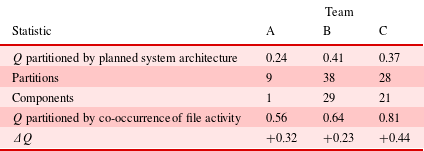
Team B’s design is the most modular with their DSM containing 38 partitions as opposed to 9 and 28 of Teams A and C, respectively. In addition, 29 of these partitions were components. This highlights that Team B had a better understanding of the dependencies between components and were therefore able to generate a more modular design. This is further confirmed by their as-planned partitions scoring a modularity of 0.41, the highest of all the teams. In addition, the team have the smallest $\unicode[STIX]{x1D6E5}Q$
(
$\unicode[STIX]{x1D6E5}Q$
( $+0.23$
) between their as-planned partitioning and the as-designed partitioning, revealing that they had a good understanding of their intended architecture and maintained it through the development and build phases. This is in line with Team B’s design intent of an efficient design process to ensure more testing can be performed.
$+0.23$
) between their as-planned partitioning and the as-designed partitioning, revealing that they had a good understanding of their intended architecture and maintained it through the development and build phases. This is in line with Team B’s design intent of an efficient design process to ensure more testing can be performed.
In contrast, Team C’s DSM has 28 partitions with 21 being components. This shows that Team C’s design consists of fewer, larger modules that are disconnected from one another (Figure 9f). In addition, Team C’s design achieved the highest modularity (0.81) score by partitioning through co-occurrence. This reveals that their as-designed product model is the most structured and well-defined when compared to the other teams, and although you would not expect a modularity score of 1 as interfaces must exist between product models, it highlights that Team C’s interfaces are more defined. In addition, their modularity score increases the most from their as-planned architecture ( $+0.44$
), revealing that they were better at further modularising the architecture during the design phase. This aligns with Team C’s design intent of ‘organisation and planning’ in order to create a well-defined product model. This clarity of interfaces between components is also reflected in their competition performance and indicates a greater knowledge and understanding of their product model. Thus,
$+0.44$
), revealing that they were better at further modularising the architecture during the design phase. This aligns with Team C’s design intent of ‘organisation and planning’ in order to create a well-defined product model. This clarity of interfaces between components is also reflected in their competition performance and indicates a greater knowledge and understanding of their product model. Thus, $\mathbf{E}\mathbf{S}_{\mathbf{1}}$
is that a focus on planning and organisation leads to a more defined product architecture with
$\mathbf{E}\mathbf{S}_{\mathbf{1}}$
is that a focus on planning and organisation leads to a more defined product architecture with $\mathbf{E}\mathbf{S}_{\mathbf{2}}$
showing that a more modular architecture positively affects competition performance.
$\mathbf{E}\mathbf{S}_{\mathbf{2}}$
showing that a more modular architecture positively affects competition performance.
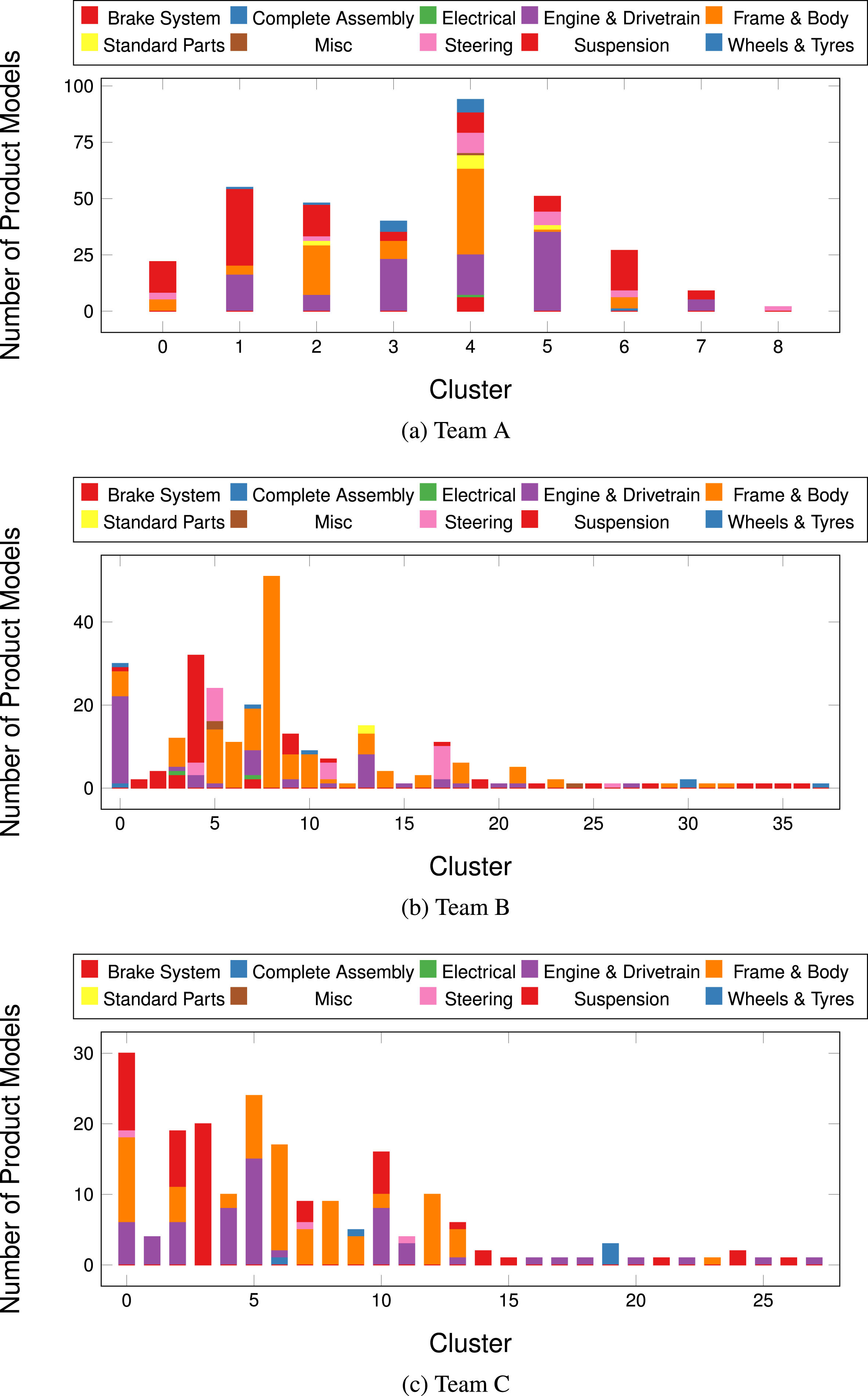
Figure 10. Composition of DSM partitions.
Figure 10 reveals the compositions of the as-designed partitions. Through this, it can be seen that Team A’s partition composition is the most diffuse with each partition featuring a range of product models from the pre-defined sub-systems (Figure 10a). This further highlights that Team A were unable to identify a clear sub-system structure during the early design phases, and this may have led to the issues in the product’s performance and the appropriate allocation of resources during the project.
Figure 10(b) further highlights that Team B’s more modular design can be clearly seen through the greater number of smaller partitions that are focused on single pre-defined sub-systems. In addition, the larger partitions for Team B are noticeably more in line with the initial sub-system classification outlined by the team, which further highlights that Team B were able to better classify the models during the early design phases.
These features are also present in Team C’s composition of clusters (Figure 10b) where there is a number of large inter-related partitions as well as a number of smaller partitions relating to specific sub-systems. These smaller partitions may also relate to specific work packages that were assigned during the generation of the project build. The fact that they exist in the final DSM highlights that Team B and C were both able to identify independent elements of work within the build of the vehicle during the early design phases. This aligns to their design intent of ‘organisation and planning’. Thus, $\mathbf{E}\mathbf{S}_{\mathbf{3}}$
is a clear identification, and adherence to the pre-defined sub-system structure leads to improved competition performance as well as further confirming
$\mathbf{E}\mathbf{S}_{\mathbf{3}}$
is a clear identification, and adherence to the pre-defined sub-system structure leads to improved competition performance as well as further confirming $\mathbf{E}\mathbf{S}_{\mathbf{1}}$
.
$\mathbf{E}\mathbf{S}_{\mathbf{1}}$
.
6.2 Change propagation
A typical application of DSMs is to use them as a predictor/indicator for the capability of a system to accommodate changes along with an evaluation of the level of propagation a change will likely generate (Clarkson, Simons & Eckert Reference Clarkson, Simons and Eckert2004). To investigate this, the study processed the cumulative conditional probabilities of change for each file within the DSM.
This was achieved by taking the file of interest and selecting the files that exist within one and two branch paths. One and two branch paths were selected as the inference of a likely change to a file beyond the third branch has been shown to be unreliable (Pasqual & de Weck Reference Pasqual and de Weck2012). With this list of files and associated one and two branch paths, it is possible to calculate the conditional probability of a change propagating to the neighbouring files.
For example, take File A as the file of interest and File B as a neighbouring file with one and two branch paths between the files. The conditional probability of File B changing is determined by taking the product of probabilities along each of the paths, which gives the probability of each of the paths being traversed, and calculating the probability of at least one of these being traversed if a change occurs. A threshold value for the conditional probability (0.5 in this case) is taken to indicate that a change would occur in B as a result of a change to A.
Table 9. Change propagation statistics
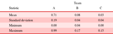
Performing this analysis across all the files gives the distribution of the likely level of change that is to occur across the DSM and gives an insight into the DSMs’ resilience to handle changes. Figure 11 highlights this characteristic through a histogram depicting the proportion of the system that is likely to change by file changes. Table 9 shows the characteristics of each team’s histogram.
Figure 11. Change propagation distribution.
Comparing the distributions, it can be seen that Team A has a much wider distribution over the proportion of system to change with some models requiring checks across almost the entire product architecture. This is in stark contrast to Teams B and C, which exhibit much lower maximum proportions of change values. Inspecting the mean, it can be observed that Team A has a much higher average than that of Team B or C. This indicates that a change within Team A’s product architecture would require significantly more resource in order to handle the propagation of change, thus making it potentially more challenging for the team to accommodate changes. Hence, $\mathbf{E}\mathbf{S}_{\mathbf{4}}$
is that smaller change propagation trees correspond with improved competition performance.
$\mathbf{E}\mathbf{S}_{\mathbf{4}}$
is that smaller change propagation trees correspond with improved competition performance.
Figure 12 shows the distribution of the top 30 product models that are most likely to change as a consequence of a change in another product model. In Team A’s DSM, the top 30 product models are distributed across a range of sub-systems, whilst the most likely models to change from Team B are exclusively from the Frame and Body and Engine and Drivetrain. Team C is similar to that of Team B with the addition of models assigned to the suspension sub-system. As the Frame and Body models form the external structure of the design, this may indicate that Team B’s design was such that any internal changes within the design could be accommodated by the Frame and Body alone. This can also be said for Team C with the suspension sub-system as this is an external element of the vehicle. In contrast, Team A’s design required more extensive cross sub-system alterations to accommodate changes. Therefore, $\mathbf{E}\mathbf{S}_{\mathbf{5}}$
is that competition performance improves when the engineering changes can be accommodated by external sub-systems.
$\mathbf{E}\mathbf{S}_{\mathbf{5}}$
is that competition performance improves when the engineering changes can be accommodated by external sub-systems.

Figure 12. Model most likely to change as a consequence to a change in another model.
6.3 Evolution of DSMs
A particular affordance of automatically generated DSMs is that they can be produced in real time. To investigate this, a pseudo real-time generation of the DSMs for the three projects has been generated. This has been achieved by generating and analysing the DSM as it accumulates product model updates throughout the project. At every product model update, the following characteristics of the DSM have been calculated:
(i) the number of product models that form the DSM;
(ii) the number of dependencies between product models;
(iii) the number of partitions within the DSM;
(iv) the modularity of the DSM;
(v) the number of components within the DSM.

Figure 13. Evolving DSM statistics.
The results are presented in Figure 13 where the cumulation of updates has been normalised in order for comparisons to be made between the three teams. In addition, it can be seen that the lines representing each teams’ DSM do not start at 0 but further along the cumulative update scale. This is due to the fact that during this period, the number of co-occurrences is insufficient to form a DSM.
Looking at the number of product models within the DSM (Figure 13a), it is interesting to note the similarity in the generation of models over the course of each project. This indicates that there is a relationship between the number of updates and maturity of the product architecture. This result provides evidence for $\mathbf{E}\mathbf{S}_{\mathbf{6}}$
, which states that normal and predictable behaviours exist in the design process of near-identical projects.
$\mathbf{E}\mathbf{S}_{\mathbf{6}}$
, which states that normal and predictable behaviours exist in the design process of near-identical projects.
However, differences start to appear when one focuses on the number of co-occurrences weighted ${>}0.25$
(Figure 13b). Co-occurrences appear early and see considerable growth for Teams A and B, whilst Team C’s co-occurrences ramp up more gradually and plateaus. Both Teams A and B see a continuing rise with an abrupt change in the number of co-occurrences near the end of the project, which indicates a significant change in product architecture and potential rush to finish the product model before the deadline. With Team C performing the best out of the three teams,
${>}0.25$
(Figure 13b). Co-occurrences appear early and see considerable growth for Teams A and B, whilst Team C’s co-occurrences ramp up more gradually and plateaus. Both Teams A and B see a continuing rise with an abrupt change in the number of co-occurrences near the end of the project, which indicates a significant change in product architecture and potential rush to finish the product model before the deadline. With Team C performing the best out of the three teams, $\mathbf{E}\mathbf{S}_{\mathbf{7}}$
is that gradual and steady growth of co-occurrences between product models has a positive relation to competition performance.
$\mathbf{E}\mathbf{S}_{\mathbf{7}}$
is that gradual and steady growth of co-occurrences between product models has a positive relation to competition performance.
Figure 13(c) reveals the number of partitions identified with an almost linear relationship between partitions and cumulative updates being exhibited. This suggests that if the design begins with a high number of partitions, then the product architecture will continue to be highly partitioned. In addition, the lines appear rather jagged, showing the continual addition, merging and parting of partitions within the DSMs as they evolve. Thus, $\mathbf{E}\mathbf{S}_{\mathbf{8}}$
is that a modular architecture at the start of the design process will promote further modularisation of the product architecture.
$\mathbf{E}\mathbf{S}_{\mathbf{8}}$
is that a modular architecture at the start of the design process will promote further modularisation of the product architecture.
Figure 13(d) reveals how the modularity of the DSM evolves throughout the cumulation of updates. Modularity indicates the level of structure that resides within the matrix with a score of ${>}0.25$
indicating a structure that is beyond random chance. In the case of the three teams, it can be seen that the values calculated are consistently higher than pure chance and, thus, provides further evidence that the method is capturing and providing design process insights. Overall, all teams’ modularity scores increase as the updates accumulate with Team C achieving the highest modularity score. Thus,
${>}0.25$
indicating a structure that is beyond random chance. In the case of the three teams, it can be seen that the values calculated are consistently higher than pure chance and, thus, provides further evidence that the method is capturing and providing design process insights. Overall, all teams’ modularity scores increase as the updates accumulate with Team C achieving the highest modularity score. Thus, $\mathbf{E}\mathbf{S}_{\mathbf{9}}$
is that the design process can be described as a process of continually increasing the level of structure between a set of product models.
$\mathbf{E}\mathbf{S}_{\mathbf{9}}$
is that the design process can be described as a process of continually increasing the level of structure between a set of product models.
In addition, Team C provides an interesting feature within Figure 13(d) where there is a significant decrease in modularity before returning to its previous value. Upon reviewing the design reports of the team, it was discovered that each sub-team developed their assemblies away from one another before integrating them to form the complete assembly model. The feature within Figure 13(d) aligns with this event.
The final aspect monitors the number of components throughout the evolution of the DSM (Figure 13e). This follows a similar trend to that of the partitions within the DSM where Teams B and C see a continual growth in the number of components, whilst Team A contains very few. This highlights the potential increase in the modular architecture of Teams B and C compared with Team A. In addition, Teams B and C both have a sudden increase in the number of components as they move beyond 0.8 cumulative updates. As these are components and not partitions, this suggests that these product features are separate to the main product architecture. Interrogation of the product models within these components highlighted that these were finishing touches to the product such as the decals on the bodywork and ancillary elements to the aero package (e.g. gurney flap). It is interesting to see that Team A were unable to reach this part of the design process and may relate to the relative lack of performance in the competition as their product had not reached the maturity of Teams B and C. Therefore, $\mathbf{E}\mathbf{S}_{\mathbf{10}}$
is that the final stages of an FS design process are indicated by a sudden increase in the number of components to the DSM.
$\mathbf{E}\mathbf{S}_{\mathbf{10}}$
is that the final stages of an FS design process are indicated by a sudden increase in the number of components to the DSM.
7 Discussion and future work
The results and mapping to the design intent and competition performance have identified 10 ES that could be used as references to support the management of future FS projects. The 10 ES are as follows:
-
$\mathbf{E}\mathbf{S}_{\mathbf{1}}$
A focus on planning and organisation leads to a more defined product architecture.
-
$\mathbf{E}\mathbf{S}_{\mathbf{2}}$
A more modular architecture positively affects competition performance.
-
$\mathbf{E}\mathbf{S}_{\mathbf{3}}$
A clear identification and adherence to the pre-defined sub-system structure leads to improved competition performance.
-
$\mathbf{E}\mathbf{S}_{\mathbf{4}}$
Smaller change propagation trees correspond with improved competition performance.
-
$\mathbf{E}\mathbf{S}_{\mathbf{5}}$
competition performance improves when the engineering changes can be accommodated by external sub-systems.
-
$\mathbf{E}\mathbf{S}_{\mathbf{6}}$
Normal and predictable behaviours exist in the design process of near-identical projects.
-
$\mathbf{E}\mathbf{S}_{\mathbf{7}}$
Gradual and steady growth of co-occurrences between product models has a positive relation to competition performance.
-
$\mathbf{E}\mathbf{S}_{\mathbf{8}}$
A modular architecture at the start of the design process will promote further modularisation of the product architecture.
-
$\mathbf{E}\mathbf{S}_{\mathbf{9}}$
The design process can be described as a process of continually increasing the level of structure between a set of product models.
-
$\mathbf{E}\mathbf{S}_{\mathbf{10}}$
The final stages of an FS design process are indicated by a sudden increase in the number of components to the DSM that relates to ‘finishing touches’.


Upon reflection of the ES and the processing used to generate them, it is contended that the analysis of the end-of-project DSMs and change propagation statistics lend themselves to the generation of insights on the products’ design. However, the analysis of the evolution of DSMs tends to produce insights that concern the design process.
Although this study has demonstrated the elicitation of ES from the mapping of design intent and competition performance to the analysis of DSMs, the elicitation process remains highly qualitative and subjective due to the interpretation of the design researchers. To improve the accuracy of the interpretations, further work could be performed in developing methodologies of capturing design intent throughout the design process. Such tools include work activity monitoring tools developed by Robinson (Reference Robinson2012) and Škec, Cash & Štorga (Reference Škec, Cash and Štorga2017).
To confirm these ES, the authors are currently capturing further FS projects that will enable them to statistically model and provide relationships between DSMs and design intent/competition performance with greater confidence and significance. Upon completion of this exercise, the authors wish to investigate how the introduction of dynamic DSMs and insights can support project management activities.
In addition, there is a need to expand the analysis to other engineering projects where it has been contended that the analysis would be more suitable for large multi-disciplinary and distributed projects where managers are unable to maintain direct dialogues with all the engineers involved. Although, the analysis is capable of being performed on any engineering projects’ digital footprint, further studies need to be performed to confirm which types of project benefit the most from the insights that the analysis can draw.
Nonetheless, this study has realised the potential of the engineering digital footprint to provide ES. ES can now be monitored in real time in new projects through the continual analysis of their evolving digital footprints. The information provided back to the design team and managers can now enable a more pro-active approach to the engineering project management and is an area that the authors are currently investigating.
8 Conclusion
DSMs have become a fundamental tool to support engineers in their handling and management of interactions across product and organisational architectures. With the advent of the ever-increasing engineering digital footprint, methods now exist to generate DSMs continuously and in real time through the co-occurrence of edits to engineering files. This ability to systematically generate DSMs throughout an engineering project now provides researchers with a more objective method of viewing the evolution of a project and enables cross-project comparisons to occur.
This paper has exploited this potential by being the first to compare dynamic DSMs for three near-identical system design projects. Through comparison of the end-of-project DSMs and change propagation characteristics of the DSMs, 10 ES have been elicited. These ES are considered in the context of team performance and the design intents of the three teams in order to explain the identified structures. The 10 structures are found to relate to approaches for organisation and management, level of consideration of modularity and levels of performance (quality and time). It is further shown how these 10 structures can be utilised by engineers to improve the management of future system design projects. A key affordance of this approach is the ability to monitor them in real time through the analysis of DSMs, thereby leading to more pro-active project management strategies.
Acknowledgments
The work reported in this paper has been undertaken as part of the EPSRC Language of Collaborative Manufacturing (EP/K014196/2), UKRI NCC Researcher in Residence (EP/R513556/1) and EPSRC Trans-disciplinary Engineering (EP/R013179/1) Grants held at the University of Bath and University of Bristol. Underlying data are openly available from the University of Bath Research Data Archive at https://doi.org/10.15125/BATH-00621.


 Open access