

1. Introduction
Survival analysis entails analysing data on the length of time until occurrence of an event, such as the time to death (Therneau & Grambsch, Reference Therneau and Grambsch2000). A survival model is a regression model fitted on the data and estimates the time to an event based on several risk factors, such as sociodemographic factors, lifestyle factors, medical conditions, and medical interventions (Therneau & Grambsch, Reference Therneau and Grambsch2000). This type of research is typically done in the medical field. Survival models are of interest to clinicians, because they can identify specific patient characteristics associated with different survival rates. These findings can be used to counteract the harmful effects and enhance the protective effects of modifiable risk factors, for example, blood pressure could be targeted to improve survival prospects.
Survival models could also be of interest in retirement planning, life and health insurance, and pensions. The key information in retirement planning is life expectancy at the individual and population levels. Current life expectancy and future projections can inform individuals about how to spend their pension pot during retirement, inform actuaries about pricing of annuities and life insurance, and inform governments about taxation, national insurance rates, and pensions.
At an individual level, survival models that allow for differences in risk factors enable estimates of life expectancy to be tailored for that individual rather than assuming an aggregate population figure. This can help that individual with retirement planning, or help an underwriter to offer the appropriate rate for an enhanced annuity. Indeed, “effective ages” are often used by insurers as a way of applying the correct rating to an underwritten life.
Insurers, pensions providers and others are often interested in projecting life expectancies for a sub-population that is different from the population as a whole, for example, by socioeconomic group or, for an underwritten sub-population, by health status. This can lead to basis risk which can be reduced by using survival models that allow for factors that differ between the sub-population and the population. The examples below describe this in terms of two medical interventions. Gitsels et al. (Reference Gitsels, Kulinskaya and Steel2017) present models that also allow for socioeconomic differences in the prevalence of treatments via Mosaic categories. Applying the methods described in this paper can help to understand the extent that differences in mortality improvements between a population and a sub-population can be explained by differences in anti-hypertensive drug prescription, for example, and to project improvements with more confidence.
Changes in life expectancies can be calculated from the survival models estimated hazard ratios of all-cause mortality. The tools needed for this calculation are a survival model, information on the prevalence of the risk factor of interest, and a life table.
First, we provide some background on Cox’s proportional hazards survival models and the meaning of a hazard ratio. Next, we show how estimated hazards of mortality associated with risk factors can be translated to changes in life expectancies at the individual and population levels using an “effective age” and period life expectancies. This will be illustrated by two examples of medical interventions and their associated impact on life expectancy: beta blockers, a type of blood pressure treatment, in heart attack survivors, and overall blood pressure treatment in hypertensive patients. Using data from a UK primary care database, the survival models are estimated at different retirement ages. The estimated hazard ratios are translated to changes in life expectancies at the individual and population levels for men and women at ages 60, 65, 70, and 75 in the United Kingdom.
2. Hazard Ratio
The type of regression model typically used in survival analysis in medicine is the Cox’s proportional hazards regression model (Therneau & Grambsch, Reference Therneau and Grambsch2000). The “hazard of mortality” is also commonly referred to as “force of mortality” and “mortality intensity”.
The Cox’s model estimates the hazard μ i (x) for subject i at time x by multiplying the baseline hazard function μ 0(x) by the subject’s risk score r i (Therneau & Grambsch, Reference Therneau and Grambsch2000):
 $$\mu _{i} \left( {x,\beta ,Z_{i} } \right){\equals}\mu _{0} \left( x \right)r_{i} \left( {\beta ,Z_{i} } \right){\equals}\mu _{0} \left( x \right)e^{{\beta {\rm }Z_{i} }} {\rm }$$
The risk score is dependent of the values of the multiple risk factors Z and their coefficients β. Taking a ratio of the hazard functions for two subjects i and j who differ in one risk factor z and not in the other risk factors, the coefficient β
z
or the hazard ratio $e^{{\beta _{z} }} $
per unit increase of risk factor z can be calculated (Therneau & Grambsch, Reference Therneau and Grambsch2000):
$e^{{\beta _{z} }} $
per unit increase of risk factor z can be calculated (Therneau & Grambsch, Reference Therneau and Grambsch2000):
 $$\mu \left( {x,\beta ,Z} \right){\equals}{\rm }{{\mu _{i} \left( {x,{\rm }\beta ,{\rm }Z_{i} } \right)} \over {\mu _{j} \left( {x,{\rm }\beta ,{\rm }Z_{j} } \right)}}{\equals}{{\mu _{0} \left( x \right)e^{{\beta {\rm }Z_{1} }} } \over {\mu _{0} \left( x \right)e^{{\beta {\rm }Z_{0} }} }}{\equals}{\rm }{{e^{{\beta _{z} {\rm }z_{1} }} } \over {e^{{\beta _{z} {\rm }z_{0} }} }}{\equals}e^{{\beta _{z} {\rm }(z_{0} {\minus}z_{1} )}} $$
This means that the baseline hazard μ
0(x) does not have to be specified and the hazard ratio $e^{{\beta _{z} }} $
is constant with respect to time x. In other words, the Cox’s model does not make any assumptions about the shape of the baseline hazard function, but does assume proportional hazards for the risk factors over time x. The time x may be age, or the time from the study entry. The assessment of the proportional hazards assumption can be done visually by, for example, Kaplan–Meier plots or numerically by, for example, the Grambsch and Therneau’s test (Therneau & Grambsch, Reference Therneau and Grambsch2000). This test statistic can be interpreted as a measure of the correlation between the residuals from the model and event times. If the proportional hazards assumption is violated, the risk factor should be specified differently by, for example, specifying time-dependent effects where follow-up time is split in intervals in which the proportional hazards assumption holds.
$e^{{\beta _{z} }} $
is constant with respect to time x. In other words, the Cox’s model does not make any assumptions about the shape of the baseline hazard function, but does assume proportional hazards for the risk factors over time x. The time x may be age, or the time from the study entry. The assessment of the proportional hazards assumption can be done visually by, for example, Kaplan–Meier plots or numerically by, for example, the Grambsch and Therneau’s test (Therneau & Grambsch, Reference Therneau and Grambsch2000). This test statistic can be interpreted as a measure of the correlation between the residuals from the model and event times. If the proportional hazards assumption is violated, the risk factor should be specified differently by, for example, specifying time-dependent effects where follow-up time is split in intervals in which the proportional hazards assumption holds.
An adjusted hazard ratio of mortality is interpreted as the instantaneous increased or decreased hazard of mortality associated with a unit change from the reference value of the risk factor adjusted for the other risk factors averaged over the length of the study period. In case of a binary risk factor where absence is the reference value, then a hazard ratio <1 (i.e. a negative estimated coefficient $ \widehat{{\beta _{z} }}$
) means that the presence of the risk factor is associated with a decreased hazard of mortality and a longer survival time. Similarly, a hazard ratio >1 (i.e. a positive estimated coefficient
$ \widehat{{\beta _{z} }}$
) means that the presence of the risk factor is associated with a decreased hazard of mortality and a longer survival time. Similarly, a hazard ratio >1 (i.e. a positive estimated coefficient $ \widehat{{\beta _{z} }}$
) means that the presence of the risk factor is associated with an increased hazard of mortality and a shorter survival time.
$ \widehat{{\beta _{z} }}$
) means that the presence of the risk factor is associated with an increased hazard of mortality and a shorter survival time.
3. Effective Age
A hazard ratio of mortality is a relative term indicating how much better or worse off a person with a risk factor is compared to a person without the risk factor with respect to their instantaneous hazard of death. This relative term can be difficult to comprehend. In some contexts, in medicine as well as in insurance, a probability of seeing a certain event in some group is called risk, while the term incidence is used in epidemiology. Hence, the risk ratio, or relative risk, often is the effect measure of choice. Since the hazard ratio is also a relative measure, sometimes it is mistakenly interpreted as relative risk. However, the hazard ratio is the ratio of the forces of mortality at a time x, whereas the relative risk is the ratio of the probabilities of death over an interval from 0 to x.
To facilitate the understanding of the hazard ratio, in recent years medical research has presented hazards also as the difference in the chronological age and the “effective age”, which is the average age with the same hazard (Spiegelhalter, Reference Spiegelhalter2016). This difference in ages indicates “premature ageing” if the effective age is higher than the chronological age or “rejuvenation” if the effective age is lower than the chronological age, see Figure 1.
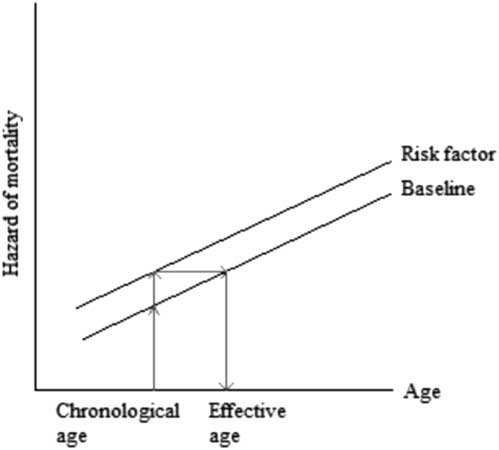
Figure 1 Translating hazard of mortality to change in age
The difference between the chronological and effective ages can also be expressed as the number of years gained or lost in age due to the unit change in risk factor. For simplicity, consider a binary risk factor where absence is the reference value (z=0) and presence is the unit change (z=1). The translation from a hazard of mortality to the number of years gained or lost in age is based on the condition that there are proportional hazards as assumed by the Cox’s model and the condition that the baseline hazard rate of a population increases linearly with age x on the log scale (Spiegelhalter, Reference Spiegelhalter2016). These conditions can be expressed as the hazard of mortality μ(x) being equal to the hazard associated with the risk factor e βz and the hazard associated with ageing e α+ γx , μ(x)=e βz +α+ γx . That is, the baseline Gompertz’ survival distribution is assumed for this calculation. Then, the number of years gained or lost in age x is the log of hazard ratio e β divided by the log of increase in annual hazard rate in a population e γ , Δx=β/γ.
As showed by Gompertz’ model applied to numerous populations over time, the rate of increase e γ in the hazard of mortality associated with ageing 1 year is approximately constant between the ages of 50 and 95 (Brenner et al., Reference Brenner, Gefeller and Greenland1993; Vaupel, Reference Vaupel2010; Spiegelhalter, Reference Spiegelhalter2016), our target ages for retirement. In this paper, we consulted the life table of 2010 of the United Kingdom to calculate the annual rate of increase e γ in the hazard of mortality in the UK population (Office for National Statistics, 2017). The life tables are based on the population estimates and deaths by date of registration data for a period of 3 consecutive years. The annual rate of increase e γ for men and women between the ages 50 and 95 was approximately 1.107 and 1.115, respectively (Figure 2). Subsequently, Δx number of years gained or lost in age due to the presence of risk factor z is:
 $$\Delta x{\equals}{{\log (e^{{{\rm \beta }_{z} {\rm }}} )} \over {{\rm log}(e^{\gamma } )}}\,\approx\,{{\beta _{z} } \over {{\rm log}(1.107)}}\rm \,for\;men,\,and$$
 $$\Delta x{\equals}{{\log (e^{{{\rm \beta }_{z} {\rm }}} )} \over {{\rm log}(e^{\gamma } )}}\,\approx\,{{\beta _{z} } \over {{\rm log}(1.115)}}\, \rm for\;women.$$
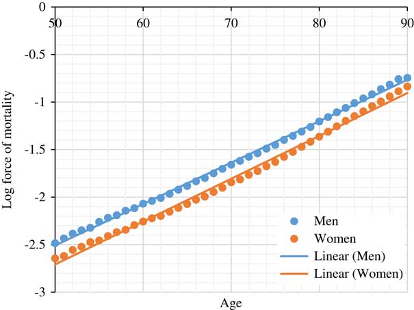
Figure 2 Log force of mortality for UK population based on 2010 period life table (Office for National Statistics, 2017)
This translation from hazard ratio to effective age could be used to explain to individuals the consequences of various diseases and lifestyle choices and as a result persuade clients in life and health insurance to pursue a healthier lifestyle.
4. Period Life Expectancy
The period life table presents the period life expectation (LE) e x at age x, which is the weighted average of the period life expectancies of people with different risk profiles at age x. Let e x,1 and e x,0 be the period life expectancies for people with and without the risk factor (reference subpopulation), respectively, at age x. Then, the period life expectancy of the overall population e x at age x with its prevalence of the risk factor p x at age x is defined as
 $$e_{x} {\equals}p_{x} e_{{x,1}} {\plus}\left( {1{\minus}p_{x} } \right)e_{{x,0}} .$$
Changes in the prevalence of the risk factor p x would result in changes in the period life expectancy of the population e x at age x, ranging from e x,0 in the complete absence of the risk factor to e x,1 in the complete presence of the risk factor.
When the proportional hazards assumption is satisfied, the overall (known) period LE e x can be easily decomposed into the constituent LEs e x,1 and e x,0, which have known weights defined by prevalences. On the log-hazard scale, the constituent log forces of mortality can be drawn as parallel curves which differ in intercepts defined by one or more known parameters (the log-hazard ratios of the risk factors and/or interventions). The shape of these curves is defined by the baseline hazard function μ 0 (x). Figures 4 and 5 depict these shapes for heart attack survivors and hypertensive patients. The baseline log-hazard is simply a straight line if the Gompertz’ survival distribution provides a good fit. In this case, the only unknown parameter is the intercept for the reference log-hazard rate, which can be derived from the equation (1). See Ashwell et al. (Reference Ashwell, Mayhew, Richardson and Rickayzen2014) and Li (Reference Li, Hüsing and Kaaks2014) for similar derivations on the impact of obesity and other lifestyle risk factors on life expectancy assuming the Gompertz distribution.
In the following two sections, examples are given that illustrate how the hazard of mortality associated with a risk factor is estimated in a sample of a population and how the estimated hazard of mortality is translated to changes in life expectancies at the individual and population levels. The implicit assumption of these calculations is that the shape of the baseline hazards (and therefore of the survival functions generated by the survival model) in the sample of the population is the same as that of in the full population of interest (which can be obtained from national period life tables if the entire population is of interest). This assumption is vital for the generalisability of the results of clinical studies to the underlying population.
5. Example on Treatment in Heart Attack Survivors
In a previous study, we estimated the hazard of mortality associated with a history of heart attack in UK residents and how the survival prospects were changed by first line treatments of heart attack (Gitsels et al., Reference Gitsels, Kulinskaya and Steel2017). In this example, we focus on the results on the recommended prescription of beta blockers, which is a type of blood pressure treatment (National Institute for Clinical Excellence, 2013), in heart attack survivors, and translate these results to changes in life expectancies of heart attack survivors at the individual and population levels. Coronary heart disease is the UK’s single biggest killer, of which most deaths are caused by heart attack (British Heart Foundation, 2016). In the United Kingdom, about seven out of 10 people survive a heart attack, resulting in almost two million UK residents having survived a heart attack (Townsend et al., Reference Townsend, Williams, Bhatnagar, Wickramasinghe and Rayner2014).
In our study on heart attack (Gitsels et al., Reference Gitsels, Kulinskaya and Steel2017), we selected data from The Health Improvement Network (THIN) UK primary care database. This is a primary care database, which medical records are representative of the UK population when adjusted for sex, age and deprivation (Hall, Reference Hall2009; Blak et al., Reference Blak, Thompson, Dattani and Bourke2011). The study design was a matched retrospective cohort study, where each patient with a history of heart attack was matched to three controls on sex, year of birth, and clinic. We selected four cohorts of patients who reached the target age between 1987 and 2011 and were followed-up to 2011. The target ages were 60, 65, 70, and 75, and their respective cohorts included 16,744, 43,528, 73,728, and 76,392 patients. The risk factor of interest was the prescription of beta blockers, which across the target ages was prescribed in 44%–48% of the heart attack survivors. The outcome of interest was time to death from any cause, which across the target ages was observed in 22%–24% of the heart attack survivors who were prescribed beta blockers and in 33%–37% of the heart attack survivors who were not prescribed the drugs. See Figure 3 for details of the data selection.
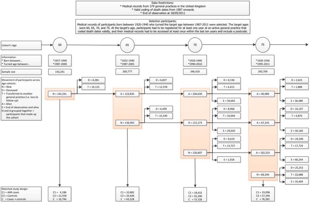
Figure 3 Data selection for the heart attack study. Reproduced from Gitsels et al. (Reference Gitsels, Kulinskaya and Steel2017)
We estimated the hazard of all-cause mortality associated with the prescription of beta blockers by a Cox’s proportional hazards regression and adjusted for sex, year of birth, deprivation, several heart conditions including heart attack, chronic kidney disease, diabetes, high blood pressure, high cholesterol level, heart surgery, prescription of “first line” drugs to treat a heart attack, body mass index, alcohol consumer status, smoking status, and clinic. All measurements were taken at the baseline target age. We fitted this survival model for each age cohort. The proportional hazards assumption was assessed by Therneau & Grambsch’s test (Reference Therneau and Grambsch2000) and indicated no violations.
Compared to no history of heart attack, a history of one heart attack by age 60, 65, 70, or 75 was associated with an increased hazard of mortality of 1.80 (95% confidence interval of 1.60–2.02), 1.71 (1.59–1.84), 1.50 (1.42–1.59), or 1.45 (1.38–1.53), respectively. In heart attack survivors, compared to no prescription of beta blockers, a prescription of beta blockers by age 60, 65, 70, or 75 was associated with a decreased hazard of mortality of 0.83 (0.73–0.94), 0.79 (0.73–0.85), 0.85 (0.81–0.91), and 0.81 (0.77–0.86), respectively. In patients who did not have a history of heart attack, prescription of beta blockers was not associated with a change in survival prospects. There were no interaction effects between history of heart attack and sex or between prescription of beta blockers and sex, indicating that the respective survival prospects were the same for men and women.
The hazard of mortality associated with a history of one heart attack by the target ages translated to 3.7–5.8 years gain in age (i.e. “ageing”) for a man and 3.4–5.4 years gain in age for a woman. This is the change from the chronological to the effective age for a heart attack survivor. The hazard of mortality associated with a prescription of beta blockers to a heart attack survivor by the target ages translated to 1.6–2.3 years decrease in age (“rejuvenation”) for a man and 1.5–2.2 years decrease in age for a woman. The change from the chronological to the effective age in a heart attack survivor who is prescribed beta blockers is the sum of the number of years gained by a history of heart attack and by a prescription of beta blockers. This means that a male or female heart attack survivor who is prescribed beta blockers gained 1.6–3.9 years in age or 1.5–3.7 years in age, respectively.
The log forces of mortality were derived from the fitted Cox’s proportional hazards regression that was fully adjusted by the factors listed above. The baseline hazard rate (i.e. force of mortality in the reference group) was derived from the cumulative baseline hazard rate estimated by the model. Then, the baseline hazard rate was multiplied by the estimated hazard ratio of the risk factor of interest, here heart attack, resulting in the force of mortality in heart attack survivors. Next, this hazard rate was multiplied by the estimated hazard ratio of the intervention of interest, here beta blockers, resulting in the force of mortality in heart attack survivors who were prescribed beta blockers. Figure 4 depicts the log forces of mortality for the four age cohorts, men and women separately. These are parallel curves that are approximately straight lines for ages 65 years and older. These curves differ in intercepts defined by the log-hazard ratios of the heart attack and of treatment by beta-blockers in heart attack survivors, and by the intercept of the baseline risk curve. The shape of these curves is defined by the baseline hazard function μ 0(x) (black line).

Figure 4 Log force of mortality in non-heart attack survivors (black), heart attack survivors (blue), and heart attack survivors on beta blockers (green) by sex and age. Log force of mortality adjusted for year of birth (reference of 1931–1935), deprivation (reference of “Alpha territory” by Mosaic), lifestyle factors (reference of healthy), and medical history (reference of healthy).
The overall period life expectancy of heart attack survivors can be calculated using the prevalence of heart attack, the requisite hazard ratios, and the overall period life expectancy in the general population. In the next step, the period life expectancies of heart attack survivors not prescribed beta blockers and those prescribed beta blockers can be calculated using the prevalence of prescription of beta blockers in heart attack survivors (Table 1), the requisite hazard ratios and the overall period life expectancy of heart attack survivors (obtained from the previous step). Table 2 presents these calculated period life expectancies at chronological ages 60, 65, 70 and 75 by sex.
Table 1 Prescription Level of Beta Blockers in Heart Attack Survivors in the Age Cohorts

Author’s computations.
Table 2 Period Life Expectancy for Heart Attack Survivors at 2010 Prescription Level of Beta Blockers and Period Life Expectancies for Heart Attack Survivors With or Without Prescription of Beta Blockers
The period life expectancies (95% confidence intervals (CI)) are based on the UK life table centred 2009–2011 (Office for National Statistics, 2017).
* Period life expectancy for heart attack survivors at 2010 prescription level of beta blockers. This period life expectancy is the weighted average of the next two period life expectancies:
† Period life expectancy for heart attack survivors with prescription.
‡ Period life expectancy for heart attack survivors without prescription.
Hypothetical changes in the overall life expectancy of heart attack survivors can be derived from changes in the prevalence of prescription of beta blockers in this group. For example, if all men surviving a heart attack by age 60 would be prescribed beta blockers, then their population life expectancy would increase from 17.4 to 18.8 years, while if all would not be prescribed the drugs, their population life expectancy would decrease to 16.4 years. Similarly, for women surviving a heart attack by age 60, if all would be prescribed beta blockers, their population life expectancy would increase from 20.3 to 21.8 years, while if all would not be prescribed the drugs, their population life expectancy would decrease to 19.3 years.
6. Example on Treatment in People with High Blood Pressure
This example is about blood pressure treatment given to people with hypertension. A comparative risk assessment of burden of disease and injury showed that high blood pressure is the number one risk factor of global disease burden (Gakidou et al., Reference Gakidou, Afshin, Abajobir, Abate, Abbafati, Abbas, Abd-Allah, Abdulle, Abera, Aboyans and Abu-Raddad2017). The prevalence of high blood pressure, defined as a systolic blood pressure of 140 mmHg or higher, is 32% in the United States and 30% in the United Kingdom (British Heart Foundation, 2016; Whelton et al., Reference Whelton2017).
An influential US clinical trial named SPRINT examined the effect of lowering systolic blood pressure to less than 120 mmHg (intensive treatment) instead of to less than 140 mmHg (standard treatment) in patients with high blood pressure (SPRINT Research Group, 2015). The trial included 9,361 hypertensive patients aged 50–90 and had a median follow-up of 3.3 years. Half of the patients were assigned the intensive treatment of blood pressure of whom 3.3% died from any cause during the follow-up. In the standard treatment arm, death was observed in 4.5% of the patients. Compared to the standard treatment of blood pressure, the intensive treatment was associated with a decreased hazard of all-cause mortality of 0.73 (95% confidence interval of 0.60–0.90) (SPRINT Research Group, 2015). The annual mortality rate for men and women at ages 50–95 in the United States in 2010 was approximately 1.092 and 1.098, respectively (Social Security Administration, 2014). This means that the intensive treatment of high blood pressure translated to the number of years lost in age (“rejuvenation”) of 3.6 years in men and 3.4 years in women.
Recent evaluation of the research evidence on blood pressure thresholds for intervention by the American Heart Association (AHA) (Whelton et al., Reference Whelton2017) and the Scottish Intercollegiate Guidelines Network (SIGN, 2017) led to different updated hypertension guidelines. While the AHA changed its hypertension guideline on the basis of SPRINT results (Whelton et al., Reference Whelton2017), the SIGN did not because the trial was not regarded to be generalisable to the routine clinical practice in Scotland mainly due to how blood pressure was measured (SIGN, 2017). Other reasons why the results might not be generalisable to the general population are the trial’s restricted inclusion criteria of patients and the trial’s short follow-up of patients. The question remains what the optimal blood pressure is in people treated for hypertension in routine clinical practice. For this reason, we estimated the long-term survival prospects associated with the intensive treatment of blood pressure in hypertensive patients who were seen in primary care in the United Kingdom (Gitsels et al., 2018).
We selected data of THIN database. The study design was a retrospective cohort study. The sample included 54,683 patients who were treated for hypertension between 2005 and 2013 and followed-up to 2017. Patients had their systolic blood pressure dropped from more than 140 mmHg (baseline) to between 121 and 140 mmHg (standard treatment) or to 120 mmHg or less (intensive treatment). At baseline, patients were between 50 and 90 years old. The risk factor of interest was intensive treatment of blood pressure, which was observed in 36% of the patients. The outcome of interest was time to death from any cause, which was observed in 13% of the patients on the intensive treatment and 11% of the patients on the standard treatment. See Table 3 for details.
Table 3 Characteristics of The Health Improvement Network (THIN) Cohort of Hypertensive Patients

Standard treatment of lowering systolic blood pressure to ≤140 mmHg and intensive treatment of lowering systolic blood pressure to ≤120 mmHg.
We estimated the hazard of all-cause mortality associated with the intensive treatment of blood pressure by a Cox’s proportional hazards regression and adjusted for the number of anti-hypertensive drugs prescribed at the baseline, the change in the number of anti-hypertensive drugs prescribed at the dropped blood pressure measurement, prescription of several other drugs at baseline, history of cardiovascular disease at baseline, sex, age at baseline, deprivation at baseline, smoking status at baseline, and clinic. The proportional hazards assumption was assessed by Therneau & Grambsch’s test (Reference Therneau and Grambsch2000) and the effect of a violated risk factor was made time-dependent.
Compared to the standard blood pressure treatment, the intensive treatment was associated with an increased hazard of mortality of 1.21 (95% confidence interval of 1.15–1.27). Thus, the intensive treatment appears to be harmful, contradicting the SPRINT findings. There were no interaction effects between blood pressure treatment and sex or age, indicating that the effect of intensive treatment associated with the hazard of mortality was the same for men and women and across ages.
As the studied cohort included only hypertensive patients, the hazard of mortality associated with hypertension could not be estimated. This hazard is needed to calculate the overall period life expectancy of people with hypertension and the resulting period life expectancies of people on intensive blood pressure treatment and of people on standard blood pressure treatment. Therefore, we additionally selected four cohorts who reached the target age between 1987 and 2011 and were followed-up to 2011. The target ages were 60, 65, 70, and 75, and each age cohort included between 140,000 and 350,000 patients. The selection of the target age cohorts was similar to that for the heart attack study given in Figure 3, and was not the matched study design as with the heart attack study. The risk factor of interest was hypertension, which across the target ages was observed in 63%–76% of the patients. The outcome of interest was time to death from any cause, which across the target ages was observed in 16%–21% of the hypertensive patients and in 12%–19% of the normotensive patients. We estimated the hazard of all-cause mortality associated with hypertension by a Cox’s proportional hazards regression and adjusted for sex, deprivation, and clinic. We fitted this survival model for each age cohort. The proportional hazards assumption was assessed by Therneau & Grambsch’s test (Reference Therneau and Grambsch2000) and indicated no violations.
Compared to no hypertension, hypertension by age 60, 65, 70, or 75 was associated with a hazard of mortality of 1.28 (95% confidence interval of 1.24–1.33), 1.19 (1.16–1.22), 1.06 (1.04–1.09), or 0.96 (0.94–0.98), respectively. There were no interaction effects between hypertension and sex, indicating that the effect of hypertension associated with the hazard of mortality was the same for men and women.
The hazard of mortality associated with hypertension by the target ages translated to −0.4 to 2.4 years ageing for a man and −0.4 to 2.3 years ageing for a woman. This is the change from the chronological to the effective age for a person with hypertension. The hazard of mortality associated with intensive blood pressure treatment translated to 1.8 or 1.7 years ageing in a man or woman with high blood pressure, respectively. The change from the chronological to the effective age in a person with hypertension and on intensive blood pressure treatment is the sum of the number of years added by hypertension and by intensive blood pressure treatment. This means that a man or woman with hypertension who is on intensive blood pressure treatment was effectively older by 1.4–4.2 years or 1.3–4.0 years, respectively.
For the data set described in Table 3, the log forces of mortality were derived from the fitted Cox’s proportional hazards regression that was fully adjusted by the factors listed above. The baseline hazard rate (i.e. force of mortality in the reference group of hypertensive patients on standard treatment) was derived from the cumulative baseline hazard rate estimated by the model. Then, the baseline hazard rate was multiplied by the estimated hazard ratio of the intervention of interest, here intensive treatment, resulting in the force of mortality in hypertensive patients on intensive treatment. Figure 5 depicts the log-force of mortality for THIN hypertensive patients with or without intensive blood pressure control at four retirement ages, men and women separately. Here the shape is initially linear but then the baseline hazards are tapering down after 8 years of follow-up. Similar shapes are familiar to demographers and actuaries in application to the mortality in older old people. This perhaps may be explained by the high heterogeneity of hypertensive patients as suggested by Wachter (Reference Wachter2003). The frailest patients may be dying out early, and the survivors to older ages may be a special group of fit individuals. The heterogeneity may also be an explanation of the difference between our results based on THIN data with SPRINT results.
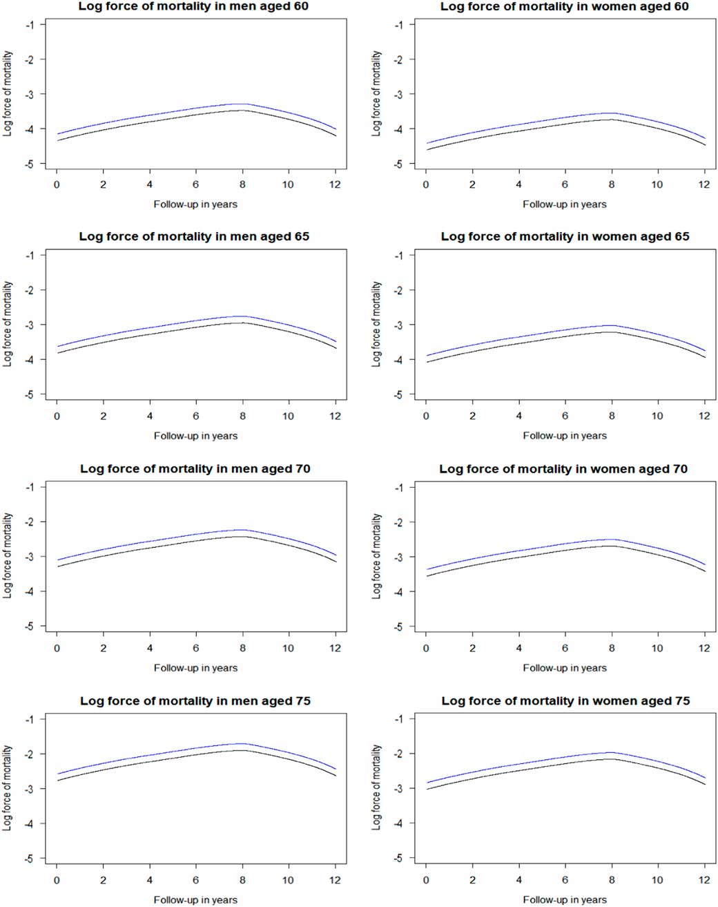
Figure 5 Log force of mortality in hypertensive patients on standard treatment (black) and on intensive treatment (blue) by sex and age. Log force of mortality adjusted for deprivation (reference of 3rd Index of Multiple Deprivation quintile), lifestyle factors (reference of healthy), and medical history (reference of healthy). Standard treatment has a systolic blood pressure target of ≤140 mmHg, whereas intensive treatment has a target of ≤120 mmHg.
The overall period life expectancy of hypertensive people can be calculated using the prevalence of hypertension, the requisite hazard ratios, and the overall period life expectancy in the general population. In the next step, the period life expectancies of hypertensive people on standard blood pressure treatment and those on intensive blood pressure treatment can be calculated using the prevalence of intensive blood pressure treatment in hypertensive people (Table 4), the requisite hazard ratios and the overall period life expectancy of hypertensive people (obtained from the previous step). Table 5 presents these calculated period life expectancies at chronological ages 60, 65, 70 and 75 by sex.
Table 4 Prevalence of the Intensive Treatment of Blood Pressure in the Study Sample
Author’s computations.
Table 5 Period Life Expectancy for People With High Blood Pressure at 2010 Prevalence of Intensive Blood Pressure Treatment and Period Life Expectancies for People with High Blood Pressure on Intensive or Standard Treatment
The period life expectancies (95% confidence intervals (CI)) are based on the UK life table centred 2009–2011 (Office for National Statistics, 2017).
* Period life expectancy for people with high blood pressure at 2010 prevalence of intensive blood pressure treatment. This period life expectancy is the weighted average of the next two period life expectancies:
† Period life expectancy for people with high blood pressure on intensive treatment.
‡ Period life expectancy for people with high blood pressure on standard treatment.
Hypothetical changes in the population life expectancy of people with hypertension can be derived from changes in the prevalence of intensive blood pressure treatment. For example, if all men with hypertension at age 60 would be on the intensive blood pressure treatment, then their population life expectancy would decrease from 20.0 to 18.6 years, while if all would be on the standard blood pressure treatment, their population life expectancy would increase to 20.7 years. Similarly, for women with hypertension at age 60, if all would be on the intensive blood pressure treatment, their population life expectancy would decrease from 23.0 to 21.5 years, while if all would be on the standard blood pressure treatment, their population life expectancy would increase to 23.8 years.
7. Comment About Using Estimated Hazards from Medical Studies
One should be cautious in taking estimated hazards of mortality in medical studies at face value and translating them directly to life expectancies at the individual and population levels. As was shown in the last example, the SPRINT clinical trial estimated a decrease in effective age of 3.4–3.6 years in hypertensive patients due to the intensive blood pressure treatment compared to the standard blood pressure treatment. Given the public health impact of the recent AHA guidelines, this would predict a considerable boost to the life expectancy in the United States. In contrast, our observational cohort study estimated an increase in effective age of 1.7–1.8 years in hypertensive patients due to the intensive blood pressure treatment. This well may be due to the high heterogeneity of the general population. Medical studies should be evaluated on the reliability and generalisability of the results to the general population before translating the estimated hazards of mortality to changes in life expectancy. Examples that could affect the reliability and generalisability of the results are the selection criteria of the sample, the sample size, the length of follow-up, the measurement of risk factors, the presence of confounding risk factors, and the appropriateness of statistical methods.
8. Conclusion
This paper demonstrated how hazards of mortality can be translated to life expectancies at the individual and population levels. The information needed to calculate these life expectancies is the hazard of mortality associated with the risk factor of interest, the prevalence of the risk factor of interest, and a life table of the underlying population.
In both examples, hypothetical changes in the subpopulation life expectancy were derived from changes in the prevalence of the health conditions and/or interventions of interest. So the assumptions need to be made only about possible trends in prevalence, as the magnitude of an effect of a disease or a treatment on life expectancy would be already established from the described analysis.
In this vein, in the beta blockers example, hypothetical changes in the overall life expectancy of heart attack survivors were derived from changes in the prevalence of prescription of beta blockers in this group. For example, if all men surviving a heart attack by age 60 were to be prescribed beta blockers, then their population life expectancy would increase from 17.4 to 18.8 years, while if none were prescribed the drugs, their population life expectancy would decrease to 16.4 years. But if the prescription rate is assumed to increase, say, to 80% (a more realistic assumption), then their population life expectancy would increase from 17.4 to 18.3 years. Similarly, for women surviving a heart attack by age 60, if all were prescribed beta blockers, their population life expectancy would increase from 20.3 to 21.8 years, while none were prescribed the drugs, their population life expectancy would decrease to 19.3 years. At 80% prescription, their population life expectancy would increase to 21.1 years.
In this Research Programme, funded by the Actuarial Research Centre, we have already investigated changes in life expectancy to do with statins (Gitsels et al., Reference Gitsels, Kulinskaya and Steel2016), various heart attack treatments (Gitsels et al., Reference Gitsels, Kulinskaya and Steel2017) and alternative blood pressure targets (Gitsels et al., 2018). We have also started work on (1) diabetes, one of the main killers of the 21st century, (2) stroke, which can have great implications for life, health and long-term care insurance, and (3) hormone replacement therapy, an intervention which greatly affects lifestyle, morbidity and possibly longevity of the female population.
Changes in the prevalence of the risk factor of interest are reflected in the life expectancy at the population level. From this, it can be calculated how much the risk factor of interest has already contributed in changes in past longevity improvements and how continuing trends of the prevalence of the risk factor of interest can affect future life expectancy. These calculations can be informative for mortality projections of populations of insureds and pension schemes.
Allowing for changes in prevalence in known treatments (e.g. anti-hypertensive prescriptions) and differences in other factors (e.g. socioeconomic status) will never provide a complete answer, however, especially when projecting future mortality improvements. It is a useful tool, though, that can also help with questions like: “What would be the impact of another medical advance the size of statins?”
Acknowledgements
The authors acknowledge funding from the Actuarial Research Centre of the Institute and Facility of Actuaries through the “Use of Big Health and Actuarial Data for understanding Longevity and Morbidity Risks” research programme. The work by L.A.G. was supported by the Economic and Social Research Council [grant number ES/L011859/1]. The authors also thank Prof Andrew Cairns for his useful suggestions for improving the presentation of the material of this article.


 Open access