


1. Introduction
Liquid jets with non-straight trajectories appear in many industrial applications, including fibre spinning (Mellado et al. Reference Mellado, McIlwee, Badrossamay, Goss, Mahadevan and Kit Parker2011), centrifugal hydrogel synthesis (Eral et al. Reference Eral, Safai, Keshavarz, Kim, Lee and Doyle2016) and homogenization (Singh et al. Reference Singh, Gupta, Buchner, Ibis, Pronk, Tam and Eral2019), spinning disc atomization (Li, Sisoev & Shikhmurzaev Reference Li, Sisoev and Shikhmurzaev2018; Keshavarz et al. Reference Keshavarz, Houze, Moore, Koerner and McKinley2020) and prilling (Decent, King & Wallwork Reference Decent, King and Wallwork2002; Saleh et al. Reference Saleh, Ahmed, Al-mosuli and Barghi2015). In spinning disc atomization and prilling, the product yields are the droplets/prills formed under inertio-capillary breakup of a spiralling jet, mainly due to a Rayleigh–Plateau instability. To better control the breakup and drop formation process of a spiralling jet, one needs a thorough understanding of the jet flow along a helical trajectory, i.e. how an instability evolves downstream and leads to breakup, as well as experimental validation of the proposed theories and results. The rotating nature of the spiralling jet makes it rather challanging to design set-ups where the experimental conditions are precisely controlled. Wong et al. (Reference Wong, Simmons, Decent, Părău and King2004) studied spiralling jets experimentally, where the jet was issued from an orifice on a rotating bucket that is drained by hydrostatic pressure due to gravity and rotation. They discuss the combined effect of gravity and rotation on the exit velocity and provided observations on the breakup modes corresponding to different non-dimensional numbers. In a follow-up study, Partridge et al. (Reference Partridge, Wong, Simmons, Părău and Decent2005) studied spiralling jets on a bigger set-up and highlighted that, for a larger set-up, it is harder to predict the breakup characteristics as mechanical vibrations and air resistance plays a much bigger role. In addition to experimental approaches, analytical models were also developed. Wallwork et al. (Reference Wallwork, Decent, King and Schulkes2002) studied spiralling jets extensively in the inviscid limit, providing temporal and spatial linear stability analyses along with it. This was later extended to include viscous effects (Părău et al. Reference Părău, Decent, Simmons, Wong and King2007; Decent et al. Reference Decent, King, Simmons, Părău, Wallwork, Gurney and Uddin2009; Marheineke & Wegener Reference Marheineke and Wegener2009), non-Newtonian fluid behaviour (Uddin, Decent & Simmons Reference Uddin, Decent and Simmons2006; Alsharif, Uddin & Afzaal Reference Alsharif, Uddin and Afzaal2015) and Marangoni effects from surfactants (Alsharif & Uddin Reference Alsharif and Uddin2015). In an extensive mathematical study, Shikhmurzaev & Sisoev (Reference Shikhmurzaev and Sisoev2017) pointed out how a priori assumptions in the definition of the jet specific coordinate frame lead to an erroneous derivation of the base jet trajectory equations and they laid out a curvilinear local coordinate framework without any assumptions. This approach was later applied by Li, Sisoev & Shikhmurzaev (Reference Li, Sisoev and Shikhmurzaev2019) and Noroozi et al. (Reference Noroozi, Arne, Larson and Taghavi2020) to study the trajectory and the base flow of a spiralling jet.
Comparison of the predictions from linear stability analyses with experiments revealed their lack of ability to predict the jet behaviour at later stages of instability and the subsequent drop formation, stressing the necessity of a nonlinear modelling approach. However, full three-dimensional (3-D) simulations of the breakup of a spiralling jet would be computationally very expensive and is not feasible yet. Li et al. (Reference Li, Sisoev and Shikhmurzaev2019) have used an arbitrary Lagrangian–Eulerian based ‘end code’ where the prescribed base flow trajectory (and, thus, the locally varying body forces in a curvilinear system describing the jet) are used to simulate the nonlinear stages of the growth of perturbations. By exploiting the typically slender nature of the spiralling jets, the nonlinear growth can be accurately simulated with a one-dimensional (1-D) slender-jet model (Eggers & Dupont Reference Eggers and Dupont1994) in which the spiralling jet is basically treated as a quasi-straight jet with locally varying body forces. The strength of the slender-jet approach has been showcased in several studies on nozzle driven jets; Driessen et al. (Reference Driessen, Sleutel, Dijksman, Jeurissen and Lohse2014) showed droplet regime control using multimode perturbations and McIlroy & Harlen (Reference McIlroy and Harlen2019) studied the effects of finite perturbation amplitude on breakup characteristics. The method proved useful also in non-isothermal cases with the additional presence of thermo-capillary (Marangoni) effects (Pillai et al. Reference Pillai, Narayanan, Pushpavanam, Sundararajan, Jasmin Sudha and Chellapandi2012; Kamis, Eral & Breugem Reference Kamis, Eral and Breugem2021).
The case of a spiralling jet bears many analogies to straight jets under a non-negligible gravity force, since the fictitious forces that dictate the trajectory of the jet have finite longitudinal projections that stretch the jet along the flow direction. It is well known that the Rayleigh–Plateau instability is significantly altered by the presence of stretching (Tomotika Reference Tomotika1936). In the context of gravity-driven jets, the regimes are studied in both the viscous (Sauter & Buggisch Reference Sauter and Buggisch2005; Javadi et al. Reference Javadi, Eggers, Bonn, Habibi and Ribe2013) and the inviscid limit (Le Dizès & Villermaux Reference Le Dizès and Villermaux2017). On the one hand, stretching tends to damp the perturbations when the time scale related to stretching is much faster than that of the inertio-capillary growth (Eggers & Villermaux Reference Eggers and Villermaux2008). On the other hand, stretching tends also to enhance perturbations through thinning of the jet and the associated reduction of the inertio-capillary time scale along the jet.
Previous studies on the effect of stretching in gravity-driven and spiralling jets have mainly been on the linear stability analyses under infinitesimally small perturbations. A full overview on the process from initial perturbation till jet breakup and beyond, including further breakup or coalescence of detached drops, is missing. Here we present results from a comprehensive study on the breakup of spiralling jets based on experiments, nonlinear slender-jet simulations and linear stability analysis. Our prime interest is in accurate estimation of the breakup of a spiralling jet and resultant drop size distribution and to provide physical insights for practical applications of this complex problem.
In § 2 we provide details on the experimental set-up used. In § 3 we present the nonlinear slender-jet model, including details of the underlying mathematical framework and a derivation of the base flow equations. Results for the jet breakup from the experiments and the slender-jet model are discussed in § 4. In the next section we demonstrate the analogy between a spiralling jet in the presence of fictitious forces and a straight jet subject to gravity. This is used then in a linear stability analysis with an integrated gain approach (Javadi et al. Reference Javadi, Eggers, Bonn, Habibi and Ribe2013; Le Dizès & Villermaux Reference Le Dizès and Villermaux2017). Furthermore, in analogy with a gravity-driven straight jet, we show the existence of similarity solutions. Finally, in § 6 we draw the main conclusions.
2. Experimental set-up
The computer-aided design (CAD) model and the schematic of the experimental set-up are shown in figure 1. A fluid reservoir with a nearly constant pressure head delivers the fluid to the rotating nozzle via an intermediate chamber. A rotary swivel joint is used to connect the stationary fluid chamber to the rotating nozzle. The swivel joint is spun with a stepper motor through a timing belt at the desired speed. A circular plate connected to the piezo actuator is embedded in the fluid chamber for a well-controlled periodic perturbation of the nozzle exit velocity at a desired frequency. The jet is visualised with the help of a high-speed camera that is fixed in the lab frame of reference. The camera records at a frequency of 2500 frames per second to capture consecutive breakup events. The pixel size of the sensor is  $11 \times 11 \,\mathrm {\mu }{\rm m}^2$ and the scale factor was found to be of $53\,\mathrm {\mu } {\rm m}\,{\rm px}^{-1}$, which corresponds to a magnification of 0.207. The exposure time of the camera is set to $75\,\mathrm {\mu }{\rm s}$, which limits the blurring of the jet to around 1.6 px. Since the Rossby number is close to unity, the blurring due to streamwise motion and the rotation of the jet is similar. Completely eliminating blurring was not possible so a compromise was made between blurring and good contrast. The jet is illuminated from the back by a LED panel. The velocity of the jet is determined at an estimated accuracy of $2\,\%$ from the drop in liquid level of the fluid reservoir. Properties of the working fluid are given in table 1.

Figure 1. Experimental set-up. (a) Schematic of the set-up. (b) A CAD drawing of the piezo actuator and plate, fluid discharge tank and the rotary elbow. (c) Photo of the parts given in (b).
Table 1. Experimental parameters and corresponding non-dimensional numbers used in the simulations.

3. Computational model
We performed a numerical study of the same flow geometry as considered in the experiments. The flow within the jet is decomposed into two components, namely, a stationary base state and perturbation. The perturbations are imposed at the nozzle and they evolve downstream along the jet. The jet trajectory and base flow are coupled with each other and, hence, must be solved simultaneously. Using the knowledge of the trajectory and how the jet velocity evolves downstream, we can then consider the perturbations on the jet. In what follows, we first present the mathematical framework in which we derive the governing equations in a moving frame of reference using curvilinear coordinates. Assuming a slender jet, we then derive the equations for the base flow and compute from this the fictitious forces acting on the flow along the jet trajectory. Finally, we derive the slender-jet model for the flow perturbations.
3.1. Mathematical framework
In a frame of reference co-rotating with the nozzle at an angular velocity  $\boldsymbol {\varOmega } = (0,0,-\varOmega )$, the non-dimensional Navier–Stokes equations for the Newtonian liquid flow in the jet read
 $$\begin{gather} \boldsymbol{\nabla}\boldsymbol{\cdot}\boldsymbol{u} = 0, \end{gather}$$
 $$\begin{gather}\frac{{\rm D}\boldsymbol{u}}{{\rm D}t} ={-}\boldsymbol{\nabla} p + \frac{1}{Re}\boldsymbol{\nabla}\boldsymbol{\cdot}\left(2\boldsymbol{\mathsf{D}}\right) - \frac{1}{{\textit{Rb}}^2}\boldsymbol{\varOmega}\times\left(\boldsymbol{\varOmega}\times\boldsymbol{d}\right) - \frac{2}{{\textit{Rb}}} \boldsymbol{\varOmega}\times\boldsymbol{u} + \frac{1}{{\textit{Fr}}^2} \boldsymbol{g}, \end{gather}$$
where  $\boldsymbol {g} = (0,0,-g)$ and $\boldsymbol{\mathsf{D}}=(\boldsymbol {\nabla }\boldsymbol {u}+\boldsymbol {\nabla }\boldsymbol {u}^{\rm T})/2$ is the rate-of-strain tensor and $\boldsymbol {d}$ is the distance vector with respect to the rotating axis. The definitions and values of the non-dimensional numbers are provided in table 1. The mathematical framework we use is very similar to what is described in detail in Shikhmurzaev & Sisoev (Reference Shikhmurzaev and Sisoev2017) and Noroozi et al. (Reference Noroozi, Arne, Larson and Taghavi2020), but briefly revisited here for completeness. Figure 2 shows a schematic of a curved jet. We start by describing a baseline (Shikhmurzaev & Sisoev Reference Shikhmurzaev and Sisoev2017), which is a spline that goes along the jet and remains inside it, using Cartesian basis vectors on a frame rotating with $\varOmega$ (see figure 2a),
 \begin{equation} \boldsymbol{D}(s) = X(s) \boldsymbol{\hat{x}} + Y(s) \boldsymbol{\hat{y}} + Z(s) \boldsymbol{\hat{z}}, \end{equation}
where  $s$ is the arclength. From (3.2) the Frenet basis can be defined, i.e. a local orthogonal basis defined at every point on the baseline,
 $$\begin{gather} \boldsymbol{T}(s) = \frac{{\rm d}\boldsymbol{D}}{{\rm d}s} = X'(s)\boldsymbol{\hat{x}}+Y'(s)\boldsymbol{\hat{y}}+Z'(s)\boldsymbol{\hat{z}} \quad \left(X'^2 +Y'^2 + Z'^2 = 1\right), \end{gather}$$
 $$\begin{gather}\boldsymbol{N}(s) = \frac{{\rm d}\boldsymbol{T}}{{\rm d}s}\left\lvert\frac{{\rm d}\boldsymbol{T}}{{\rm d}s}\right\rvert^{{-}1}=\frac{X''\boldsymbol{\hat{x}}+Y''\boldsymbol{\hat{y}}+Z''\boldsymbol{\hat{z}}}{\sqrt{X''^2+Y''^2+Z''^2}}, \end{gather}$$
 $$\begin{gather}\boldsymbol{B}(s) = \boldsymbol{T}\times\boldsymbol{N}, \end{gather}$$
where a prime denotes derivative with respect to  $s$. The derivatives of the Frenet base vectors are related to each other by the Frenet formulas
 \begin{equation} \frac{{\rm d}}{{\rm d}s}\left[{\begin{array}{@{}c@{}} \boldsymbol{T} \\ \boldsymbol{N} \\ \boldsymbol{B} \end{array}}\right] = \left[{\begin{array}{@{}ccc@{}} 0 & \kappa & 0 \\ -\kappa & 0 & \tau \\ 0 & -\tau & 0 \end{array}}\right] \left[{\begin{array}{@{}c@{}} \boldsymbol{T} \\ \boldsymbol{N} \\ \boldsymbol{B} \end{array}}\right]. \end{equation}
Here  $\kappa (s)$ and $\tau (s)$ are, respectively, the local curvature and the local torsion of the baseline, given by
 $$\begin{gather} \kappa(s) = \sqrt{X''^2+Y''^2+Z''^2}, \end{gather}$$
 $$\begin{gather}\tau(s) = \frac{X'(Y''Z'''-Z''Y''')+Y'(Z''X'''-X''Z''')+Z'(X''Y'''-Y''X''')}{(Y'Z''-Z'Y'')^2+(Z'X''-X'Z'')^2+(X'Y''-Y'X'')^2}. \end{gather}$$
Let us now define the curvilinear coordinate variables,  $(s,r,\phi )$, where $s$ is again the arc length variable, and $(r,\phi )$ are the polar radius and angle, respectively, on the plane that is normal to the baseline at $\boldsymbol {D}(s)$. Note from the definition of the Frenet basis (3.3) that this is also the plane where $\boldsymbol {N}(s)$ and $\boldsymbol {B}(s)$ lie. So we can define an arbitrary point in the jet with a position vector measured from the origin in the Cartesian and curvilinear coordinates as follows:
 $$\begin{gather} \boldsymbol{d}(x,y,z) = x\boldsymbol{\hat{x}} + y\boldsymbol{\hat{y}} +z\boldsymbol{\hat{z}}, \end{gather}$$
 $$\begin{gather}\boldsymbol{d}(s,r,\phi) = \boldsymbol{D}(s) + r\cos{\phi}\boldsymbol{N}(s) +r\sin{\phi}\boldsymbol{B}(s). \end{gather}$$
Figure 2. (a) Schematic of the top view of the set-up. (b) Close-up view of a section in the jet showing the different coordinate frames.
The free surface can be parametrically described as  $r = R(s,\phi )$, with which the position vector to the free surface takes the form
 \begin{equation} \boldsymbol{d}(s,R(s,\phi),\phi) = \boldsymbol{D}(s) + R(s,\phi)\cos{\phi}\boldsymbol{N}(s) +R(s,\phi)\sin{\phi}\boldsymbol{B}(s). \end{equation}
On the free surface one has the balance of stresses in the normal and tangential directions,
 $$\begin{gather} \boldsymbol{n}\boldsymbol{\cdot}\left({-}p+\frac{1}{Re}2\boldsymbol{\mathsf{D}}\right)\boldsymbol{\cdot} \boldsymbol{n} ={-}\frac{1}{{\textit{We}}}\kappa_{\textit{fs}}, \end{gather}$$
 $$\begin{gather}\boldsymbol{t_i}\boldsymbol{\cdot}\left({-}p+\frac{1}{Re}2\boldsymbol{\mathsf{D}}\right)\boldsymbol{\cdot}\boldsymbol{n} = 0, \quad i = s,\phi, \end{gather}$$
where  $\kappa _{\textit {fs}}$ is the curvature of the free surface. Here, the ambient phase is assumed to be dynamically inert and the effect of air drag is neglected.
We will use the notation  $(s^1, s^2, s^3) = (s,r,\phi )$ to define the base vectors of the curvilinear coordinate frame as
 \begin{equation} \boldsymbol{e}_i = \frac{\partial \boldsymbol{d}}{\partial s^i} \quad (i=1,2,3). \end{equation}
Using (3.9), we can now express curvilinear base vectors in terms of the Frenet frame as follows:
 \begin{equation} \left[{\begin{array}{@{}c@{}} \boldsymbol{e}_1 \\ \boldsymbol{e}_2 \\ \boldsymbol{e}_3 \end{array}}\right] = \left[{\begin{array}{@{}ccc@{}} 1-r\kappa\cos{\phi} & -r\tau\sin{\phi} & r\tau\cos{\phi} \\ 0 & \cos{\phi} & \sin{\phi} \\ 0 & -r\sin{\phi} & r\cos{\phi} \end{array}}\right] \left[{\begin{array}{@{}c@{}} \boldsymbol{T} \\ \boldsymbol{N} \\ \boldsymbol{B} \end{array}}\right]. \end{equation}
 The metric of this basis,  $\boldsymbol{\mathsf{g}}$, defined as $g_{ij} = \boldsymbol {e_i \boldsymbol {\cdot} e_j}$, is given by
 \begin{equation} \boldsymbol{\mathsf{g}} = \left[{\begin{array}{@{}ccc@{}} (1-r\kappa\cos{\phi})^2 + (r\tau)^2 & 0 & r^2\tau \\ 0 & 1 & 0 \\ r^2\tau & 0 & r^2 \end{array}}\right]. \end{equation}
 Note that the coordinate frame defined by (3.9) is not orthogonal as  $g_{13}$ and $g_{31}$ are not zero in the presence of torsion or outside the baseline ( $r\neq 0$). Another aspect of the curvilinear base is that two base vectors, namely $\boldsymbol {e}_1$ and $\boldsymbol {e}_3$, are not unit vectors since $g_{11}\neq 1$ and $g_{33}\neq 1$. As a consequence, there is a change in magnitude when a vector $\boldsymbol {v}=(v^1,v^2,v^3)$ is projected onto the curvilinear base. For instance, the projection of the velocity vector $\boldsymbol {u}$ on the curvilinear base is represented by $v^1\boldsymbol {e}_1+v^2\boldsymbol {e}_2+v^3\boldsymbol {e}_3 = u_s\boldsymbol {e}_1/|\boldsymbol {e}_1|+u_r\boldsymbol {e}_2/|\boldsymbol {e}_2|+u_{\phi }\boldsymbol {e}_3/|\boldsymbol {e}_3|$, where $u_s$, $u_r$ and $u_{\phi }$ are the physical components of the velocity using the normalized base vectors.
The inverse metric tensor ( $g^{ij}$) is defined by $g^{ik}g_{kj}=\delta _j^i$, where $\delta _j^i$ is Kronecker delta, and is given by
 \begin{equation} \boldsymbol{\mathsf{g}}^{{-}1} = \frac{1}{\varDelta}\left[{\begin{array}{@{}ccc@{}} r^2 & 0 & -r^2\tau \\ 0 & \varDelta & 0 \\ -r^2\tau & 0 & (1-r\kappa\cos{\phi})^2 + (r\tau)^2 \end{array}}\right], \end{equation}
with  $\varDelta = \det (g_{ij}) = r^{2} (r \kappa {(s )} \cos {(\phi )} - 1)^{2}$ the determinant of the metric tensor.
Using the metric and its inverse, we can express the gradient operator as (Wesseling Reference Wesseling2009)
 \begin{equation} \boldsymbol{\nabla} = g^{ij}\boldsymbol{e}_j\frac{\partial}{\partial s^i} = \left(\frac{1}{e_{1T}^2}\frac{\partial}{\partial s}-\frac{\tau}{e_{1T}^2}\frac{\partial}{\partial \phi}\right)\boldsymbol{e}_1 + \frac{\partial}{\partial r}\boldsymbol{e}_2 + \left(\frac{g_{11}}{r^2 e_{1T}^2}-\frac{\tau}{e_{1T}^2}\right)\boldsymbol{e}_3, \end{equation}
with  $g_{11}=(1-r\kappa \cos {\phi })^2 + (r\tau )^2$ being the first element of the metric tensor given in (3.11) and $e_{1T}=1-r\kappa \cos {\phi }$ is the tangential component of the local base vector in the $s$ direction, namely the first element of the transformation matrix given in (3.10).
Finally, the coefficients to connect the variations of the base state vectors (also known as the Christoffel symbols of the second kind  $\varGamma ^k_{ij}$, such that ${\partial \boldsymbol {e}_i}/{\partial s^j} = \varGamma ^k_{ij}\boldsymbol {e}_k$) can be written as
 \begin{equation} \varGamma^k_{ij} = \frac{g^{kl}}{2}\left(\frac{\partial g_{lj}}{\partial s^i}+\frac{\partial g_{li}}{\partial s^j}-\frac{\partial g_{ij}}{\partial s^l}\right). \end{equation}
The full expressions of each Christoffel symbol are provided in Appendix C. From here onwards, it is tedious book keeping to determine the terms in (3.1a) and (3.1b) in curvilinear coordinates. This was achieved by the help of the symbolic mathematics module SymPy (Meurer et al. Reference Meurer2017). Some of the terms in the conservation equations in general curvilinear coordinates are provided in Appendix C.
To pave the way for the slender-jet approximation, one needs to acknowledge the existence of two disparate length scales existing in the problem. These are namely the rotating arm,  $L$, and the orifice radius, $R_0$. We scale $s$ with $L$ and $r$ with $R_0$. The velocity at the orifice, $U_0$, is used for scaling the velocity in the $s$ direction, so the advective time scale becomes $t_{\textit {adv}} = L/U_0$. Finally, the pressure is scaled with $\rho U_0^2$.
3.2. Jet trajectory and base flow
To obtain the leading order steady state equations for the spiralling jet trajectory, one needs to consider the limit where the jet slenderness  $\epsilon$ tends to zero, i.e. $R_0/L\rightarrow 0$. The steady state jet base flow equations, namely, the mass conservation, the projections of the momentum conservation in tangential, normal and binormal directions and the arc length condition have the following form:
 \begin{gather} \frac{{\rm d}}{{\rm d}s}\left(UR^2\right) = 0, \end{gather}
 \begin{gather} U\frac{{\rm d}U}{{\rm d}s} ={-}\frac{1}{{\textit{We}}}\frac{{\rm d}}{{\rm d}s}\left(\frac{1}{R}\right) + \frac{3}{R^2Re}\frac{{\rm d}}{{\rm d}s}\left(R^2 \frac{{\rm d}U}{{\rm d}s}\right) \underbrace{-\frac{Z'}{{\textit{Fr}}^2}}_{f_{\textit{gravity}}} + \underbrace{\frac{XX'+YY'}{{\textit{Rb}}^2}}_{f_{\textit{centrifugal}}}, \end{gather}
 $$\begin{gather} \left(U^2-\frac{1}{RWe}-\frac{3}{Re}\frac{{\rm d}U}{{\rm d}s}\right)\left(X''^2+Y''^2+Z''^2\right) = \frac{XX''+YY''}{{\textit{Rb}}^2}\nonumber\\ - \frac{2U\left(X'Y''-Y'X''\right)}{{\textit{Rb}}} - \frac{Z''}{{\textit{Fr}}^2}, \end{gather}$$
 \begin{gather} 0 = \frac{X\left(Y'Z''-Z'Y''\right)+Y\left(Z'X''-X'Z''\right)}{{\textit{Rb}}^2} - \frac{X'Y''-Y'X''}{{\textit{Fr}}^2} + \frac{2UZ''}{{\textit{Rb}}}, \end{gather}
 \begin{gather} X'^2+Y'^2+Z'^2 = 1. \end{gather}
These equations form a closed system for  $X(s)$, $Y(s)$, $Z(s)$, the Cartesian coordinates of the baseline of the jet, and $R(s)$, $U(s)$, which express the local velocity and jet thickness. The factor 3 in front of the second term on the right-hand side of (3.16) is the Trouton number that represents the ratio of extensional to shear viscosity. It appears naturally in the asympotic expansion of the governing equations. In the inviscid limit ( ${\textit {Re}} \gg 1$), which approximately hold for our experiments, (3.16) can be combined in a single integrand and readily integrated as
 \begin{equation} U^2+\frac{2U^{1/2}}{{\textit{We}}\sqrt{C_1}}+\frac{2}{{\textit{Fr}}^2}Z-\frac{1}{{\textit{Rb}}^2}\left(X^2+Y^2\right) + C_2 = 0, \end{equation}
where we used  $UR^2=C_1$ from (3.15), and $C_1$ and $C_2$ are integration constants. Note that viscous resistances to bending and twisting are also neglected in this case.
The rotation path of the orifice lies on the  $XY$ plane, as shown in figure 2(a). We define $X(0)=1$, $Y(0)=0$, $Z(0)=0$, $X'(0)=1$, $Y'(0)=0$ and finally $Z'(0)$ from (3.19), i.e. the jet is issued in the $X$ direction. The nozzle velocity $U_0$ and the radius $R_0$, which have been used for non-dimensionalization, set the base flow boundary conditions as $U(0)=R(0)=1$ and, hence, $C_1=1$. Combining all the prescribed boundary conditions in (3.20) yields $C_2 = 1/{\textit {Rb}}^2 - 2/{\textit {We}} - 1$.
We solve the system (3.15), (3.17)–(3.20), also known as the ‘string’ equations, with the prescribed boundary conditions and the non-dimensional numbers given in table 1 using a fourth-order Runge–Kutta method. The results are summarized in figure 3. The base jet trajectory is in great agreement with the experiments, so it enables the quantification of the projections of the body forces along the trajectory, namely, the centrifugal force,  $\,f_{\textit {centrifugal}}(s)$, and gravity force, $\,f_{\textit {gravity}}(s)$, whose expressions are given on the right-hand side of (3.16). Figure 3 depicts the results from the base flow calculations. It is apparent that with the parameters in our experiment, the gravity force is about an order of magnitude smaller than the centrifugal force, which suggests that the torsion along the arc length and distance travelled by the jet in the $Z$ direction are negligibly small, allowing us to study the dynamics from two-dimensional projections onto the $XY$ plane.

Figure 3. Results from the base flow computation. (a) Comparison of calculated jet trajectory (red line) with a snapshot from an unperturbed jet experiment. (b) The variation of the base state velocity,  $U(s)$, and jet radius, $R(s)$, along the jet. (c) The variation of the body forces acting along the jet due to rotation $\,f_{\textit {centrifugal}}=(XX'+YY')/{\textit {Rb}}^2$ and gravity $\,f_{\textit {gravity}}=-Z'/{\textit {Fr}}^2$.
3.3. Nonlinear slender-jet model
To be able to capture the dynamics close to breakup, e.g. the formation of main and satellite droplets, nonlinear simulations are necessary. Once the longitudinal projections of the centrifugal and the gravity forces are accounted for, one can approximate the nonlinear dynamics of the jet along the flow direction with an error of  ${O}(\epsilon )$, provided that the full free surface curvature is accounted for (Li et al. Reference Li, Sisoev and Shikhmurzaev2019). In other words, the 3-D spiralling trajectory of the jet can be represented as a quasi-straight jet with locally varying body forces. This also amounts to the implicit assumption that the wavenumber of the perturbations $k$ (scales with $R_0^{-1}$) is much larger than the curvature $\kappa$ and the torsion $\tau$ of the base jet trajectory (both scale with $L^{-1}$) that is valid in the limit $\epsilon \rightarrow 0$. To this end, we implemented a slender-jet approximation, detailed in Eggers & Dupont (Reference Eggers and Dupont1994) and Kamis et al. (Reference Kamis, Eral and Breugem2021), which yields the following unsteady 1-D equations for the jet flow:
 $$\begin{gather} \frac{\partial A}{\partial t}+\frac{\partial}{\partial s}\left(u A\right) = 0, \end{gather}$$
 $$\begin{gather}\frac{\partial \left(uA\right)}{\partial t} + \frac{\partial}{\partial s}\left(u^2 A\right) = \frac{\partial}{\partial s}\left[A\left(\frac{K}{{\textit{We}}}+\frac{3\epsilon}{{\textit{Re}}}\frac{\partial u}{\partial s}\right)\right] + A\left[\epsilon\left(\,f_{\textit{centrifugal}}+\,f_{\textit{gravity}}\right)\right], \end{gather}$$
 $$\begin{gather}K = \frac{2}{\sqrt{4A+A_{\textit{s}}^2}}+\frac{4AA_{\textit{ss}}-2A_s^2} {\left(4A+A_{\textit{s}}^2\right)^{3/2}}. \end{gather}$$
Here  $A=R^2$ is the normalized local jet cross-sectional area. Note that the full expression for the curvature is used (i.e. both radii of curvature instead of only the leading order one in the expansion). This is key to the success of the slender-jet framework (Entov & Yarin Reference Entov and Yarin1984; Ambravaneswaran, Wilkes & Basaran Reference Ambravaneswaran, Wilkes and Basaran2002).
Note the inclusion of the  $\epsilon$ parameter in front of the centrifugal and gravity force in (3.21b) as they have been taken from (3.16) and are hence normalised with $L$ instead of $R_0$. Equations (3.21) form a closed system for the jet cross-sectional area $A(s,t)$ and jet velocity $u(s,t)$. The initial conditions are implemented as $A(s,0) = R(s)^2$ and $u(s,0) = U(s)$ from the base flow computations detailed in § 3.2. At the nozzle, we input the velocity fluctuations as $u(0,t) = 1+\varepsilon _v \cos {(\omega t)}$ on top of the Gaussian white noise that is mentioned in § 4. A regularized capillary pressure is implemented to carry the simulations beyond the pinch-off point (Driessen & Jeurissen Reference Driessen and Jeurissen2011). A finite difference scheme on a staggered grid is used for solving the system given in (3.21). The time integration is done explicitly by using a three-step Runge–Kutta scheme with an adaptive time stepping. Except for velocities, a central differencing scheme is used for evaluating the variables at their half-step neighbours. For velocities, a higher-order total variation diminishing van Leer scheme is used. More details of the numerical method and validation can be found in Kamis et al. (Reference Kamis, Eral and Breugem2021).
Mechanical vibrations are naturally present in industrial applications of spiralling jets such as in prilling, where the typical size of the rotating perforated bucket is of the order of 50 cm. Even in small-scale laboratory experiments, one can never get fully rid of such vibrations, and they might have a significant effect on the jet breakup. The time series of such noisy perturbations are rather difficult to quantify, however, a good proxy is to represent the vibrations by white noise and to characterize the noise strength in terms of the natural (actuation-free) jet breakup length or breakup time (Pimbley & Lee Reference Pimbley and Lee1977).
To simulate the natural breakup in the slender-jet framework, we add Gaussian white noise to the nozzle velocity as follows:
 \begin{equation} u(0,t) = 1 + \underbrace{\varepsilon_v \cos{(\omega t)}}_{\text{perturbation}} + \underbrace{W(\Delta t)}_{\text{white noise}}. \end{equation}
The white noise is generated using standard random number generators in Matlab and its standard deviation scales as  $S\Delta t$, where $S$ is a strength parameter and $\Delta t$ is the computational time step. This ensures that the forcing due to the white noise is uncorrelated with the time step (Kamis et al. Reference Kamis, Eral and Breugem2021). The strength parameter $S$ is then calibrated using the observed experimental natural (i.e. $\varepsilon _v=0$) breakup length. In the present study we subsequently used $S=300$ in all simulations and the non-dimensional time step $\Delta t$ is adjusted dynamically considering the stability restrictions based on the effects of advection, diffusion and surface tension (Brackbill, Kothe & Zemach Reference Brackbill, Kothe and Zemach1992; Wesseling Reference Wesseling2009).
The comparison of the simulation and experiments for the parameters listed in table 1 and in the presence of only background noise, is summarized in table 2.
Table 2. Mean and standard deviation of the breakup properties of natural (actuation-free) breakup cases. The breakup length is expressed in terms of the nozzle radius  $R_0$ and the drop projected area is represented in terms of $R_0^2$.

4. Comparison of simulations with experiments for jet breakup
Simulations and experiments have been conducted for the parameter settings listed in table 1 and for three different actuation frequencies ( $\omega$). The strength of perturbations was varied by varying the velocity perturbation amplitude ( $\varepsilon _v$) in the simulations and the oscillation amplitude of the piezo actuator ( $\Delta h_{\textit {piezo}}$) in the experiments. The simulation results from the slender-jet model for the jet interface have been projected from the curvilinear to the Cartesian frame using 3.7. Figure 4(a) shows the comparison of a slender-jet simulation and an experiment at $\omega =0.7$ and in figure 4(b) we show the change in the mean intact length with respect to the perturbation amplitude at different frequencies. Note that in figure 4(b) we shifted the axes for $\Delta h_{\textit {piezo}}$ and $\varepsilon _v$ as to give a best match between simulations and experiments. The simulations and experiments agree well in terms of trajectory and the jet shape. The presence of the background noise brings in a threshold for the finite-amplitude perturbations to overcome the noise and control the breakup of the spiralling jet, which can be observed in figure 4(b). The errorbars show the standard deviation around the mean for the time series of the jet intact length, defined as the distance in s from the nozzle exit till the location at which pinch-off takes place. This indicates how much the perturbations are coupled to the system, namely, the less the intact length fluctuates, the more the finite-amplitude perturbations are coupled to the jet, hence better control.

Figure 4. (a) Comparison of the jet interfaces obtained from simulation (shown in red) and from experiment at a perturbation frequency  $\omega =0.7$. The piezoplate displacement is $6 \mathrm {\mu } {\rm m}$ and the velocity amplitude in the simulation is 0.5 %. (b) Mean and standard deviation of the jet intact length as a function of piezoplate displacement in the experiments and velocity perturbation amplitude in the simulations.
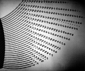
To make the comparisons between simulations and experiments conveniently, we show the spiralling jet in a space time plot in figure 5 (without actuation) and figure 6 (with actuation) by stitching consecutive time images together. This also allows us to inspect the motion of the droplets after the pinch-off event, such as capillary oscillations and rotation. The time difference between instants is  $\Delta t = 0.8$ ms, during which the orifice rotates ${\rm \pi} /150$ rad. By comparing figures 5 and 6 it is clear that jet actuation helps in achieving a regular jet breakup and reduces the fluctuation in the jet intact length. Also, the comparison of the drop size distributions in figures 5(c) and 6(c) reveal a narrower distribution around the mean projected drop area when the jet is actuated. Overall the agreement between the experiments and simulations is good. Figures 5 and 6 also allow for a qualitative comparison in terms of the late jet dynamics, formation of satellite drops and droplet motion after pinch-off.

Figure 5. Comparison between experiment and simulation for the natural (actuation-free) breakup case. (a) Experiment. (b) Simulation. (c) Comparison of the drop projected area normalized by the mean.

Figure 6. Comparison between experiment and simulation in the presence of actuation with  $\omega =0.9$. (a) Experiments with a piezoplate displacement of $6\ \mathrm {\mu } {\rm m}$. (b) Simulations with a velocity amplitude 0.5 %. (c) Comparison of the drop projected area normalized by the mean.
For the unperturbed jets, the intact length of the jet fluctuates at a higher standard deviation than their perturbed counterpart. The jets often emit filaments that are a few wavelengths long that fragment into droplets after separating from the main jet. Due to the thinning and stretching of the jet, the high-frequency perturbations that are initially stable and damped, may become unstable downstream. Therefore, a larger window of wavelengths is involved in the instability process as compared with the Rayleigh window for straight jets in the absence of external forces.
In the presence of jet actuation, the jet intact length fluctuations are suppressed and the jet regularly emits a filament that breaks up either at the forward/downstream end or the rear/upstream end. For straight jets, it is known that the location of the breakup within a single filament depends both on perturbation frequency and amplitude (Pimbley & Lee Reference Pimbley and Lee1977). If the breakup occurs at the forward end, the satellite drop merges with the main drop that is following it, within a distance of a few wavelengths. Within a narrow window of amplitudes at a given frequency, the breakup location shifts from the downstream end to the rear end, which is the desired regime for applications such as continuous ink jet printing as the satellite drop merges with the leading main drop (McIlroy & Harlen Reference McIlroy and Harlen2019). The main mechanism of merging is the momentum transfer during the finite time between the two successive pinch-off events, also known as the satellite interaction time (Pimbley & Lee Reference Pimbley and Lee1977). In our simulations and experiments, the typical merging length relative to jet pinch-off in all cases is approximately 2–3 wavelengths. The proportion of the main and satellite droplet volumes are given in figure 7. The volumes are normalized with the jet volume over one perturbation wavelength at the nozzle exit, which is conserved under wavelength stretching downstream due to mass conservation. At a given frequency, the perturbation amplitude determines where the droplets are formed, i.e. lower amplitudes result in droplets formed further downstream. The proportion of the volumes of the main and satellite droplets converge as they are formed further downstream. For a nozzle frequency of  $\omega =1.2$, which is initially outside of the Rayleigh window, one can see a larger variation in the drop volume and location. This is attributed to the fact that the unstable frequencies of the white noise gain enough to interfere with the imposed finite-amplitude perturbation. Therefore, the jet volume enclosed by the imposed perturbation wavelength at nozzle exit becomes irrelevant and one can see the droplet volumes are exceeding the volume expected from the imposed perturbation.

Figure 7. Volumes of the main and satellite droplets obtained from the simulations as a function of their location of first appearance. For each frequency, three points are shown corresponding to different perturbation amplitudes (drops are formed further downstream for smaller amplitudes).
The fact that the droplets stay in the base jet trajectory in the experiments (see figure 6) verifies that it is a good approximation to assume that the jet trajectory is steady in the rotating frame and to separate the calculation of the base flow and the drop formation. After the pinch-off, the droplets travel in a straight line with respect to the stationary frame, preserving their linear momentum.
The satellite interaction time leads to another phenomenon in the context of spiralling jets. With straight jets, the momentum transfer is always in the direction of the flow and the satellite drop is either sped up or slowed down depending on the location of the first pinch-off (forward or rear). When the spiralling jets are captured in the stationary frame (figure 6), one can observe that the capillary oscillation of the droplets is superposed with a rotation around the principal axis. The curved nature of the trajectory results in slight variation of the tangential and the normal vectors from the front end to the rear end of the droplets, which leads to a moment around the principal axis and breaks the symmetry of the detached drop around the tangential direction. The locality of the forces along the flow direction imposes a moment during the satellite interaction time, causing the drop oscillations to be 3-D in nature.
As the perturbations grow and the amplitude becomes finite, the shape deformations of the jet are sufficiently large where the dynamics enter a nonlinear regime. The formation of the main and satellite droplets is a nonlinear phenomenon by nature. The evolution of the velocity perturbations deviates from its linear counterpart (i.e. normal mode), shown in figure 8 for  $\omega =0.9$, as the satellite droplets begin to form. It manifests itself as the fluctuations take the form of triangular waves starting from the sinusoidal. On the other hand the nonlinear growth rate is in agreement with the linear estimation until very close to the breakup, which is partly due to the fact that the studied case is close to the inviscid limit, where the time scale for axial momentum diffusion is large compared with the inertio-capillary time scale during the early stage of the growth. In other words, the jet is sufficiently deformed only very close to the breakup for viscosity to play a role.

Figure 8. Comparison of the linear and nonlinear evolution of the velocity perturbations for  $\omega = 0.9$ at different velocity perturbation amplitudes at the nozzle, with decreasing strength from top to the bottom. Here $t_b$ refers to the instant of jet breakup. The dotted lines represent the envelope of the velocity perturbations computed from the linear model detailed in § 5.
5. Analogy with gravity-driven straight jets: approximate base flow solutions, linear stability and self-similarity
The agreement between the experiments and simulations demonstrates the validity of modelling spiralling jets as quasi-straight and slender jets with locally varying pseudo forces provided that epsilon is sufficiently small. These forces, and the variation thereof, can be computed from the base trajectory of the jet as discussed in § 3.2. Once the base flow of the jet and the variation of the body forces have been accounted for, one can use these to study the stability of this flow to perturbations. In this section we will linearize the slender-jet model for a linear spatial stability analysis of the flow to infinitesimally small perturbations imposed at the nozzle exit. We will show that this analysis provides insight in the dynamics underlying jet breakup and in the scaling behaviour for the spatial growth rate and jet breakup.
To study how perturbations evolve along the jet, one needs to pay attention to the disparate length scales present in this problem. In § 3.2 where the base flow and the trajectory was calculated in the limit  $\epsilon \rightarrow 0$, all lengths are expressed in terms of the rotating arm $L$ and the base flow equations represent the jet as a ‘string’ whose thickness is $\textit {O}(\epsilon L)$. When we consider capillary waves along the jet, their wavelengths are of the same order as the jet radius so their growth should be expressed along $s/(\epsilon L)$, i.e. in units of jet radius instead of the rotating arm. Similarly, while the advective scale of the base flow is $t_{\textit {adv}}=L/U_0$, the relevant advective time for the perturbations is $R_0/U_0 = t_{\textit {adv}}/\epsilon$. In what follows, we will express all the lengths in terms of the nozzle radius and the length of the rotating arm $L$ will only appear in the expression of the body forces. Furthermore, we introduce an effective gravity $g_e\sim \textit {O}(\varOmega ^2L+g)$ that measures the combined effect of rotational and gravitational forces. Using this, we define the effective capillary length as $l_c = \sqrt {\gamma /\rho g_e}$ and an effective Bond number ${\textit {Bo}}_e=(R_0/l_c)^2=\rho g_e R_0^2/\gamma$. In terms of (We, Rb, Fr) given in table 1, the latter can be expressed as
 \begin{equation} {\textit{Bo}}_e({\textit{We}},{\textit{Fr}},{\textit{Rb}}) = {\textit{We}}\left(\frac{\epsilon}{{\textit{Rb}}^2}+\frac{\epsilon}{{\textit{Fr}}^2}\right). \end{equation}
 Using (5.1), one could follow the same line of gain analysis developed for straight jets in Le Dizès & Villermaux (Reference Le Dizès and Villermaux2017). For the given experimental case with the non-dimensional numbers presented in table 1, the variation of the body forces along the jet is minor; see figure 3(c). The centrifugal forces are very close to their nozzle value throughout the entire jet and gravitational forces, which would make the jet travel in the  $Z$ direction and cause torsion, are an order of magnitude smaller than the centrifugal forces. In this case, the spiralling jet thus behaves like a gravity-driven straight jet with the gravitational acceleration replaced by the initial centrifugal acceleration at the nozzle exit, namely, $U(dU/ds) = {\textit {Bo}}_e/{\textit {We}}$, as the viscous and curvature effects decay rapidly after the nozzle exit. One thus has
 $$\begin{gather} U(s) = \sqrt{\frac{2{\textit{Bo}}_e}{{\textit{We}}}s+1}, \end{gather}$$
 $$\begin{gather}R(s) = \left(\frac{2{\textit{Bo}}_e}{{\textit{We}}}s+1\right)^{{-}1/4}. \end{gather}$$
A comparison between the ‘free-fall’ solution (5.2) and the solution of the base flow equations (3.20) is given in figure 9.

This assumption can be made a priori if  ${\textit {We}}\gg {\textit {Bo}}_e$ for ${\textit {We}}$ large enough to stay in the jetting regime (Clanet & Lasheras Reference Clanet and Lasheras1999). The arc length $s$ can be recast as a slowly varying dimension
 \begin{equation} \xi = \frac{s}{s_0}+1, \quad s_0\,{\rm d}\xi = {\rm d}s, \end{equation}
for large  $s_0$, where $s_0 = {\textit {We}}/2{\textit {Bo}}_e$ is the variation scale (Le Dizès & Villermaux Reference Le Dizès and Villermaux2017; Eggers & Villermaux Reference Eggers and Villermaux2008), such that (5.2) becomes
 $$\begin{gather} U(\xi) = \sqrt{\xi}, \end{gather}$$
 $$\begin{gather}R(\xi) = \xi^{{-}1/4}, \end{gather}$$
respectively.
We now consider perturbations to the base flow of the following form:
 \begin{equation} (\tilde{u},\tilde{R}) = (u(\xi),r(\xi)) \exp\left({{\rm i}\left(s_0\int_1^\xi k(\xi')\,{\rm d}\xi'- \omega t\right)}\right). \end{equation}
Here  $k = k_r + \text {i}k_i$ is the complex wavenumber, $k_r=2{\rm \pi} /\lambda$ is the real wavenumber with $\lambda$ the perturbation wavelength (normalised with $R_0$), $-k_i$ is the spatial growth rate and $\omega$ is the real perturbation frequency imposed at the nozzle. Plugging $U+\tilde {u}$ and $R+\tilde {R}$ into (3.21a)–(3.21c) and considering the terms linear in $(\tilde {u},\tilde {R})$ up to $\textit {O}(1/s_0)$ yields
 $$\begin{gather} \left(kU-\omega\right)r(\xi) + \frac{kR}{2}u(\xi) = \textit{O}\left(\frac{1}{s_0}\right), \end{gather}$$
 $$\begin{gather}\left(kU-\omega-\frac{3\text{i}k^2}{{\textit{Re}}}\right)u(\xi) + \frac{k}{R^2{\textit{We}}}\left(k^2 R^2 -1\right)r(\xi) = \textit{O}\left(\frac{1}{s_0}\right), \end{gather}$$
which is analogous to equation (2.16) in Le Dizès & Villermaux (Reference Le Dizès and Villermaux2017). This approach is also known as the WKBJ (Wentzel–Kramers–Brillouin–Jeffreys) method (Bender & Orszag Reference Bender and Orszag1978), a perturbation method using expansions over the small parameter  $1/s_0$ in this case. This approach is well utilized and tested in Javadi et al. (Reference Javadi, Eggers, Bonn, Habibi and Ribe2013) and Le Dizès & Villermaux (Reference Le Dizès and Villermaux2017). The variations of the amplitudes $(u(\xi ),r(\xi ))$ and the base states only show up at higher orders, which means for large $s_0$ (i.e. ${\textit {We}}\gg {\textit {Bo}}_e$), the length scale of base flow variations are small compared with the perturbation wavelength. The dispersion relation is found from the non-trivial solution of (5.6),
 \begin{equation} \frac{k^2}{2R {\textit{We}}}\left(k^2 R^2 -1\right) - \left(kU-\omega\right)^2 + \frac{3\text{i}k^2}{{\textit{Re}}}\left(kU-\omega\right) = 0. \end{equation}
 This equation governs the convective instability of a jet to infinitesimally small perturbations at the nozzle exit at a given frequency  $\omega$. Note that the dispersion relation (5.7) is identical to that for a straight jet in the absence of body forces, except that here $U$ and $R$ are the local values instead of the nozzle values.
The solution to the dispersion relation given in (5.7) is shown in figure 10. The local wavenumber,  $k_r$, is the real part of the solution to the complex equation and it is decreasing from its nozzle value due to the thinning of the jet, also known as wavelength stretching (Eggers & Villermaux Reference Eggers and Villermaux2008). Based on the nozzle values, the frequency that has the maximum growth rate at the nozzle is $\omega _{\textit {ini}}\approx 0.718$. But as the body forces stretch the perturbed filaments, their growth rate also changes locally which leads to different gains along the jet, shown in figure 11(a). So a net gain approach is preferable to study the most unstable frequencies (Javadi et al. Reference Javadi, Eggers, Bonn, Habibi and Ribe2013; Le Dizès & Villermaux Reference Le Dizès and Villermaux2017). The local gain along the jet is then expressed as
 \begin{equation} G(\xi) = e^{S(\xi)}, \quad S(\xi) = s_0\int_1^\xi -k_i(\xi')\,{\rm d}\xi', \end{equation}
where  $s_0 = {\textit {We}}/2{\textit {Bo}}_e \sim 0.5\lvert \,{\rm d}U/{\rm d}s\rvert _0^{-1}/(R_0/U_0)$ can be interpreted as the ratio of the initial stretching time to the initial advective time.

Figure 10. The local wavenumber ( $k_r R_0$) and spatial growth rate ( $-k_i R_0$) along the jet. The dotted line indicates the upper boundary of the local Rayleigh window of unstable perturbations.

Figure 11. (a) Integrated gain for different frequencies of perturbation at the nozzle. The dashed vertical line indicates the location  $\xi =2.35$ that corresponds to the location of the mean jet intact length obtained from the experiments in the absence of imposed perturbations, also given in table 2. (b) The location to reach the gain necessary for breakup versus the frequency of perturbation at the nozzle.
Figure 11(a) shows the gain along the jet at different frequencies and for infinitesimal amplitude, based on (5.8a,b). The disturbances start to gain only when their local wavelength enters the Rayleigh window, which is indicated by the dotted line in figure 10. Quantification of the infinitesimal disturbances is a difficult practice both experimentally and numerically. When the gain reaches a sufficiently high value, which is assumed to be  $G\approx e^7$ in Le Dizès & Villermaux (Reference Le Dizès and Villermaux2017), the transition to breakup occurs. The location of the transition $\xi _t$ for different values of threshold gain is given in figure 11(b). For our experimental case with the parameters given in table 1, the assumed transition gain of $S_t\approx 7$ agrees well with the average natural breakup length for the unperturbed case of our experiments that is around 95 times the radius of the jet; see table 2. For the choice of $S_t\approx 7$, the frequency that gains the fastest is around $\omega \approx 0.9$.
Furthermore, self-similarity can be deduced from the dispersion relation. We will first decompose the solution of the complex equation (5.7) as
 $$\begin{gather} k_rR(\xi) = \frac{\omega R}{U}= \omega\xi^{{-}3/4}, \end{gather}$$
 $$\begin{gather}-k_iR(\xi) = q\left(k_rR,{\textit{Oh}}\right){\textit{We}}_l^{{-}1/2} = q\left(\omega \xi^{{-}3/4},{\textit{Oh}}\right){\textit{We}}^{{-}1/2}\xi^{{-}3/8}, \end{gather}$$
where  $q$ is a non-dimensional function of the local wavenumber, the perturbation frequency and the Ohnesorge number, and ${\textit {We}}_l = We\xi ^{3/4}$ is the local Weber number obtained by using the base flow solutions (5.4). Looking into the convective behaviour of the perturbations of $\omega >1$, one can see that the initial wavelength of these perturbations are shorter than the lower boundary of the Rayleigh window (i.e. $k_r(\xi )R\leq 1$ as shown with a dashed curve in figure 10), so these perturbations do not gain (or even damped with higher viscosity) until the wavelength is stretched enough to enter the Rayleigh window. This motivates us to do another rescaling on the flow direction, $\xi$, as
 \begin{equation} \theta = \xi\omega^{{-}4/3}, \end{equation}
such that  $k_rR(\theta )=\theta$ and instabilities grow for $\theta >1$. From here, we can express (5.9) explicitly in terms of $\theta$ using the base flow solutions (5.4),
 $$\begin{gather} k_r\omega^{{-}1/3} = \theta^{{-}1/2}, \end{gather}$$
 $$\begin{gather}-k_i\omega^{1/6}{\textit{We}}^{1/2} = q\left(\theta^{{-}3/4},{\textit{Oh}}\right)\theta^{{-}1/8}=p(\theta,{\textit{Oh}}), \end{gather}$$
where  $k_r$ and $k_i$ are now scaled with parameters defined at the nozzle exit. Using these rescaled solutions, we can collapse the curves given in figure 10 onto a single curve, which is shown in figure 12(a). We can also write the integral for the gain $S(\xi )$ given in (5.8a,b) in terms of an integral over the similarity variable $\theta$ using (5.11b),
 \begin{equation} S(\theta) = \frac{s_0\omega^{7/6}}{\sqrt{{\textit{We}}}}\int_1^\theta p(\theta',{\textit{Oh}})\,{\rm d}\theta'. \end{equation}
Figure 12. (a) Rescaled curves of the solution to the dispersion relation given in (5.7). (b) The gain associated with the rescaled curve.
This is plotted in figure 12(b) for different values of  $\omega$. For a threshold gain of $S_t\approx 7$, we can then deduce the rescaled threshold distance for jet breakup, $\theta _{t}$, numerically from (5.12). This is shown in figure 13(a). In figure 13(b) the threshold distance, $\xi _t = \theta _t\omega ^{4/3}$, and the wavelength at breakup calculated as $\lambda (\xi _t) = ({2{\rm \pi} }/{\omega })\xi _t^{1/2}$ are shown. The prefactor $s_0/\sqrt {{\textit {We}}}\sim 0.5\lvert \, {\rm d}U/{\rm d}s\rvert _0^{-1}/\sqrt {\rho R_0^3/\gamma }$ in (5.12) can be interpreted as the ratio of the initial stretching time to the initial inertio-capillary time.


As nonlinear effects present in the experiments are a priori excluded from the linear stability analysis, a direct quantitative comparison between the linear stability predictions and the experiments or the nonlinear slender-jet model would be flawed. Nevertheless, we made a quantitative comparison of the linear and nonlinear predictions for the evolution of the perturbations for the non-dimensional numbers given in table 1. To that end, we performed a small study where we compare the results from linear stability analysis with the nonlinear slender-jet model for two different perturbation amplitudes and a range of frequencies.
Results for the jet breakup length are given in figure 14 where the breakup length  $L_b$ is normalized by the minimum breakup length, $L_{b,min}$. One can see that although the value of the most unstable wavelength does agree between the linear and nonlinear predictions, the behaviour at other wavelengths differs significantly. At high frequencies (i.e. short wavelengths) and $\varepsilon _v = 1\,\%$, the nonlinear prediction for the jet breakup length does follow the $\omega ^{4/3}$ scaling, though slightly underestimating the breakup length. However, at low frequencies (i.e. long wavelengths) there is a significant overestimation of the breakup length by the linear analysis, as for $\omega \rightarrow 0$, the perturbation wavelengths become eventually large enough to be comparable to the streamwise variation scale of the base flow. To correct for this, it would be necessary to include higher-order terms in (5.6), starting with terms up to $O(1/s_0^2)$ and increasing the order for smaller $\omega$. In our study the focus is on the frequencies that are in the vicinity of the most unstable frequencies, corresponding to the larger frequencies and smaller perturbation wavelengths for which the local plane-wave approximation underlying (5.6) is valid.

Figure 14. Comparison of the breakup length from linear stability theory and from nonlinear simulations for two different velocity fluctuation amplitudes,  $\varepsilon _v$, as a function of the imposed perturbation frequency. To ease the comparison, the breakup length has been normalised with the minimum breakup length at the most unstable frequency. Values for $L_{b,min}$ are 91 $R_0$ from the linear stability, and 90.6 $R_0$ and 52.7 $R_0$ from the nonlinear simulations for $\varepsilon _v = 0.1\,\%$ and $\varepsilon _v = 1\,\%$, respectively.
6. Conclusion
We studied the breakup of a spiralling jet using experiments, simulations based on a slender-jet model and a spatial linear stability analysis. The good agreement between the experiments and simulations validates our ansatz that the spiralling jets can be approximated as quasi-straight jets with locally varying body forces given that the cross-sectional scale of the jet (of the order of the jet radius,  $R_0$) is much smaller than the longitudinal scale at which the base flow varies (of the order of $L$). The locally varying body forces are the longitudinal projections of the centrifugal and gravity forces along the jet. For the given set of non-dimensional parameters studied in our experiments, these longitudinal projections can be approximated by a constant effective gravity, and the base flow solution can be treated as a freely falling jet by defining an effective Bond number. The effect of the wavelength stretching manifests itself as a reduction in the inertio-capillary time scale along the jet due to thinning by the action of the effective gravity (i.e. the longitudinal projections of the centrifugal and gravity forces). Self-similar solutions for the convective linear stability have also been derived, from which a simple approximation can be derived for the jet breakup length. Despite the number of assumptions needed to proceed with this simplified approach, they are valid and relevant in many processes, such as prilling of fertilizers, where the working liquids (e.g. molten urea) have low viscosities.
Funding
This work has been financially supported by Machinefabriek Kreber BV under a TU Delft/Kreber Research Agreement.
Declaration of interests
The authors report no conflict of interest.
Appendix A. Relative effects of the white noise and harmonic components of velocity perturbation
In this appendix we assess the effect of varying the strength of the imposed white noise perturbations at the nozzle exit on jet breakup. In figure 15 the Fourier transforms of the nozzle exit velocity are given. One can see that for amplitudes greater than 0.1 %, the harmonic component is the main perturbation mechanism. The other frequency components imposed by the white noise would influence the time series of the instantaneous jet intact length.

Figure 15. Frequency spectrum of the nozzle velocity  $u(0,t)$ with respect to different amplitudes for the harmonic component and the noise component. The frequency of the harmonic component is $\omega =0.9$.
Figure 16 shows the mean jet intact length with respect to the amplitude of the imposed harmonic component at different levels of white noise intensity. In the absence of the harmonic component, one can see that the fluctuations of the intact length are much stronger. This is partly due to the fact that there is a wider window of unstable wavelengths because of the streamwise component of the body force. The wavelengths that are initially not long enough and, thus, stable will eventually get stretched and fall into the instability window. When the amplitude of the harmonic component is weak, the frequencies within the white noise have more time to be stretched and interfere with the instability. When the amplitude of the harmonic component is strong, harmonic perturbation will dominate the dynamics, which can also be seen by narrowing of the errorbars at high amplitudes in figure 16.

Figure 16. Variation of the jet intact length with respect to different strengths of harmonic and the white noise components. Here, the frequency of the harmonic component is  $\omega =0.9$ and $\Delta t$ is the adaptive computational time step. The errorbars are one standard deviation of the intact length.
Appendix B. Obtaining  $p(\theta )$

We use the fact that the convective growth rate can be expressed in terms of temporal growth rate given that we are above the critical wavenumber, i.e.
 \begin{equation} k_i(\xi) = \frac{\omega_{\textit{i,temp}}(\xi)}{t_{IC}(\xi)U(\xi)}. \end{equation}
The temporal growth rate can be deduced from the classical Rayleigh–Plateau instability as
 \begin{equation} \omega_{\textit{i,temp}}(\xi) = \frac{k}{\sqrt{2}}\sqrt{1-k^2+\frac{9{\textit{Oh}}^2 k^2}{2}}-\frac{3{\textit{Oh}} k^2}{2}, \end{equation}
where  $k$ is the local real wavenumber. The local values of $k$,
$k$,  ${\textit {Oh}}$, $t_{IC}$ and $U$ are as follows:
 $$\begin{gather} k(\xi) = \omega\xi^{{-}3/4}, \end{gather}$$
 $$\begin{gather}{\textit{Oh}}_l(\xi) = {\textit{Oh}}\xi^{1/8}, \end{gather}$$
 $$\begin{gather}t_{IC}(\xi) = \sqrt{{\textit{We}}}\xi^{{-}3/8}, \end{gather}$$
 $$\begin{gather}U(\xi) = \xi^{{-}1/2}. \end{gather}$$
 When we substitute these into (B2) and use (B1) to evaluate  $k_i(\xi )$, we end up with
 \begin{equation} k_i(\xi) = \frac{\omega}{\sqrt{2{\textit{We}}}}\xi^{{-}7/8}\left(\sqrt{1-\omega^2\xi^{{-}3/2}+\frac{9{\textit{Oh}}^2\omega^2}{2}\xi^{{-}5/4}}-\frac{3{\textit{Oh}}\omega}{\sqrt{2}}\xi^{{-}5/8}\right). \end{equation}
 Using the transformations given in (5.10) and (5.11b), we finally obtain  $p(\theta )$ explicitly as
 \begin{equation} p(\theta) = \sqrt{\frac{1-\theta^{{-}3/2}}{2}+\frac{9{\textit{Oh}}^2\omega^{1/3}}{4}\theta^{{-}5/4}}-\frac{3{\textit{Oh}}\omega^{1/6}}{2}\theta^{{-}5/8}. \end{equation}
 When  $p(\theta )$ can be explicitly integrated, (5.12) would then give an explicit equation to solve for $\theta _{t}$,
 \begin{equation} S_t = \frac{s_0\omega^{7/6}}{\sqrt{{\textit{We}}}}\left[P(\theta_t)-P(1)\right], \end{equation}
where  $S_t\approx 7$ and $P(\theta )=\int p(\theta )\,{\rm d}\theta$.
Appendix C. Christoffel symbols, expressions in local and Frenet frames
Here we provide the intermediate expressions to define the local coordinate system and the terms in the governing equations.
Using (3.9), one can represent the local base vectors in terms of the Frenet frame as follows:
 \begin{equation} \left[{\begin{array}{@{}c@{}} \boldsymbol{T} \\ \boldsymbol{N} \\ \boldsymbol{B} \end{array}}\right] = \left[{\begin{array}{@{}ccc@{}} \dfrac{1}{1-r\kappa\cos{\phi}} & 0 & \dfrac{-\tau}{1-r\kappa\cos{\phi}} \\ 0 & \cos{\phi} & -\dfrac{\sin{\phi}}{r} \\ 0 & \sin{\phi} & \dfrac{\cos{\phi}}{r} \end{array}}\right]\left[{\begin{array}{@{}c@{}} \boldsymbol{e}_1 \\ \boldsymbol{e}_2 \\ \boldsymbol{e}_3 \end{array}}\right]. \end{equation}
 As mentioned in § 3.1 and seen in (3.11), the local base vectors are not necessarily unit. The magnitudes of the local base vectors should be used in order to express the physical velocity  $\boldsymbol {u} = (u_s,u_r,u_{\phi })$ vector from the contravariant vector $\boldsymbol {v} = (v^1,v^2,v^3)$ as follows:
 \begin{align} u_s = v^1|\boldsymbol{e}_1| = v^1\sqrt{(1-r\kappa\cos{\phi})^2 + (r\tau)^2}, \quad u_r = v^2|\boldsymbol{e}_2| = v^2, \quad u_{\phi} = v^3|\boldsymbol{e}_3| = v^3r. \end{align}
The Christoffel symbols of the second kind, whose compact form is given in (3.14), can be written explicitly as follows:
 \begin{equation} \left. \begin{gathered} \displaystyle\varGamma_{11}^1 = \dfrac{r}{1-r\kappa\cos{\phi}} \left( \kappa \tau \sin{\phi} - \cos{\phi} \dfrac{{\rm d}\kappa}{{\rm d}s} \right),\\ \displaystyle \varGamma_{11}^2 = \left(1-r\kappa\cos{\phi}\right)\kappa\cos{\phi}-r\tau^2,\\ \displaystyle \varGamma_{11}^3 = \dfrac{r\tau}{1-r\kappa\cos{\phi}} \left(\cos{\phi} \dfrac{{\rm d}\kappa}{{\rm d}s} - \kappa \tau \sin{\phi} \right)-\left(1-r\kappa\cos{\phi}\right)\dfrac{\kappa\sin{\phi}}{r}+\dfrac{{\rm d}\tau}{{\rm d}s},\\ \displaystyle \varGamma_{22}^1=\varGamma_{22}^2=\varGamma_{22}^3=0, \quad \varGamma_{23}^1=\varGamma_{32}^1=0, \quad \varGamma_{23}^2=\varGamma_{32}^2=0,\\ \displaystyle \varGamma_{33}^1=\varGamma_{33}^3=0, \quad \varGamma_{33}^2 ={-}r, \quad \varGamma_{23}^3=\varGamma_{32}^3=\dfrac{1}{r},\\ \displaystyle \varGamma_{12}^1=\varGamma_{21}^1={-}\dfrac{\kappa\cos{\phi}}{1-r\kappa\cos{\phi}}, \quad \varGamma_{13}^1=\varGamma_{31}^1=\dfrac{r\kappa\sin{\phi}}{1-r\kappa\cos{\phi}},\\ \displaystyle \varGamma_{12}^2=\varGamma_{21}^2=0, \quad \varGamma_{13}^2=\varGamma_{31}^2={-}r\tau,\\ \displaystyle \varGamma_{12}^3=\varGamma_{21}^3=\dfrac{\kappa\tau\cos{\phi}}{1-r\kappa\cos{\phi}}+\dfrac{\tau}{r}, \quad \varGamma_{13}^3=\varGamma_{31}^3={-}\dfrac{r\kappa\tau\sin{\phi}}{1-r\kappa\cos{\phi}}. \end{gathered} \right\} \end{equation}
The covariant terms in the conservation equations can be written in the general coordinates as follows:
 $$\begin{gather} \dfrac{{\rm D}\boldsymbol{v}}{{\rm D}t} = \left(\dfrac{\partial v^i}{\partial t}+ v^j\left(\dfrac{\partial v^i}{\partial s^j}+v^k\varGamma_{jk}^i\right)\right)\boldsymbol{e}_i, \end{gather}$$
 $$\begin{gather}-\boldsymbol{\nabla} p = g^{ij}\dfrac{\partial p}{\partial s^j}\boldsymbol{e}_i, \end{gather}$$
 $$\begin{gather}\left(2\boldsymbol{\mathsf{D}}\right)^{ij} = g^{kj}\left(\dfrac{\partial v^i}{\partial s^k}+\varGamma_{kl}^i v^l\right)+g^{ki}\left(\dfrac{\partial v^j}{\partial s^k}+\varGamma_{kl}^j v^l\right), \end{gather}$$
 $$\begin{gather}\dfrac{1}{{\textit{Re}}}\boldsymbol{\nabla}\boldsymbol{\cdot}\left(2\boldsymbol{\mathsf{D}}\right) = \dfrac{1}{{\textit{Re}}}\left(\dfrac{1}{\sqrt{\varDelta}}\dfrac{\partial}{\partial s^j}\left(\sqrt{\varDelta}(2\boldsymbol{\mathsf{D}})^{ij}\right)+\varGamma_{jk}^{i}\left(2\boldsymbol{\mathsf{D}}\right)^{ij}\right)\boldsymbol{e}_i. \end{gather}$$
One can then use the metric tensor (and its inverse) and the Christoffel symbols listed in (3.11), (3.12) and (C3) to compute the terms given above in ((C4a)–(C4d)). To compute the projections in the Frenet frame one can use the transformation given in (C1).
Appendix D. Benchmark for the slender-jet simulation
We validate our slender-jet model that includes the longitudinal projections of the computed body forces with the results of the arbitrary Lagrangian–Eulerian simulation presented in Li et al. (Reference Li, Sisoev and Shikhmurzaev2019). Their approach considers a boundary (a free parameter) between linear–nonlinear evolution of the perturbation and this boundary is validated by convergence of the breakup length over different choices of the linear–nonlinear boundary. In figure 17, we show the case where this boundary is directly set at the nozzle exit, corresponding to the results shown in figure 3 of Li et al. (Reference Li, Sisoev and Shikhmurzaev2019).

Figure 17. Jet shapes from our slender-jet model for the parameters  ${\textit {We}}=10$, ${\textit {Fr}}=5$, ${\textit {Rb}}=1$, ${\textit {Re}}=50$ and $\epsilon =0.0172$, for one droplet generation cycle. Plots ( $a-d$) correspond to $t$ = 0, 1.9, 3.9, 5.8; ( $e-h$) correspond to $t$ = 7.6, 7.9, 8.1, 8.5, where $t$ is measured from the beginning of the cycle. The frequency and the amplitude of the radius perturbation are $\omega =0.736$ and $\varepsilon _R = 0.04$. The results are in agreement with the results of Li et al. (Reference Li, Sisoev and Shikhmurzaev2019), figure 3.
The pinch-off location of the main drop in both our simulations and in Li et al. (Reference Li, Sisoev and Shikhmurzaev2019) is 46–48 times the radius of the jet and the period of the drop generation cycle is 8.5 in units of  $R_0/U_0$, which corresponds to the period of the nozzle excitation $2{\rm \pi} /\omega$.


 Open access