


1. Introduction
The majority of temperate ice masses in the southern hemisphere can be found in Patagonia, between 46.5°S and 51.5°S, home to dynamic calving glaciers (Aniya and others, Reference Aniya, Sato, Naruse, Skvarca and Casassa1997). The northern and southern Patagonian icefields are the two main ice masses in the region, covering ~3,700 km2 and ~12,000 km2, respectively (Meier and others, Reference Meier, Grießinger, Hochreuther and Braun2018). They are losing ice mass at one of the highest rates in the world (Hugonnet and others, Reference Hugonnet2021). This is because lake- and ocean-terminating glaciers dominate 80% of the outlet glaciers (Aniya and others, Reference Aniya, Sato, Naruse, Skvarca and Casassa1997). These calving glaciers lose ice mass not only at the ice surface but also at their terminus through frontal ablation, consisting of iceberg calving and subaqueous melting (e.g. Truffer and Motyka, Reference Truffer and Motyka2016). The number of lake-terminating glaciers in both icefields accounts for more than 70% of calving glaciers and constitutes 74% of the mass loss from the icefields (e.g. Minowa and others, Reference Minowa, Schaefer, Sugiyama, Sakakibara and Skvarca2021). These lake-terminating glaciers in Patagonia flow at a high rate ranging from several hundred metres to kilometres per year (Sakakibara and Sugiyama, Reference Sakakibara and Sugiyama2014; Mouginot and Rignot, Reference Mouginot and Rignot2015), and have shown heterogeneous fluctuation over the last few decades (e.g. Aniya and others, Reference Aniya, Sato, Naruse, Skvarca and Casassa1997; Sakakibara and Sugiyama, Reference Sakakibara and Sugiyama2014). Therefore, understanding the mechanisms of ice mass change in lake-terminating glaciers is important for interpreting the current and future mass changes of Patagonian glaciers.
Ice dynamics play a major role in the mass change of calving glaciers (e.g. Meier and Post, Reference Meier and Post1987; O'Neel and others, Reference O'Neel, Pfeffer, Krimmel and Meier2005; Bevan and others, Reference Bevan, Luckman and Murray2012; Felikson and others, Reference Felikson2017). This is because the ice flow at the lower reach of a calving glacier is primarily determined by basal sliding, which relates to driving stress and inversely relates to effective pressure (Sugiyama and others, Reference Sugiyama2011; Doyle and others, Reference Doyle2018; Christmann and others, Reference Christmann2021). The driving stress is controlled by ice thickness and surface slope. The effective pressure is defined as the difference between overburden ice pressure and hydraulic subglacial water pressure. The greatest ice flow is found near the terminus of a calving glacier, where effective pressure is usually small. Thus, the acceleration of ice flow at the terminus extends and thins the glacier, i.e. causes dynamic thinning, which steepens the ice surface and further accelerates the ice flow by increasing driving stress and reducing effective pressure (Benn and others, Reference Benn, Warren and Mottram2007). Ice flow acceleration causes more ice fracture and calving, resulting in ice front retreat. For example, Columbia Glacier in Prince William Sound has retreated by ~20 km since the 1980s accompanied by flow acceleration and thinning (O'Neel and others, Reference O'Neel, Pfeffer, Krimmel and Meier2005). The retreat was controlled by overdeepening basins (Meier and Post, Reference Meier and Post1987), often formed by glacial erosion (Cook and Swift, Reference Cook and Swift2012). This is because effective pressure decreases substantially when glaciers get close to floating by decreasing basal drag and causing ice flow acceleration (Kamb and others, Reference Kamb1994; Meier and others, Reference Meier1994; O'Neel and others, Reference O'Neel, Pfeffer, Krimmel and Meier2005). Once the ice front retreats into a deeper basin, instability takes place by losing buttressing effect, increasing ice flow and enhancing calving rate (Benn and others, Reference Benn, Warren and Mottram2007). Moreover, modelling (Nick and others, Reference Nick, Vieli, Howat and Joughin2009; Enderlin and Howat, Reference Enderlin and Howat2013; Frank and others, Reference Frank, Åkesson, de Fleurian, Morlighem and Nisancioglu2022) and theoretical studies (e.g. Weertman, Reference Weertman1974; Pfeffer, Reference Pfeffer2007) have also strongly suggested the topography influence on the dynamic calving glacier's retreat. Therefore, knowing the ice flow acceleration and iceberg calving mechanisms, and their relation to topography are essential to understand the rapid mass loss of calving glaciers (e.g. Benn and others, Reference Benn, Warren and Mottram2007; Truffer and Motyka, Reference Truffer and Motyka2016; Benn and others, Reference Benn, Cowton, Todd and Luckman2017; Felikson and others, Reference Felikson2017; Catania and others, Reference Catania2018).
Buoyancy force plays an important role in the increase in ice speed and iceberg calving (Meier and Post, Reference Meier and Post1987; O'Neel and others, Reference O'Neel, Pfeffer, Krimmel and Meier2005; Benn and others, Reference Benn, Warren and Mottram2007; Stearns and Van der Veen, Reference Stearns and Van der Veen2018). Because the calving front of an ocean-terminating glacier is often highly fractured and not strong enough to accommodate buoyancy force, it causes very large calving events, as has been observed in the ocean-terminating glaciers in Alaska (Walter and others, Reference Walter2010) and in Greenland (Amundson and others, Reference Amundson2008; James and others, Reference James, Murray, Selmes, Scharrer and O'Leary2014; Murray and others, Reference Murray2015). It appears that the recent thinning of calving glaciers results in the front being more vulnerable to buoyancy force, which triggers large-scale calving in Greenland (van Dongen, Reference van Dongen2021). Furthermore, large-scale calving can initiate flow acceleration by changing the force-balance near the terminus (Amundson and others, Reference Amundson, Truffer and Zwinger2022; Ultee and others, Reference Ultee, Felikson, Minchew, Stearns and Riel2022). It has also been reported that the importance of buoyancy force for glacier calving on retreat in the lake-terminating glaciers. Several studies in Patagonia (Naruse and Skvarca, Reference Naruse and Skvarca2000; Warren and others, Reference Warren, Benn, Winchester and Harrison2001) and Alaska (Boyce and others, Reference Boyce, Motyka and Truffer2007) suggested that transiently floating tongues can form because the lake-terminating glaciers have fewer fractures (e.g. less flow speed, tidal flexure and low subaqueous melting). For just such a transient floating tongue at Glaciar Nef, Patagonia, Warren and others (Reference Warren, Benn, Winchester and Harrison2001) argued that buoyancy force acts on the tongue to cause tensile stress at the base of a glacier, resulting in a basal crevasse and catastrophic iceberg calving events. Boyce and others (Reference Boyce, Motyka and Truffer2007) reported that the floating ice front of Mendenhall Glacier, Alaska, lasted about two years before it calved due to a small increase in lake level (i.e. an increase in buoyancy force). More recently, a large-scale buoyancy-driven calving was documented at Glaciar Grey, a lake-terminating glacier in Patagonia (Sugiyama and others, Reference Sugiyama, Minowa and Schaefer2019). Therefore, knowing the floating condition near the ice front provides crucial information on how the buoyancy force influences the dynamic glacier retreat.
In lake-terminating glaciers in Patagonia, ice flow acceleration has been postulated to be the cause of the rapid retreat and thinning observed (e.g. Naruse and others, Reference Naruse, Skvarca and Takeuchi1997; Rignot and others, Reference Rignot, Rivera and Casassa2003; Sakakibara and others, Reference Sakakibara, Sugiyama, Sawagaki, Marinsek and Skvarca2013; Sakakibara and Sugiyama, Reference Sakakibara and Sugiyama2014; Mouginot and Rignot, Reference Mouginot and Rignot2015; Abdel Jaber and others, Reference Abdel Jaber, Rott, Floricioiu, Wuite and Miranda2019). These studies have also suggested that the bed topography near the terminus is essential for the observed rapid retreat. However, bedrock topography data near the terminus of calving glaciers is limited in Patagonia (Gourlet and others, Reference Gourlet, Rignot, Rivera and Casassa2016; Millan and others, Reference Millan2019). A field survey of lake geometry and a detailed comparison between glacier dynamics and geometry can provide insight into the mechanisms which accelerate ice flow. It can also increase our understanding about the importance of the rapid dynamic retreat for the glacier mass budget by increasing iceberg calving.
In this study, we present the lake topography measured near the terminus of four lake-terminating glaciers: O'Higgins, Viedma, Upsala and Tyndall glaciers. These glaciers are located on the eastern side of the southern Patagonian icefield ranging from 48.5°S and 51.5°S (Fig. 1). We analysed ice-front position, surface speed and surface elevation change between 2000 and 2021, using variable optical remote sensed imagery, which we compared with geometry near the termini. Particularly, we calculated the height above buoyancy near the ice front using bed topography and ice surface elevation to discuss how ice flow and calving change under near buoyant and buoyant conditions. Our study helps to understand the mechanisms of the rapid retreat and mass loss of lake-terminating glaciers in Patagonia.

Figure 1. (a) Satellite images showing the study area. Glacier basins in 2000 are indicated by black lines. Satellite images are taken by Sentinel-2A on March 3 2021, composed by sentinelflow (Seguinot, Reference Seguinot2020). Topographic maps of (b) O'Higgins, (c) Viedma, (d) Upsala and (e) Tyndall glaciers with 100 m contour intervals. The centreline of each glacier is indicated by white and red circles, dotted every 1 and 10 km, respectively, and starts from the head of the glacier towards down-glacier. Orange lines and green crosses indicate the place where the mean surface elevation and ice speed were obtained, respectively.
2. Study site
2.1 Glaciar O'Higgins
Glaciar O'Higgins is the fourth largest glacier in the southern Patagonian icefield, covering 762 km2 (De Angelis, Reference De Angelis2014). The surface elevation of the glacier ranges from 3,200 m at Volcán Lautaro to 252 m at O'Higgins/Lago San Martin (Fig. 1). The glacier width near the terminus is ~2.5 km (Fig. 1). Historical aerial photograph analysis shows that the glacier has experienced a rapid ice front retreat of approximately 15 km over almost a century since 1896 (Casassa and others, Reference Casassa, Brecher, Rivera and Aniya1997) when the ice front passed deep water ~800 m (Schaefer and others, Reference Schaefer, Casassa and Loriaux2011). After the rapid retreat, the retreat rate decreased to 36 m a−1 between 1984 and 2000 and to 17 m a−1 between 2000 and 2011 (Sakakibara and Sugiyama, Reference Sakakibara and Sugiyama2014). The ice flow speed in the lower ablation area shows it to have the fastest speed among the lake-terminating glaciers in Patagonia, probably due to the steep surface slope (Sakakibara and Sugiyama, Reference Sakakibara and Sugiyama2014; Mouginot and Rignot, Reference Mouginot and Rignot2015). Its speed was close to 5 km a−1 near the terminus in 1984, which decreased substantially down to 2 km a−1 in 2014 (Mouginot and Rignot, Reference Mouginot and Rignot2015). The ice volume change rate is −0.89 km3 a−1 between 2000 and 2012 and −0.85 km3 a−1 between 2012 and 2016 (Abdel Jaber and others, Reference Abdel Jaber, Rott, Floricioiu, Wuite and Miranda2019).
2.2 Glaciar Viedma
Glaciar Viedma is the second-largest glacier in the southern Patagonian icefield (De Angelis, Reference De Angelis2014), covering 974 km2 in area and shares its accumulation area with Pío XI, O'Higgins, Chico and Upsala glaciers (Fig. 1). The glacier flows into Lago Viedma (252 m a.s.l.) at a flow speed of ~1 km a−1 near the ~1.5 km wide terminus (Sakakibara and Sugiyama, Reference Sakakibara and Sugiyama2014). The retreat rate of the ice-front position was 30 m a−1 between 1984 and 2000 and 41 m a−1 between 2000 and 2011 (Sakakibara and Sugiyama, Reference Sakakibara and Sugiyama2014). Lake water depth was measured in the summer of 2012 and 2013 near the terminus of the glacier (Sugiyama and others, Reference Sugiyama2016). These measurements showed an increased water depth towards the ice front with a maximum depth of ~390 m close to the front. The ice volume change rate is −1.95 km3 a−1 between 2000 and 2012, which slightly increased to −2.3 km3 a−1 between 2012 and 2016 (Abdel Jaber and others, Reference Abdel Jaber, Rott, Floricioiu, Wuite and Miranda2019).
2.3 Glaciar Upsala
Glaciar Upsala is one of the most well-studied glaciers in the region. Fieldwork and remote sensing data revealed a rapid retreat (e.g. Warren and others, Reference Warren, Greene and Glasser1995b; Naruse and others, Reference Naruse, Skvarca and Takeuchi1997; Skvarca and Naruse, Reference Skvarca and Naruse1997; Skvarca and others, Reference Skvarca, De Angelis, Naruse, Warren and Aniya2002, Reference Skvarca, Raup and De Angelis2003; Muto and Furuya, Reference Muto and Furuya2013; Sakakibara and others, Reference Sakakibara, Sugiyama, Sawagaki, Marinsek and Skvarca2013; Mouginot and Rignot, Reference Mouginot and Rignot2015; Sakakibara, Reference Sakakibara2016; Abdel Jaber and others, Reference Abdel Jaber, Rott, Floricioiu, Wuite and Miranda2019). The glacier covers 835 km2 of the southern Patagonian icefield (De Angelis, Reference De Angelis2014) and flows into Brazo Upsala (177.5 m a.s.l.), a northwestern arm of Lago Argentino, at a rate of 2 km a−1 near the ~3 km wide terminus (Sakakibara and Sugiyama, Reference Sakakibara and Sugiyama2014). Early studies reported that rapid retreat occurred in the 90 s when the ice front retreated up to 700 m a−1 and ice thinning reached 11 m a−1 in the eastern half of the glacier (Skvarca and others, Reference Skvarca, Satow, Naruse and Leiva1995). It was suggested that the dynamic thinning caused the rapid retreat (Naruse and others, Reference Naruse, Skvarca and Takeuchi1997; Skvarca and others, Reference Skvarca, De Angelis, Naruse, Warren and Aniya2002). Another rapid retreat occurred in 2008, and the changes in ice-front position, surface elevation, and ice speed were documented by Sakakibara and others (Reference Sakakibara, Sugiyama, Sawagaki, Marinsek and Skvarca2013), who also reported that the glacier has retreated 2.9 km, accelerated 20–50% between 2008 and 2011 and the thinning rate reached 39 m a−1 between 2006 and 2010. Lake water topography over the region where the rapid retreat occurred was reported by Sugiyama and others (Reference Sugiyama2016) but has not yet been compared with the glacier fluctuation. The maximum depth along the Brazo Upsala arm ranged between 560 and 580 m. Due to this rapid retreat and acceleration, the volume change rate is the largest in Patagonia between 2000 and 2012 at −2.8 km3 a−1, which slightly decreased to −2.5 km3 a−1 between 2012 and 2016 (Abdel Jaber and others, Reference Abdel Jaber, Rott, Floricioiu, Wuite and Miranda2019).
2.4 Glaciar Tyndall
Glaciar Tyndall is located in the southernmost part of the southern Patagonian icefield (Fig. 1), covering 309 km2 of the icefield (De Angelis, Reference De Angelis2014). The glacier flows into Lago Geike (40 m a.s.l.), which is a small proglacial lake, compared with other lakes described above (Fig. 1a). The flow speed is about 500 m a−1 near the ~2 km wide terminus, which is also lower than at the other three glaciers. The glacier has shown continuous retreat and thinning over several decades (Naruse and others, Reference Naruse, Peña, Aniya and Inoue1987; Kadota and others, Reference Kadota, Naruse, Skvarca and Aniya1992; Nishida and others, Reference Nishida, Satow, Aniya, Casassa and Kadota1995; Rivera and Casassa, Reference Rivera and Casassa2004; Raymond and others, Reference Raymond2005; Sakakibara and Sugiyama, Reference Sakakibara and Sugiyama2014). For example, the retreat rate was 80 m a−1 between 1986 and 2000, and 135 m a−1 between 2000 and 2011, while no significant ice speed variation was reported during those periods (Sakakibara and Sugiyama, Reference Sakakibara and Sugiyama2014). A bathymetry survey of Lago Geike was performed in 2001 (Raymond and others, Reference Raymond2005). A traverse profile in the lake a few hundred metres from the ice front showed a U-shaped profile with a maximum depth of about 350 m (Fig. 4 in Raymond and others (Reference Raymond2005)). The ice volume change rate is −0.79 km3 a−1 between 2000 and 2012, which slightly decreased to −0.48 km3 a−1 between 2012 and 2016 (Abdel Jaber and others, Reference Abdel Jaber, Rott, Floricioiu, Wuite and Miranda2019).
3. Materials and methods
An overview of the available dataset used in this study is summarized in Figure 12.
3.1 Lake bathymetry
The water depth measurements were repeated in sections of glacier retreat at Lago Viedma and Brazo Upsala after previous measurements were taken in 1998 and 1999 (Skvarca and others, Reference Skvarca, De Angelis, Naruse, Warren and Aniya2002) and again in 2012, 2013 and 2014 (Sugiyama and others, Reference Sugiyama2016) (Fig. 2). Water depth was measured in January 2017, November 2018, November 2019 and June 2020 in Lago Viedma, and November 2019 and March 2020 in Brazo Upsala (Fig. 12). We also performed a water depth observation at Lago O'Higgins in February 2020 and Lago Geike in October 2019 (Figs 2 and 12). While water depth sounding was carried out with a kayak at Lago Geike due to a lack of regular boat operations, a small boat was used to conduct measurements in the other lakes. We used a depth sounder (Lowrance HDS-7) operated with an 80 kHz frequency-modulated transducer (Airmar B75M). The horizontal coordinates were obtained by a built-in single-frequency GPS. Water depth, horizontal coordinates and echograms were recorded every 1 sec. The uncertainty of the observed depth was estimated in the previous studies to be 5.7 m, or 3.7% of the observed depth by comparing the depth obtained using a water pressure sensor (Sugiyama and others, Reference Sugiyama2016, Reference Sugiyama2021), while the error in horizontal coordinates is expected to be several metres. To generate a bathymetry map, we compiled our observations with the early observations of the lake topography at Lago Viedma and Brazo Upsala (Skvarca and others, Reference Skvarca, De Angelis, Naruse, Warren and Aniya2002; Sugiyama and others, Reference Sugiyama2016). Finally, irregular depth datasets were interpolated into a 50 m grid matrix with a conventional natural neighbouring interpolation method (Watson, Reference Watson1999).
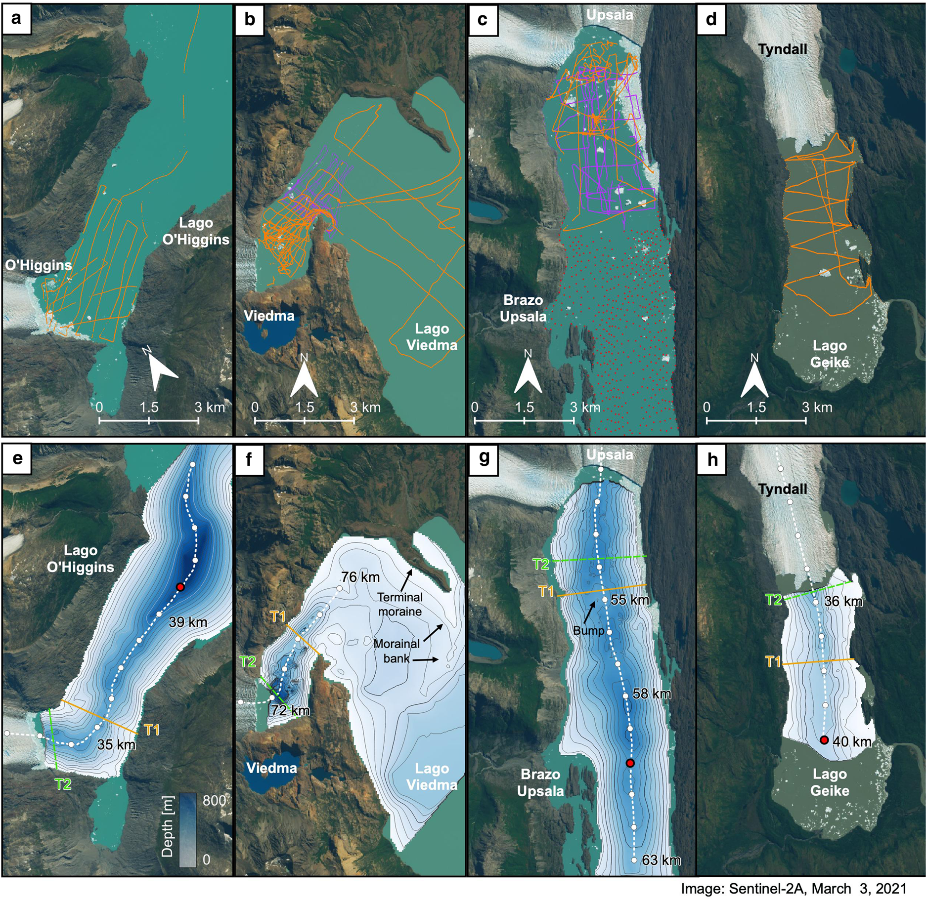
Figure 2. Orange lines indicate the survey lines of water depth in this study in front of (a) O'Higgins, (b) Viedma, (c) Upsala and (d) Tyndall glaciers. Purple lines and red dots indicate previous bathymetry observations by Sugiyama and others (Reference Sugiyama2016) and Skvarca and others (Reference Skvarca, De Angelis, Naruse, Warren and Aniya2002). Generated bathymetry map is indicated for (e) O'Higgins, (f) Viedma, (g) Upsala and (h) Tyndall glaciers. Water depth contour intervals are every 50 m. Two cross-sectional profiles were obtained along solid orange and dashed green lines denoted T1 and T2, chosen to cross the shallowest and the deepest parts of the lake, which have appeared after the recent glacier's retreat since 2000. The background satellite image was acquired by Sentinel-2A on March 3, 2021.
3.2 Ice front position, surface speed and surface elevation
We extended observations of the ice-front position, surface speed and surface elevation obtained in the previous studies (Sakakibara and Sugiyama, Reference Sakakibara and Sugiyama2014; Minowa and others, Reference Minowa, Schaefer, Sugiyama, Sakakibara and Skvarca2021). We analysed Landsat 8 images between 2019 and 2021 and Sentinel-2 images between 2016 and 2021. The ice-front position was manually delineated on a geographic information system using true-colour images (Fig. 12). The composite images generated by Landsat 8 and Sentinel-2 have 30 and 10 m resolutions, respectively. Combining the ice-front position mapped in the previous studies (Sakakibara and Sugiyama, Reference Sakakibara and Sugiyama2014; Minowa and others, Reference Minowa, Schaefer, Sugiyama, Sakakibara and Skvarca2021), our study covers variations in the ice-front position since the 1970s.
The optical images were also used to calculate the surface ice speed. For Landsat 8, we applied the feature-tracking method developed for analysing Landsat images in the previous study (Sakakibara and Sugiyama, Reference Sakakibara and Sugiyama2014). The programming code uses the orientation correlation method in the frequency domain to measure displacement (Haug and others, Reference Haug, Kääb and Skvarca2010; Heid and Kääb, Reference Heid and Kääb2012). For Sentinel-2 images, we applied the same method but with a different toolbox called ImGRAFT (Messerli and Grinsted, Reference Messerli and Grinsted2015). Temporal separation of the images was set to be between 16 and 60 days for Landsat 8 and between 10 to 60 days for Sentinel-2. Uncertainty in the ice speed measurement was analysed regarding co-registration errors, ambiguity in the cross-correlation peak and false correlation. The first two errors were accounted for by taking misfits between two images on bedrock areas, and the last error was evaluated for each grid (Sakakibara and Sugiyama, Reference Sakakibara and Sugiyama2014). The sum of these errors ranges from 0.02 and 0.7 km a−1 with 0.19 km a−1 on average. Further technical details can be found in previous studies (Sakakibara and Sugiyama, Reference Sakakibara and Sugiyama2014; Messerli and Grinsted, Reference Messerli and Grinsted2015). In addition to the ice speeds obtained in this study, we used previously reported ice speeds over the southern Patagonian icefield between 2000 and 2019 (Sakakibara and Sugiyama, Reference Sakakibara and Sugiyama2014; Minowa and others, Reference Minowa, Schaefer, Sugiyama, Sakakibara and Skvarca2021).
Surface elevation change and slope were measured with digital elevation models (DEM) obtained by Shuttle Radar Topography Mission (SRTM), the Advanced Spaceborne Thermal Emission and Reflection Radiometer (ASTER) and the Japanese Advanced Land Observation Satellite (ALOS). We used SRTM v3 DEM, which was acquired in February 2000. ASTER-VA DEM products were acquired between 2001 and 2022 for 17, 30, 25 and 9 DEMs for O'Higgins, Viedma, Upsala and Tyndall glaciers, respectively. We generated 6 DEMs from ALOS stereo images with a rational polynomial coefficient by Ames Stereo Pipeline (ASP) version 3.0 (Shean and others, Reference Shean2016). ASP is an automated and open-source photogrammetry software consisting of image alignment, correlation and raster conversion workflows. We used the More Global Matching algorithm implemented in ASP for image correlation. The nadir- and forward-looking or nadir- and backward-looking image pair with a processing level of 1B2 (geometrically corrected data) were processed. Two ALOS DEMs were available for Glaciar Upsala, and the rest of the glaciers have one DEM each. The spatial resolution of DEMs was 30 m for SRTM, ASTER-VA and ALOS. All DEMs were georeferenced to SRTM DEM with an iterative method (Nuth and Kääb, Reference Nuth and Kääb2011). Uncertainties in DEMs were estimated over the ice-free regions where elevation differences were assumed to be negligible. The standard deviation between SRTM and ASTER-VA DEMs, and between SRTM and ALOS DEMs was 11 m on average.
To visualize ice speed, spatial surface elevation and slope, we interpolated them into the centrelines along each glacier. The centreline was manually determined to follow the middle of the glacier along the glacier where surface ice speed shows maximum. The locations along the centreline are defined as km 0 at the head of the glacier (Fig. 1). The temporal variations in surface ice speed, surface elevation and surface slope were sampled near the terminus for individual glaciers. The median ice speed was calculated from 3 × 3 grids, interpolated at a fixed location at 32, 71, 40 and 34 km of the centreline for O'Higgins, Viedma, Upsala and Tyndall glaciers, individually (Green cross in Fig. 1). For the ice speed, locations were chosen where the speed was obtained continuously. Near the ice front this is often not possible due to limited correlation caused by high ice speed and fractures. The mean surface elevation and surface slope were calculated along the centreline over a distance of 4 km towards upglacier from the terminus position in 2021 (thick orange line in Fig. 1). This section was kept fixed in time and corresponded to 28 to 32 km for Glaciar O'Higgins, 69 to 73 km for Glaciar Viedma, 47 to 51 km for Glaciar Upsala, and 31 to 35 km for Glaciar Tyndall (thick orange line in Fig. 1).
3.3 Height above buoyancy near the ice front
We calculate the flotation height, h f, when overburden ice pressure equals buoyancy force, using bed and ice surface topography maps: h f = h b + (ρ w/ρ i)(h w − h b), where h b is bed elevation and h w is the elevation of water surface (Fig. 3). We assumed densities of 913 and 1,000 kg m−3 for ice (ρ i) and lakewater (ρ w), respectively. The equation suggests that a glacier flowing into deep water has a higher flotation height than a glacier which flows into shallow water. Thus, the minimum thickness above the flotation height is smaller for a glacier that flows into deep water than for a glacier flowing into shallow water if we assume the same ice cliff height above the water level. The height above buoyancy (h ab) was defined by subtracting ice surface elevation (h DEM) from flotation height to infer the floating condition near the ice front: h ab = h DEM − h f. We defined a negative value of h ab as a super-buoyant condition, while a positive value of h ab is a grounded condition (Fig. 3). The uncertainty in the surface and bed elevation map was estimated to be 5.7 and 11 m, which results in an uncertainty of 14 m on average for the calculated floating condition.

Figure 3. (a) Illustration of the overburden ice pressure and buoyancy force. (b) A higher ice surface elevation (h DEM) than the flotation height (h f) suggests a grounded condition, (c) while a lower h DEM than h f implies a floating condition. h ab—height above buoyancy, h w—water level, h b—bed elevation, ρ w—water density, ρ i—ice density and g—gravitational acceleration.
4. Results
4.1 Lake bathymetry
4.1.1 Lago O'Higgins
The highest water depth in Lago O'Higgins was measured approximately at 41 km along the centreline with 799 m (Fig. 4a), which is similar to that reported by Schaefer and others (Reference Schaefer, Casassa and Loriaux2011). From the deepest part, the water depth gradually decreased to 430 m at 35 km of the centreline, where the lake topography narrows (Fig. 2e). The water depth increases again by 60 m towards the glacier front and the deeper part is wider along the valley (Fig. 4a).

Figure 4. Longitudinal and cross-sectional profiles of (a) and (b) Lago O'Higgins, (c) and (d) Lago Viedma, (e) and (f) Brazo Upsala, and (g) and (h) Lago Geike. The right end of the profiles is the closest location to the glacier front with recorded depth data. Profiles T1 (solid orange line) and T2 (dashed green line), also indicated in the left panels by vertical lines, refer to the shallowest and the deepest sections of the lake, which were uncovered due to the glacier retreat over the last few decades. The longitudinal and cross-sectional profiles are indicated in Figure 2. The shallow bump detected in Brazo Upsala is indicated with black arrow.
4.1.2 Lago viedma
The water depth increased along the centreline towards the glacier (Fig. 4c). The deepest part of the lake was ~750 m deep at 72.5 km on the centreline. The deeper part is also wider. For example, the width of the lake is about 1.3 km at the 74 km point along the centreline, increasing to 2 km at the 75 km point (Fig. 2f).
Although it is outside of our region of study, we observed a subaqueous moraine approximately 7 km from the current glacier front, which relates to a terminal moraine visible on the lake coastline (Fig. 2f). The peak of the morainal bank was observed at 5 to 180 m deep in the lake, which is surrounded by deeper and flatter basins (Fig. 2f). The subaqueous moraine is probably generated by the Little Ice Age glacier advance (Glasser and others, Reference Glasser, Harrison, Jansson, Anderson and Cowley A2011), but not dated yet.
4.1.3 Brazo Upsala
Along Brazo Upsala, we observed the widest and one of the deepest U-shaped topographies within the region, which appeared after the glacier's retreat in 2000 (Figs 2g and 4f). A lake depth of more than 400 m is observed over 11 km from 62.5 km of the centreline towards the glacier (Figs 2g and 4e). The deepest part of the lake with a depth of 607 m was found at 58 km of the centreline. At 55 km of the centreline, a basal bump is observed, which is 100 m shallower than the surrounding lake. After the bump, the water depth increased by 100 m (to 570 m depth) at 54 km of the centreline. The water depth gradually decreased by 40–50 m towards the glacier (Fig. 2g).
4.2 Variations in ice-front position, ice speed, surface elevation, surface slope and height above buoyancy
4.2.1 Glaciar O'Higgins
Glaciar O'Higgins showed a substantial stepwise retreat since 2017 after about 15 years of stable ice-front position at 35 km on the centreline where shallow and narrow lake topography was observed (Figs 5a and b). In 2017, the ice front retreated by 600 m on average in the southern part (Fig. 5b). The ice front had been relatively stable until early 2019 after the retreat in 2017. Then the northern part of the ice front retreated by another 600 m on average (Fig. 5b). The ice front stabilized for two years until early 2021, but it started retreating in early 2021 and showed rapid retreat in October 2021. As the glacier retreated, the ice flow speed accelerated, and the lowering of the surface elevation was observed from the terminus to approximately 20 km upglacier.
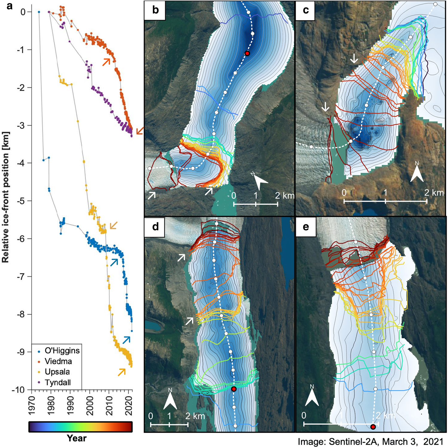
Figure 5. (a) Relative ice-front position change of the studied glaciers. Ice-front positions of (b) O'Higgins, (c) Viedma, (d) Upsala and (e) Tyndall glaciers. The colour of the ice front represents the date of the analysed image. The white arrows highlight the rapid retreat observed at O'Higgins, Viedma and Upsala glaciers. The white dashed line was used to interpolate the ice-front position to calculate the relative ice-front position change. The distance of the centreline is indicated by white and red circles every 1 and 10 km, respectively.
Figure 6 shows temporal variations in ice-front position, surface speed, surface elevation and surface slope between 2000 and 2022. As the ice-front retreated stepwise since 2017, ice flow speed accelerated synchronously (Fig. 6a), implying a substantial increase in the frontal ablation rate. The ice flow speed was 2.0 km a−1 in the beginning of 2016, which increased slightly until the end of 2016 by 0.3 km a−1 (Figs 6a and 13). In January 2017, as the ice front retreated, the ice flow sped up substantially to 3.8 km a−1 (Fig. 6a). Another ice front retreat was observed in January 2019, accompanied by ice flow acceleration up to 4.2 km a−1 (Figs. 6a and 13). In early 2022, it further increased from 3.5 km a−1 to 5.4 km a−1 (Fig. 6a). The mean elevation lowering rate was calculated between 28 and 32 km along the centreline (Fig. 6b). It showed 17.6 m a−1 between 2017 and 2022, which is 11 times greater than that observed between 2000 and 2015 (1.6 m a−1) (Fig. 6b). The surface slope steepened during the rapid retreat after 2016 (Figs 6b and 14a). Between 2017 and 2022, the slope increased up to 6.2°, which was about 4.4° between 2000 and 2015 (Fig. 6b). The water depth at the ice-front position along the centreline shows that the ice front stayed slightly deeper in the water since 2016 (Fig. 6c), but still touched the bank opposed to the ice flow (Figs 5b and 6d). During the rapid retreat in 2017, water depth increased by 20 m, and the ice front detached from the bank (Figs. 5b and 6d). The water depth at the centreline of the ice front decreased by about 20 m during late 2017 and 2018 (Fig. 6c) and then the ice front became relatively stable (Fig. 6a). Since January 2019, the water depth increased again by 20 m because of the rapid retreat. While the further retreat was observed in 2021, the lake topography is not covered by our measurements (Fig. 5b).

Figure 6. (a) Time-series of ice speed (black and blue dots) and ice front position (green dots) for Glaciar O'Higgins. The grey line indicates annually averaged surface ice speed, weighted for temporal separations. Figure 13 shows the variables between 2014 and 2018. (b) Ice surface elevation (red dots) and surface slope (purple square). The dot-dash line is the best-fit linear regression line for the elevation change based on three DEMs between 2018 and 2022. (c) Water depth at the calving front along the centreline (black dots) and terminus position change rate (green line). Because our bathymetry data has limited coverage near the ice front, there are data gaps in the water depth in recent years. (d) Ice-front positions and lake topographies. Ice-front positions analysed in 2005, 2014, 2017 and 2018 are indicated in each panel with a colour code. (e) Height above buoyancy was calculated from surface elevation and bathymetry map of the glacier with an average error of ±14 m. The timing of the calculation is indicated by a black dot line in panels (a)–(d). The orange line highlights where the height above buoyancy is zero. Green lines indicate the retreated ice-front position after the floating condition, which is also indicated by the red square in panel (a). The longitudinal profile of the ice surface elevation along the centreline is depicted in Fig. 14a.
Figures 6d and e show the ice-front position, bed topography and the calculated height above buoyancy by assuming hydrostatic equilibrium in January 2005, April 2014, March 2016 and April 2018. In January 2005 and April 2014 the low value of the height above buoyancy indicates that the middle of the ice front is very close to floating condition, suggesting that ice front is still grounded (Figs. 6e and 14a). However, it shows ~10 m below the flotation level on both sides of the ice front when the glacier slightly accelerated (Fig. 6a), while retreating rapidly in early 2017 (Figs. 6a, d and e). The ice-front position was located at a similar place in 2018. Although our bathymetry covers only a part of the DEM, it shows the ice front is ~20 m below the flotation level in April 2018 (Figs. 6e and 14a). This part retreated in early 2019 (Figs. 6a, d and e).
4.2.2 Glaciar Viedma
The rate of retreat for Glaciar Viedma has gradually increased (Figs. 5a and 7a). It was 33 m a−1 between 2000 and 2012 and increased to 200 m a−1 between 2012 and 2021, punctuated by relatively large retreats in April 2013 and February 2016 (Fig. 7a, highlighted by green squares). While ice speed did not show a substantial change before 2014, the surface ice speed (~0.6 km a−1) starts to gradually accelerate after 2015 and reached a peak speed of 1.3 km a−1 in 2019 (Fig. 7a). Then, it showed a slight decrease towards 2021 (1.1 km a−1) with clear seasonality (Fig. 7a). The surface elevation showed a larger lowering rate between 2012 and 2022 (12.4 m a−1) than between 2000 and 2012 (5.0 m a−1) while the surface slope increased from around 1.8° to around 2.4° between 2012 and 2018 (Fig. 7b). The retreat, acceleration, thinning and steepening is coincident with an ice-front retreat into the deep water (Fig. 7c). The water depth increased from 420 m to 510 m due to the retreat in April 2013. Until March 2016, the ice front was stable at that depth but retreated further into deeper water around 700 m, when the width of the ice front also showed the greatest value (Fig. 5c).

Figure 7. Similar plots as in Figure 6 for Glaciar Viedma. (d) Note that two years of ice-front positions are indicated.
The floating level was calculated by using the surface and bed topographies in February 2012, February 2013, December 2015 and October 2016 (Figs 7e and 14b). While the glacier height was above flotation level in February 2012, it was below flotation level at the middle part of the ice front in February 2013 (Fig. 7e), coincident with the ice front's retreat into deep water (Fig. 7c). One of the largest retreats was observed at the beginning of 2016. The height above buoyancy calculated in December 2015 shows that the north-eastern part of the ice front was 10 to 20 m below zero (Fig. 7e). In October 2016, the middle part of the ice front showed a negative height above buoyancy, after which the ice front retreated over the deepest part of the lake (Fig. 14b).
4.2.3 Glaciar Upsala
The rapid ice front retreat initiated in 2008 was accompanied by ice flow acceleration and thinning, which have been reported by previous studies (Sakakibara and others, Reference Sakakibara, Sugiyama, Sawagaki, Marinsek and Skvarca2013; Sakakibara and Sugiyama, Reference Sakakibara and Sugiyama2014). In addition to their findings, we found that the ice speed and slope have gradually increased since 2005 (Figs. 8a and b). The rapid retreat and acceleration were initiated in 2008 (Fig. 8), when the ice front detached from the bedrock bump at 8 km of the centreline (Figs. 2g and 8d). During the rapid retreat between 2008 and 2011, the surface slope also increases at a rate of 0.24° a−1 (Fig. 8b). The mean surface lowering rate calculated between 2008 and 2012 was 29.5 m a−1, which is close to three times larger than that calculated between 2000 and 2021 (11.8 m a−1).

Figure 8. Similar plots as in Fig. 6 for Glaciar Upsala. (e) Note that the bedrock bump was observed at 55 km along the centreline.
The calculated height above buoyancy using surface elevation and bed topography shows that the ice front was well below the flotation level before the rapid retreat event occurred (Figs. 8d, e and 14c). Intriguingly, in the case of Glaciar Upsala, the retreated ice front appears to follow the contour line where height above buoyancy becomes zero (Fig. 8e). In February 2005, half of the eastern ice front was about 10 m below the floating condition and retreated in April 2005 as indicated by the green line (Fig. 8e). In February 2008, the terminus over the bedrock bump was above the flotation level, but it was 10 to 20 m below the flotation level 1 to 2 km up-glacier from the ice front, which retreated by May 2009 (Fig. 8e). Another calculation of the height above buoyancy in January 2009 suggests that while the ice front is located over the bump, the glacier height is well below the flotation level, suggesting no buttressing from the bedrock bump (Figs. 8e and 14c). When the ice speed, thinning rate and surface slope showed their maximum between the end of 2009 and the beginning of 2010, most parts of the ice front up to 2 km up-glacier was 20 m below the flotation level (Figs. 8e and 14c). A satellite image from December 2009 indicates that the margins of the lower part of the glacier were highly fractured and a marginal rift propagated from the western margin (Fig. 15a). The glacier front had calved off by May 2010 and generated tabular icebergs (Fig. 15b).
4.2.4 Glaciar Tyndall
Glaciar Tyndall has retreated almost at a near constant rate between 2000 and 2021 (79.6 m a−1), but the retreat was characterized by large episodic tabular iceberg calving events (Fig. 5a and 9a), observed in 2001 and 2010 (Figs. 15c, d). During the mid-2000, the ice front of Glaciar Tyndall developed a formation of long, narrow tongues (Fig. 5e). Dense mapping of the ice-front position since 2016 indicates that the ice front continuously advances for one to two years followed by occasional retreat by calving in the summer (Fig. 9a). There is no clear interannual variability in surface ice speed and surface slope (Figs. 9a and b). The surface elevation was lowered by 153 m between 2000 and 2021 (Fig. 9b). Water depth was similar for the ice front between 2000 and 2010, while the ice front width narrowed by 200 m during the same period (Fig. 9c). Since 2010 the water depth gradually increased from 380 m to 420 m (Fig. 9c).

Figure 9. Similar plots as in Fig. 6 for Glaciar Tyndall. (d) Note that two years of ice-front positions are indicated.
Height above buoyancy calculations suggested that the ice front of Glaciar Tyndall was in near- or super-buoyant conditions in 2000, 2005 and 2010 (Figs. 9e and 14d), where we have DEM overlapped with the lakebed topography (Fig. 9d). A relatively large retreat was observed in 2001 and 2010, where most of the ice front was 10 m below floating condition, calculated in February 2000 and July 2011 (Fig. 9e).
5. Discussion
We measured the detailed lake topography near the ice fronts of O'Higgins, Viedma, Upsala and Tyndall glaciers (Fig. 2). The resulting bathymetries show close relation with glacier's retreat, acceleration and thinning (Figs 6–9). The bathymetric data can be utilized to improve the estimation of ice discharge from the selected glaciers (Minowa and others, Reference Minowa, Schaefer, Sugiyama, Sakakibara and Skvarca2021), as well as for calibration and validation of ice thickness inversion methods (e.g. Morlighem and others, Reference Morlighem2011; Fürst and others, Reference Fürst2017). In this study, we utilize the data to investigate observed glacier dynamics and discuss possible mechanisms of rapid changes in ice flow, glacier calving and ice-front position. We also discuss the difference between lake-terminating glaciers in Patagonia and calving glaciers in other regions of the world.
5.1 Importance of a super-buoyant ice front for the rapid glacier mass loss
Comparison of bedrock topography with ice-front position and ice speed shows that lake topography controls the rapid retreat observed at O'Higgins, Viedma and Upsala glaciers (Figs 6–9). We observed gradual ice speed acceleration at Glaciar O'Higgins in 2016 prior to its rapid retreat and acceleration (Figs 6 and 13). Noisier but similar gradual ice speed acceleration was observed at Glaciar Upsala since 2005 prior to its rapid retreat in 2008 (Fig. 8a) as reported by Sakakibara and others (Reference Sakakibara, Sugiyama, Sawagaki, Marinsek and Skvarca2013). At Glaciar Viedma, ice flow gradually increased for multiple years since 2012 (Fig. 7a). The calculation of flotation level suggests that the ice front was in a super-buoyant condition, and that also further upstream the glacier was near buoyant condition during the gradual flow acceleration of those glaciers (Figs. 6e, 7e, 8e and 14). These results suggest that the effective pressure decreased by losing overburden ice pressure and parts of the ice front decoupled from the bed, resulting in an increase of basal sliding near the ice front.
After the gradual ice flow acceleration, rapid glacier retreat and acceleration were observed coincident with ice front retreat from different pinning points: the opposed bank at Glaciar O'Higgins (Fig. 5b), the bedrock bump at Glaciar Upsala (Fig. 5d) and shallow and narrow topography at Glaciar Viedma (Fig. 5c). A comparison of the ice-front position and height above buoyancy shows that the ice-front retreated approximately along the contour line of the height above buoyancy equals zero (Figs. 6e–9e). This implies that a buoyancy force acts on the terminus, and can cause it to develop basal crevasses through a concentration of large basal tensile stresses and eventually triggers a large-scale and full-thickness iceberg calving event (e.g. Parizek and others, Reference Parizek2019; Trevers and others, Reference Trevers, Payne, Cornford and Moon2019). The rapid flow acceleration followed by ice front detachment from the pinning point suggests that a sudden change in the force balance due to a strong reduction in basal friction caused substantial ice flow acceleration (O'Neel and others, Reference O'Neel, Pfeffer, Krimmel and Meier2005; Howat and others, Reference Howat, Joughin and Scambos2007). On the other hand, a more gradual acceleration was observed in Glaciar Viedma, which has narrower lake bedrock topography than Glaciar O'Higgins and Glaciar Upsala (Figs. 2 and 4). Glaciar Tyndall did not show any flow acceleration even after the glacier retreated into deeper water (Figs. 9 and 14d). These differences might indicate that lateral shear stress makes an important contribution to the force balance near the front of Viedma and Tyndall glaciers due to narrower lake topography (Fig. 4). Viedma and Tyndall glaciers have lower flow speed than Upsala and O'Higgins glaciers, resulting in lower stresses to fracture ice. This idea seems to be plausible, as we observe less crevasses in satellite images and in the field in Viedma and Tyndall glaciers. Less fractured ice for those glaciers may have more resistance to the buoyancy force.
The substantial flow acceleration is accompanied by an increase in glacier calving and therefore ice front retreat in O'Higgins, Viedma and Upsala glaciers (Figs 6–8). Our results indicate that super-buoyant conditions play an important role in calving and retreat. The short-lived floating condition is supported by the tabular icebergs observed in front of Glaciar Upsala during the rapid retreat between 2008 and 2011 (Fig. 15b). Two tabular icebergs, with approximate dimensions of 600 × 500 m and 300 × 800 m, float in Brazo Upsala (Fig. 15b). Our height above buoyancy calculation indicated that these icebergs were generated from the region where more than 2 km of the ice front was in a floating condition (Figs. 8e and 14c). In addition to increased fracturing due to the acceleration of ice flow, the buoyancy force might generate a full-thickness crevasse from the base of the glacier (Parizek and others, Reference Parizek2019; Trevers and others, Reference Trevers, Payne, Cornford and Moon2019), resulting in tabular icebergs and rapid retreat (e.g. van der Veen, Reference van der Veen2002; Benn and others, Reference Benn, Warren and Mottram2007). Previous studies found that increased ice flow, high water pressure at the grounding line and buoyancy torque favour the development of basal crevasses (van der Veen, Reference van der Veen1998; Nick and others, Reference Nick, Van der Veen, Vieli and Benn2010). We did not observe any similar tabular icebergs in front of O'Higgins and Viedma glaciers and the height above buoyancy calculation suggests that the floating part is relatively limited when compa red with that observed in front of Glaciar Upsala (Figs. 6e and 7e). Whether an iceberg capsizes or not is determined by the aspect ratio of the iceberg's width and thickness (Burton and others, Reference Burton2012). The limited region of the floating portion suggests that even though there is full-thickness calving, the iceberg capsizes and breaks off into pieces. These type of floating conditions near a glacier front was suggested to exist at ocean-terminating glaciers (Howat and others, Reference Howat, Joughin, Tulaczyk and Gogineni2005, Reference Howat, Joughin and Scambos2007, Reference Howat, Joughin, Fahnestock, Smith and Scambos2008; Joughin and others, Reference Joughin2008).
In contrast, we observed a near flotation ice front for three available DEMs between 2000 and 2010 at Glaciar Tyndall without observing acceleration and rapid retreat (Fig. 9). At Glaciar Tyndall, we also observed tabular icebergs in 2005 and 2017 with dimensions similar to those observed in front of Glaciar Upsala (Figs. 15c and d). Compared with the other three glaciers, Glaciar Tyndall has a much lower flow speed (~500 m a−1) and flows into a shallower lake (300 to 400 m). We speculate that due to the lower flow speed of the glacier, it might have less fractured ice and that the buoyancy for this glacier might result in the formation of a floating tongue.
While our analyses suggest the importance of an ungrounded ice front in flow acceleration and large-scale calving at lake-terminating glaciers, our floating-level calculation is limited in time. Analysing floating conditions and ice flow more frequently will eventually improve our understanding of the cause of flow acceleration and iceberg calving. If the bedrock topography is known, these analyses can be accomplished by oblique photogrammetry (James and others, Reference James, Murray, Selmes, Scharrer and O'Leary2014; Murray and others, Reference Murray2015) or terrestrial radar interferometry (Parizek and others, Reference Parizek2019; Walter and others, Reference Walter, Lüthi and Vieli2020; Cook and others, Reference Cook, Christoffersen, Truffer, Chudley and Abellan2021). However, such field observations are usually conducted in the summer months. Capturing the whole process of the rapid retreat is still challenging and can take several years in the case of Patagonian glaciers.
5.2 Rapid retreat of Glaciar Upsala
Of the glaciers in this study, the ice front retreat and acceleration were the strongest at Glaciar Upsala, resulting in the formation of marginal rifts and calving of tabular icebergs (Figs. 6–9 and 15). Longitudinal and shear strain rates were calculated based on the satellite-derived velocities before and after the event at Glaciar Upsala (Fig. 10). The strain rate tensor is calculated by spatially differentiating the velocity field in initially Universal Transverse Mercator coordinates system and rotated with ice flow direction (e.g. Stearns and others, Reference Stearns2015). Two velocity fields were used to calculate strain rates between 28th September and 14th October in 2001, and between 14th and 30th August in 2008. In both cases, the velocity was determined over the entire region near the ice front (Figs. 10a and d). Uncertainties in the calculated strain rates originating from the errors in the velocity fields were 0.5 a−1 for 2001 and 0.8 a−1 for 2008 on average.

Figure 10. (a) Surface ice speed, (b) longitudinal strain rate and (c) shear strain rate calculated between 28th September and 14th October 2001 in Glaciar Upsala. Grey arrows show flow direction. (d)–(f) Calculated between 14th and 30th August 2008, when the glacier showed acceleration and rapid ice-front retreat (Fig. 8). (d) The orange line indicates the place where the height above buoyancy becomes zero calculated with ASTER DEM of January 2009 (Fig. 8e). (g) Changes in surface ice speed, (h) longitudinal strain rate and (i) shear strain rate were calculated by subtracting the 2008 data from the 2001 data. (h) and (i) The marginal rift observed on the satellite image of December 2009 is indicated by a red line. The centreline of the glacier is shown by white circles, dotted every 1 km. At 55 km of the centreline, a bump was observed in the lake topography (Fig. 2g).
The flow speed increased all over the lower part of the glacier terminus in 2008 in comparison to 2001 (Figs. 10a, d and g), and was particularly enhanced over the western part of the terminus up to 1 km a−1 (Fig. 10g). The strongly accelerated part appears to be coincident with the place where the glacier floated as inferred from the height above buoyancy calculation (orange line in Figs. 10d and g). Most notably, the shear strain rate over the western margin in the lower part of the glacier varied between 2001 and 2008 (Figs. 10c, f and i). The substantial flow acceleration due to the decoupling of ice from the base caused contrasting flow speed differences between the margin and central part of the ice flow, which enhanced the shear strain rate in that region. Interestingly, the marginal rift observed on December 2009 was developed over the western margin, where high ice fracture is expected due to the high shear strain rates (Figs. 10i and 15a). Similar rift development and propagation into fast flow are often observed on ice shelves in Antarctica (e.g. Alley and others, Reference Alley, Scambos, Alley and Holschuh2019; Benn, Reference Benn2022) and Greenland (e.g. Falkner and others, Reference Falkner2011), due to strong flow speed contrast between marginal and central parts of the ice shelf. To our knowledge, this process has never been reported for lake-terminating glaciers. The strong flow acceleration due to the transient floating tongue and overdeepening may be the cause of this rare calving event observed at Glaciar Upsala (Fig. 15b).
5.3 Comparison of Patagonian lake-terminating glaciers with calving glaciers in other regions
Because the ice flow, calving and changes in ice-front position are closely related to water depth near the terminus of calving glaciers, we compared width-averaged water depth and frontal ablation rate among the calving glaciers in Patagonia (Warren and others, Reference Warren1995a, Reference Warren, Greene and Glasser1995b; Warren and Aniya, Reference Warren and Aniya1999; Rignot and others, Reference Rignot, Forster and Isacks1996; Rivera and others, Reference Rivera, Lange, Aravena and Casassa1997; Rott and others, Reference Rott, Stuefer, Siegel, Skvarca and Eckstaller1998), Alaska (Brown and others, Reference Brown1982; Meier and others, Reference Meier, Rasmussen and Miller1985; Funk and Röthlisberger, Reference Funk and Röthlisberger1989; Pelto and Warren, Reference Pelto and Warren1991; Motyka and others, Reference Motyka, Hunter, Echelmeyer and Connor2003), Greenland (Funk and Röthlisberger, Reference Funk and Röthlisberger1989; Pelto and others, Reference Pelto, Hughes and Brecher1989; Pelto and Warren, Reference Pelto and Warren1991), New Zealand (Hochstein and others, Reference Hochstein1995; Warren and Kirkbride, Reference Warren and Kirkbride2003), Alps (Funk and Röthlisberger, Reference Funk and Röthlisberger1989), Iceland (Björnsson and others, Reference Björnsson, Pálsson and Guðmundsson2001), Norway (Laumann and Wold, Reference Laumann and Wold1992) and Svalbard (Pelto and Warren, Reference Pelto and Warren1991) (Fig. 11 and supplementary dataset). Width-averaged frontal ablation rate a (sum of iceberg calving and subaqueous ice cliff melting) was estimated by subtracting the width-averaged ice speed near the terminus (u m) with the change of ice-front position (dL/dt): a = u m− dL/dt. We used annual mean ice speed and mean change of ice-front position in 2001 to calculate the frontal ablation rate because of the abundant availability of ice-front position, surface speed and water depth data to calculate annual mean frontal ablation rate (Supplementary dataset). In addition to this, both the ice speed and the change of ice-front position vary strongly during the dynamic glacier retreat (Figs. 6–9). Thus, the frontal ablation rate was calculated in 2001 to avoid such influences when comparing with other glaciers. Width-averaged water depth was obtained from cross-sectional profiles based on the observed water depth, set close to the ice front in 2001.

Figure 11. (a) Comparison between width-averaged water depth and frontal ablation rate for lake-terminating glaciers. Colour of the markers indicates the region of the lake-terminating glaciers: PT–Patagonia, AK–Alaska, GL–Greenland, NZ–New Zealand, AP–Alps, IL–Iceland and NW–Norway. Inset shows an enlarged plot of water depth against frontal ablation rate for shallow water glaciers less than 50 m deep. (b) A similar plot for lake-terminating glaciers in Patagonia (PT) is indicated by circles and ocean-terminating glaciers in Alaska (AK), Greenland (GL) and Svalbard (SB) are indicated by squares. Dataset sources are summarized in the supplementary dataset.
Compared to lake-terminating glaciers in other regions, the Patagonian glaciers terminate in much deeper lakes ranging between 100 and 500 m and experience higher frontal ablation rates (Fig. 11a). The deep lakes in Patagonia appear to be developed by a high glacial erosion rate due to a warm climate, abounded subglacial discharge and high basal sliding (Koppes and others, Reference Koppes2015). The great depth near the glacier terminus causes greater flow in the Patagonian glaciers compared to the calving glaciers in other regions, resulting in larger frontal ablation. It may also explain the greater retreat and thinning rates at O'Higgins, Upsala and Viedma glaciers compared to lake-terminating glaciers in Alaska (Boyce and others, Reference Boyce, Motyka and Truffer2007; Trüssel and others, Reference Trüssel, Motyka, Truffer and Larsen2013), the Alps (Tsutaki and others, Reference Tsutaki, Sugiyama, Nishimura and Funk2013) and Himalaya (Sato and others, Reference Sato2022). The accelerated flow, thinning rate and retreat rate reached 1–6 km a−1, 10–50 m a−1 and 0.4–0.8 km a−1, respectively, for those three glaciers in Patagonia, while these numbers were one to two orders of magnitude smaller in the lake-terminating glaciers in the other regions (Boyce and others, Reference Boyce, Motyka and Truffer2007; Tsutaki and others, Reference Tsutaki, Sugiyama, Nishimura and Funk2013; Trüssel and others, Reference Trüssel, Motyka, Truffer and Larsen2013; Sato and others, Reference Sato2022). We expect there are several factors causing this difference: Patagonian lake-terminating glaciers are relatively thick, experience high surface slopes and flow into wide and deep lakes, resulting in higher driving stress and ice speed. In such conditions, the increase in the ice speed near the terminus of the glaciers in Patagonia can result in a greater magnitude of the dynamic thinning than the calving glaciers in the other regions.
Lake-terminating glaciers are usually expected to experience lower frontal ablation rates compared to ocean-terminating glaciers, which is also supported by our study (Fig. 11b). In particular, a clear contrast can be found between the lake-terminating glaciers in Patagonia and the ocean-terminating glaciers in Alaska, both located in similar maritime climate settings. The frontal ablation estimated for Glaciar San Rafael in Patagonia, which flows into a brackish water, is in line with those reported for ocean-terminating glaciers in Alaska (Fig. 11b). Lake-terminating glaciers in Patagonia have contrasting processes occurring at their front compared to ocean-terminating glaciers due to the difference of water density in front of the glaciers (Sugiyama and others, Reference Sugiyama2016; Truffer and Motyka, Reference Truffer and Motyka2016). The fresh and turbid subglacial water discharge into the fjords generates an upwelling plume, which effectively entrains the warm deep water to melt the ice under the water (e.g. Motyka and others, Reference Motyka, Hunter, Echelmeyer and Connor2003, Reference Motyka, Dryer, Amundson, Truffer and Fahnestock2013). In contrast, the subglacial discharge normally stays deep in freshwater lakes and limits subaqueous melting (Sugiyama and others, Reference Sugiyama2016, Reference Sugiyama2021; Minowa and others, Reference Minowa, Sugiyama, Sakakibara and Skvarca2017). Active submarine melting may destabilize the subaerial part of the calving front and enhance glacier calving for the ocean-terminating glaciers. The limited amount of subaqueous melting in the lakes favours keel development, which may in the end cause buoyancy-driven large-scale calving (Purdie and others, Reference Purdie, Bealing, Tidey, Gomez and Harrison2016; Sugiyama and others, Reference Sugiyama, Minowa and Schaefer2019). Additionally, the water density difference causes a higher buoyancy force for ocean-terminating glaciers than for lake-terminating glaciers. van der Veen (Reference van der Veen2002) pointed out that effective pressure more substantially decreases when the ice front is close to flotation for an ocean-terminating glacier than for a lake-terminating glacier. These differences may result in greater ice front retreat, acceleration and thinning in ocean-terminating glaciers in Alaska (e.g. O'Neel and others, Reference O'Neel, Pfeffer, Krimmel and Meier2005; Pfeffer, Reference Pfeffer2007) and Greenland (e.g. Howat and others, Reference Howat, Joughin, Tulaczyk and Gogineni2005, Reference Howat, Joughin and Scambos2007, Reference Howat, Joughin, Fahnestock, Smith and Scambos2008; Joughin and others, Reference Joughin2008; Catania and others, Reference Catania2018).
Many calving glaciers have shown retreat and thinning over the last several decades in Patagonian icefields (e.g. Aniya and others, Reference Aniya, Sato, Naruse, Skvarca and Casassa1997; Rignot and others, Reference Rignot, Rivera and Casassa2003; Sakakibara and Sugiyama, Reference Sakakibara and Sugiyama2014; Minowa and others, Reference Minowa, Schaefer, Sugiyama, Sakakibara and Skvarca2021). The dynamic retreat which accompanied flow acceleration was observed for several glaciers, which dominated the mass loss in the entire region (Minowa and others, Reference Minowa, Schaefer, Sugiyama, Sakakibara and Skvarca2021). Yet, bedrock topography is coarse, and coverage is especially limited in the lower ablation area, which is the most important place to interpret the fluctuation of outlet glaciers in Patagonia (Gourlet and others, Reference Gourlet, Rignot, Rivera and Casassa2016; Millan and others, Reference Millan2019). Since these dynamic retreats are highly sensitive to bedrock topography, further observations are strongly recommended to understand the fate of glaciers in Patagonia. Archiving such high-resolution topography datasets is still very challenging for gravity surveys due to the large spatial footprint. For ice radars, the measurements are challenging, particularly in lower parts of the glacier due to the influence of deep valleys, crevasses and the abundance of water in temperate ice (Zamora and others, Reference Zamora2009; Gourlet and others, Reference Gourlet, Rignot, Rivera and Casassa2016; Millan and others, Reference Millan2019). Modelling studies on the future evolution of calving glaciers using these coarse topography maps should be aware of the uncertainties in bed topography.
6. Conclusions
We measured the lake topography near the terminus of O'Higgins, Viedma, Upsala and Tyndall glaciers in the southern Patagonian icefield, which terminate in freshwater lakes. Ice-front position, ice speed, surface elevation, and surface slope of these glaciers were analysed based on multiple optical remote sensing datasets over the last several decades and compared with lake topography. O'Higgins, Viedma and Upsala glaciers showed high sensitivity to changes in their near terminus geometry, while Glaciar Tyndall did not. We hypothesized that the less sensitive behaviour of Glaciar Tyndall is due to the shallower and narrower lake than other lakes resulted in less ice flow and less importance of the buoyancy force near the ice front.
A rapid retreat was observed at O'Higgins and Viedma glaciers from 2016 onwards, and at Glaciar Upsala between 2008 and 2011. Floating level calculation suggests that the overdeepening basins and long-term thinning has caused a transiently super-buoyant condition near the terminus. Ice flow gradually increased when the floating condition or super-buoyant condition was reached near the ice front. Basal sliding is probably enhanced due to the reduced effective pressure or loss of basal drag due to the decoupling of the ice front from the ground. Large ice-front retreat occurred over the regions where super-buoyant conditions were observed. Once the ice front detached from the pinning point due to buoyancy-driven iceberg calving, ice flow accelerates by losing resistance force from the bedrock, and the glacier thins substantially due to the dynamic thinning. Further studies are desirable that consider the influence of meteorological and/or limnological conditions on the surface lowering to understand the trigger of the sequence of the rapid glacier mass loss.
The lake-terminating glaciers in Patagonia flow into deeper lakes than lake-terminating glaciers in other regions, resulting in larger ice flow and frontal ablation and greater potential for dynamic ice mass loss. Yet, it is not clear whether the observed rapid mass loss in Patagonian icefields will continue, as there is a lack of a reliable high-resolution bedrock topography data. Further observations of bed geometry with ice radar and gravity measurements will certainly help to understand the fate of Patagonian glaciers. Numerical projections should consider the uncertainty associated with the very high sensitivity of glacier dynamics to bedrock geometry near the ice front.
Supplementary material
The supplementary material for this article can be found at https://doi.org/10.1017/jog.2023.42.
Data availability
The water depth data presented in this paper will be publicly available at http://doi.org/10.5281/zenodo.7112456. The satellite dataset used in the study was acquired from the following portal sites (last accessed April 1, 2022): https://earthexplorer.usgs.gov/ (Landsat 8), https://scihub.copernicus.eu/ (Sentinel-2A, 2B), https://gbank.gsj.jp/madas/ (ASTER-VA) and https://www2.jpl.nasa.gov/srtm/ (SRTM). Calculated ice-front positions, surface ice speeds and DEMs are available upon reasonable request from the authors.
Acknowledgements
Bathymetry measurements were supported by various agencies, companies and individuals: Intendencia Parque Nacional Los Glaciares, Jorge Lenz Seccional Lago Viedma, Prefectura Naval Lago Argentino and Empresa Hielo y Aventura in Lago Argentino, Argentina. CONAF (Corporacion Nacional Forestal) in Lago O'Higgins, and Rodrigo Traub and Daniel Rutllant in Lago Geike, Chile. We thank Daiki Sakakibara for sharing his ice speed dataset and Shin Sugiyama for loaning the depth sounder. The manuscript was handled by the Scientific Editor Matthew Siegfried, and was improved by comments and suggestions from two anonymous reviewers. English text was corrected by Ariah Kidder. MM was supported by JSPS Overseas Research Fellowship (#20180152), Grant-in-Aid for JSPS Fellow (JP20J00526), and JSPS KAKENHI Grant (JP22K14093). FONDECYT regular grant (#1180785) provided financial support for field data collection.
Authors’ contribution
MM conceived the study with support from MS and PS at each stage of the study. MS and PS contributed to the bathymetry survey. All authors discussed the results and commented jointly on the manuscript.
Appendix

Figure 12. An overview of the available dataset for (a) O'Higgins, (b) Viedma, (c) Upsala and (d) Tyndall glaciers. The timing of the bathymetry survey is indicated by the blue circle. The horizontal green and red bars indicate the available period of optical Sentinel 2 and Landsat 8 images used for analysing the ice-front position and surface ice speed in this study. We combined data analysed by using Landsat 5, 7 and 8 images in previous studies (Sakakibara and Sugiyama, Reference Sakakibara and Sugiyama2014; Minowa and others, Reference Minowa, Schaefer, Sugiyama, Sakakibara and Skvarca2021) as indicated by a grey horizontal bar. Black squares, orange triangles and purple triangles indicate available DEMs obtained by SRTM mission, ASTER satellite and ALOS satellite, respectively.

Figure 13. Surface ice speed and ice front position observed at Glaciar O'Higgins between 2014 and 2018. Grey line indicates smoothed surface ice speed using a Gaussian smoothing routine with a time window of 90 days.

Figure 14. Longitudinal profiles of the ice surface elevations and slopes along the centreline at every 50 m in the horizontal interval for (a) Glaciar O'Higgins, (b) Glaciar Viedma, (c) Glaciar Upsala and (d) Glaciar Tyndall. The colour of the lines indicates the date. Red, blue and brown lines represent the flotation height, lake level and bed elevation, respectively. The dot-dashed line is the glacier base assuming hydrostatic equilibrium. The surface slope was calculated after applying the moving average on the surface elevation with a span of 2 km.

Figure 15. Tabular icebergs observed at (a) and (b) Glaciar Upsala, and (c) and (d) at Glaciar Tyndall. Note that the scale of the satellite images is different depending on the glacier.


 Open access