


1. Introduction
Nucleate-boiling heat transfer is one of the most efficient modes of heat transfer under high heat-flux conditions, and it is used in many engineering applications, such as refrigeration, cooling systems, boilers and heat exchangers. Although there are a multitude of applications, identification of the principal mechanisms driving the heat-transfer process still remains an area of active research. One of the main uncertainties is the role of microlayer formation and evaporation in the overall dynamics, as well as its relationship to the occurrence of departure from nucleate boiling.
The microlayer, presumed to be located at the base of a growing bubble on a horizontal, hot surface, as shown schematically in figure 1, is a layer of liquid with thickness less than a few micrometres, and has been observed to form beneath vapour bubbles during nucleate boiling under certain conditions (Kim Reference Kim2009). The microlayer extends from the liquid bulk up to the so-called contact-line region (also referred to as the microregion, and labelled as such in the figure), where vapour and liquid meet on the hot surface; this is followed by a dry patch (Kim Reference Kim2009). The dry patch is sometimes assumed to be covered by an adsorbed film of molecular thickness, presenting no resistance to heat transfer (Schweikert, Sielaff & Stephan Reference Schweikert, Sielaff and Stephan2019). Recent numerical evidence (Hänsch & Walker Reference Hänsch and Walker2016; Guion et al. Reference Guion, Afkhami, Zaleski and Buongiorno2018; Urbano et al. Reference Urbano, Tanguy, Huber and Colin2018) suggests that the microlayer profile is not of monotonic shape, but rather features a thickened region, or ‘hump’, immediately adjacent to the microregion (see inset to figure 1). Such a profile, i.e. a thin liquid film on a solid wall terminated by a hump, can also be observed during adiabatic dewetting of partially wetting fluids (Snoeijer et al. Reference Snoeijer, Andreotti, Delon and Fermigier2007; Delon et al. Reference Delon, Fermigier, Snoeijer and Andreotti2008).

Figure 1. Schematic visualisation of the microlayer located at the base if a growing bubble during nucleate boiling. Inset (top right) illustrates the termination of the microlayer by a ‘hump’.
After its formation, the microlayer appears to begin to evaporate rapidly, contributing significantly to the overall heat-transfer mechanism (Yabuki & Nakabeppu Reference Yabuki and Nakabeppu2017). While the reported contribution of microlayer evaporation to the overall bubble growth is still disputed in the literature (Kim Reference Kim2009), more recent measurements indicate contributions of 15 %–50 % to the growth, depending on the fluid chosen and the exact experimental conditions (Yabuki & Nakabeppu Reference Yabuki and Nakabeppu2014; Utaka et al. Reference Utaka, Hu, Chen and Morokuma2018), with locally measured heat-flux values in the microlayer reaching  $1\ \textrm {MW}\ \textrm {m}^{-2}$ (Yabuki & Nakabeppu Reference Yabuki and Nakabeppu2014). This suggests that the microlayer dynamics is of considerable importance in the nucleate-boiling process.
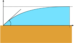
The actual presence of a microlayer during nucleate boiling is not always guaranteed: for example, if the bubble growth is sufficiently slow, a microlayer is not always observed, and then the overall bubble shape remains essentially spherical (Son, Dhir & Ramanujapu Reference Son, Dhir and Ramanujapu1999; Fischer et al. Reference Fischer, Herbert, Slomski, Stephan and Oechsner2014; Huber et al. Reference Huber, Tanguy, Sagan and Colin2017; Urbano et al. Reference Urbano, Tanguy, Huber and Colin2018). In this so-called contact-line regime, the liquid bulk surrounding the bubble is sharply terminated by the presence of a dry patch, as shown in figure 2. Note that the absence of a microlayer significantly reduces the overall heat transfer.

Figure 2. Schematic visualisation of the contact-line nucleate-boiling regime.
As the transition between the contact-line regime of boiling and boiling in the presence of a microlayer (microlayer evaporation regime) results in qualitative changes in the overall dynamics, identifying the conditions under which microlayer formation takes place is crucial for a full understanding of the nucleate-boiling heat-transfer process. Conceptually, growth of a bubble on a solid surface during nucleate boiling represents an example of dewetting in the presence of phase change. Problems involving adiabatic dewetting are well known to feature qualitative regime transitions associated with a certain critical velocity: e.g. droplets undergo a shape transition if they are sliding ‘too quickly’ along a surface (Le Grand, Daerr & Limat Reference Le Grand, Daerr and Limat2005), and a liquid film, known as the Landau–Levich film (Levich & Landau Reference Levich and Landau1942), is known to adhere to a plate if it is withdrawn from a liquid bath sufficiently fast.
The hypothesis that the microlayer formation mechanism could be understood in terms of a dewetting transition in the presence of phase change has been discussed frequently in the past (more recently by Afkhami et al. Reference Afkhami, Buongiorno, Guion, Popinet, Saade, Scardovelli and Zaleski2018; Guion et al. Reference Guion, Afkhami, Zaleski and Buongiorno2018). Also, Schweikert et al. (Reference Schweikert, Sielaff and Stephan2019) performed the plate-withdrawal experiment for a volatile liquid in order to understand the transition between the contact-line and microlayer evaporation regimes: they observed the occurrence of a wetting transition qualitatively similar to that of the adiabatic case (i.e. the Landau–Levich transition). Furthermore, Urbano et al. (Reference Urbano, Tanguy, Huber and Colin2018) simulated numerically microlayer formation during nucleate boiling using direct numerical simulation (DNS), and suggested that a microlayer would be formed if the radial bubble expansion velocity exceeded a certain critical value, which the authors estimated from a fit to the DNS data they obtained.
In view of the available evidence, we support the hypothesis of microlayer formation based on dewetting. Furthermore, we believe that it is possible to quantify the threshold criterion between the contact-line evaporation regime and the microlayer evaporation regime. Consequently, in this work, we propose a correlation for this transition based on the Cox–Voinov law for volatile liquids in § 2, which we then validate in § 3 using the experimental data of Schweikert et al. (Reference Schweikert, Sielaff and Stephan2019). In § 4, we extend the application of the criterion to nucleate boiling and compare results to the DNS data of Urbano et al. (Reference Urbano, Tanguy, Huber and Colin2018). We discuss also, in general terms, the relative benefits and limitations of DNS investigations of microlayer dynamics. Furthermore, we speculate on the initial microlayer thickness following its formation. Finally, overall conclusions are drawn in § 5. Additionally, appendix A details results of our own simulations of microlayer formation that we have performed to support the arguments developed in the paper.
2. Criterion formulation
In the context of dynamic, adiabatic wetting phenomena, analytic solutions of quasi-static, contact-line motion have resulted in constitutive laws being proposed connecting an apparent contact angle  $\theta _{app}$ (the macroscopically observed interfacial slope) with the microscopic contact angle $\theta _0$ (described below) and the capillary number $Ca$ (Snoeijer et al. Reference Snoeijer, Andreotti, Delon and Fermigier2007; Bonn et al. Reference Bonn, Eggers, Indekeu, Meunier and Rolley2009), viz
 \begin{equation} \theta_{app} = f(Ca,\theta_0). \end{equation}
The capillary number is given as
 \begin{equation} Ca = \frac{\mu_l U_{CL}}{\sigma}, \end{equation}
with  $U_{CL}$ being the contact-line velocity along the surface ( $\textrm {m}\ \textrm {s}^{-1}$), $\sigma$ the surface tension ( $\textrm {N}\ \textrm {m}^{-1}$) and $\mu _l$ the liquid dynamic viscosity ( $\textrm {Pa}\ \textrm {s}$). The microscopic contact angle is conventionally assumed to be constant (i.e. any hysteresis effects are neglected), and to result from a force balance at the triple line (Snoeijer et al. Reference Snoeijer, Andreotti, Delon and Fermigier2007). A prominent example of (2.1) is the Cox–Voinov law, written with the dewetting sign convection (Voinov Reference Voinov1976; Cox Reference Cox1986) as
 \begin{equation} \theta_0^3-\theta_{app}^3 = \frac{\textit{Ca}}{A}. \end{equation}
This law has been shown to represent measured experimental data in a variety of configurations: for example in droplet sliding (Le Grand et al. Reference Le Grand, Daerr and Limat2005), spreading (Kant et al. Reference Kant, Hazel, Dowling, Thompson and Juel2017) and spreading with solidification (de Ruiter et al. Reference de Ruiter, Colinet, Brunet, Snoeijer and Gelderblom2017). The constant  $A$ is unknown a priori and is usually determined by a fit to experimental data. Equation (2.3) was also found to hold in the presence of liquid-to-vapour phase change by Janeček & Nikolayev (Reference Janeček and Nikolayev2013) from a numerical solution of the lubrication equations, coupled with steady-state one-dimensional heat conduction. However, in this context, the equation takes the form (Fourgeaud et al. Reference Fourgeaud, Ercolani, Duplat, Gully and Nikolayev2016)
 \begin{equation} \theta_{mr}^3(\Delta T,\textit{Ca}=0)-\theta_{app}^3 = \frac{\textit{Ca}}{A}, \end{equation}
where  $\theta _{mr}(\Delta T,{Ca}=0)$ is the static contact angle for the volatile liquid under non-isothermal conditions, which takes into account the effect of phase change in the microregion on the interfacial slope. We will denote this quantity by the symbol $\theta _{mr}$ and, for brevity, refer to it as the non-adiabatic contact angle. The actual value of $\theta _{mr}$ can be non-zero, even for fully wetting liquids (Raj et al. Reference Raj, Kunkelmann, Stephan, Plawsky and Kim2012; Fourgeaud et al. Reference Fourgeaud, Ercolani, Duplat, Gully and Nikolayev2016; Schweikert et al. Reference Schweikert, Sielaff and Stephan2019). Note that (2.4) essentially states that the effect of phase change ( $\Delta T$) and contact-line motion (Ca) on the apparent contact angle can be decoupled (Janeček & Nikolayev Reference Janeček and Nikolayev2013; Fourgeaud et al. Reference Fourgeaud, Ercolani, Duplat, Gully and Nikolayev2016).
A wetting transition as  $\theta _{app}\rightarrow 0$ has already been conjectured by Derjaguin & Levi (Reference Derjaguin and Levi1964), analytically derived by Eggers (Reference Eggers2005) and numerically confirmed by Snoeijer et al. (Reference Snoeijer, Andreotti, Delon and Fermigier2007). Note that, in this last paper, it was shown that, at the transition point, the solutions undergo a series of saddle-node bifurcations, featuring a non-monotonically shaped film, and asymptotically tending to an infinitely long flat film behind the contact line. Under the condition $\theta _{app}=0$, (2.4) immediately gives, at the transition
 \begin{equation} \theta_{mr}^3 = \frac{{Ca}}{A}. \end{equation}
Rearranging, and using (2.2), we obtain a corresponding relation for the critical contact-line velocity as
 \begin{equation} U_{CL,{crit}}=\frac{\sigma}{\mu_l}A\theta_{mr}^3, \end{equation}
and we identify the condition  $U_{CL}\geqslant U_{CL,{crit}}$ with liquid-film (i.e. microlayer) formation due to dewetting transition.
For the value of  $A$, results of sliding droplet experiments suggest a value of $A\approx 4.5\times 10^{-3}$ for water (Podgorski, Flesselles & Limat Reference Podgorski, Flesselles and Limat2001; Winkels et al. Reference Winkels, Peters, Evangelista, Riepen, Daerr, Limat and Snoeijer2011). This value is considered to be anomalously low, and possibly reflective of the occurrence of non-hydrodynamic dissipative mechanisms near the contact line (de Ruiter et al. Reference de Ruiter, Colinet, Brunet, Snoeijer and Gelderblom2017). For sliding droplets, constituted by a silicone oil–water mixture, a value of $A\approx 10^{-2}$ has been proposed (Podgorski et al. Reference Podgorski, Flesselles and Limat2001; Le Grand et al. Reference Le Grand, Daerr and Limat2005; Winkels et al. Reference Winkels, Peters, Evangelista, Riepen, Daerr, Limat and Snoeijer2011), essentially independently of the degree of oil–water mixing. Generally, the choice of $A$ remains a source of uncertainty in (2.6), as it is a parameter dependent on properties of the test fluid, surface characteristics, solid–fluid interactions as well as on the particular geometry of the configuration. At the same time, theoretical predictions from the original Cox–Voinov law give (Bonn et al. Reference Bonn, Eggers, Indekeu, Meunier and Rolley2009)
 \begin{equation} A =\frac{1}{9\ln (S)}= \frac{1}{9\ln\left(l/a\right)}, \end{equation}
where  $S$ is a ratio of two scales: $a$ is a representative nanoscopic length scale. Under adiabatic conditions, it can be taken to be the typical molecule size, of the order of 0.1–1 nm (Podgorski et al. Reference Podgorski, Flesselles and Limat2001; Le Grand et al. Reference Le Grand, Daerr and Limat2005; Winkels et al. Reference Winkels, Peters, Evangelista, Riepen, Daerr, Limat and Snoeijer2011), or the slip length, a typical value for very smooth surfaces being 10 nm (Janeček & Nikolayev Reference Janeček and Nikolayev2013). In the context of microlayer formation, $a$ would be a typical scale of the microregion, of the order of 10–100 nm (Janeček Reference Janeček2012; Janeček & Nikolayev Reference Janeček and Nikolayev2013; Fourgeaud et al. Reference Fourgeaud, Ercolani, Duplat, Gully and Nikolayev2016), while $l$ represents a macroscopic dimension, dependent on the problem in question. The described configuration is summarised schematically in figure 3.

Figure 3. A visualisation of the film profile with a receding contact line. A dewetting transition occurs as the interfacial slope  $\theta _{app}\rightarrow 0$ at $x=l$, since $U_{CL}\geqslant U_{CL,crit}$. The inset (left) shows schematically the effect of phase change on the interfacial slope in the microregion. Length scales $l$ and $a$ from (2.7) are indicated.
3. Application of the criterion to experimental data on plate dewetting
With their experiments, Schweikert et al. (Reference Schweikert, Sielaff and Stephan2019) were able to produce a regime map of microlayer formation for the fluorocarbon FC-72 based on the values of the wall superheat  $\Delta T$ (up to 5 K) and a critical plate withdrawal velocity of up to $45\ \textrm {mm}\ \textrm {s}^{-1}$ (figure 9 in their paper). We have deduced the transition criterion directly from this figure to be (the plate-withdrawal velocity corresponding to the contact-line velocity)
 \begin{equation} U_{CL,{crit}}^{Schweikert}\ [\textrm{m}\ \textrm{s}^{{-}1}] = 3.12\times10^{{-}3} \Delta T^{1.44}. \end{equation}
By equating the plate-withdrawal velocity with the contact-line velocity, we have assumed that the principal effect of superheat in this experiment was to change the non-adiabatic contact angle, presuming the impact of phase change on the contact-line velocity to be minor, as indicated by Fourgeaud et al. (Reference Fourgeaud, Ercolani, Duplat, Gully and Nikolayev2016). Therefore, to apply our criterion to these data, we converted the applied superheats ( $\Delta T$) into $\theta _{mr}$ values. Although this could be done numerically with the help of a microregion model, such models do not generally predict the $\theta _{mr}=f(\Delta T)$ relationship accurately, as can be seen from the attempts by Raj et al. (Reference Raj, Kunkelmann, Stephan, Plawsky and Kim2012) and Janeček & Nikolayev (Reference Janeček and Nikolayev2013), especially for values of the superheat corresponding to the experimental conditions considered here. At the same time, FC-72 is known to be a non-polar liquid, fully wetting on the majority of surfaces (Reed & Mudawar Reference Reed and Mudawar1997; Raj et al. Reference Raj, Kunkelmann, Stephan, Plawsky and Kim2012; Schweikert et al. Reference Schweikert, Sielaff and Stephan2019), and thus $\theta _{mr}$ should be essentially independent of the surface material in question. Indeed, even if a microregion model had been used, the surface would be characterised only by the Hamaker constant (Israelachvili Reference Israelachvili2011; Raj et al. Reference Raj, Kunkelmann, Stephan, Plawsky and Kim2012), and the overall microregion model results would then be ‘very insensitive even to large variations of more than one order of magnitude’ of this constant (Raj et al. Reference Raj, Kunkelmann, Stephan, Plawsky and Kim2012), erasing any differences between the materials comprising these surfaces.
For this reason, we consider the experimental, non-adiabatic contact angle values for FC-72 originally measured for copper by Raj et al. (Reference Raj, Kunkelmann, Stephan, Plawsky and Kim2012) to be also applicable to the experimental conditions of Schweikert et al. (Reference Schweikert, Sielaff and Stephan2019), in spite of the difference in surface material (i.e. copper vs chromium, both found to be essentially perfectly wetted by FC-72 under adiabatic conditions by the respective authors). By using uncertainty-weighted, least-squares regression, together with a fit equation of the form
 \begin{equation} \theta_{mr} = C_0 \Delta T^{C_1}, \end{equation}
we recover the relation (see figure 4):
 \begin{equation} \theta_{mr,fit} \ [^{{\circ}}] = 9.37 \Delta T^{0.54}. \end{equation}
Evidently, much better agreement with experimental data has been achieved with our relation than with the microregion model-based solution given by Raj et al. (Reference Raj, Kunkelmann, Stephan, Plawsky and Kim2012), namely
 \begin{equation} \theta_{mr}^{\textit{Raj}}\ [^{{\circ}}] = 17.4 \Delta T^{0.323}, \end{equation}
especially in the interval of interest here,  $\Delta T\leqslant 5\ \textrm {K}$. In order to incorporate the effect of experimental uncertainties into our model, we also complement the best-estimate fit with two bounding predictions, obtained by performing unweighted least-squares regression on the data (i) reduced by one standard deviation ( $\theta ^{low}_{{mr}}$) and (ii) increased by one standard deviation ( $\theta ^{high}_{{mr}}$). The resulting fitted relations
 \begin{gather} \theta^{low}_{mr,fit} \ [^{{\circ}}] = 6.54 \Delta T^{0.65}, \end{gather}
 \begin{gather}\theta^{high}_{mr,fit} \ [^{{\circ}}] = 13.7 \Delta T^{0.42}, \end{gather}
are also shown in figure 4.

Figure 4. Experimentally measured values of the non-adiabatic contact angle of FC-72 on copper (Raj et al. Reference Raj, Kunkelmann, Stephan, Plawsky and Kim2012) compared with a best-fit correlation (3.3), two bounding fitted correlations (3.5) and (3.6) and the results of the microregion model of Raj et al. (Reference Raj, Kunkelmann, Stephan, Plawsky and Kim2012), (3.4).
Introducing (3.3) into (3.1), we obtain
 \begin{equation} U_{CL,{crit}}^{Schweikert}\ [\textrm{m}\ \textrm{s}^{{-}1}] = 8.00\times10^{{-}6} \theta_{mr,fit}^{2.67}. \end{equation}
The power-law dependence is remarkably close to the cubic relation predicted by the Cox–Voinov law (2.6), a fact further illustrated in figure 5, which shows the experimental results of Schweikert et al. (Reference Schweikert, Sielaff and Stephan2019) converted to  $U_{CL,{crit}}-\theta _{mr}$ space via (3.3). Here, we have introduced a fit using (2.6), and a very good delineation of the two regions has thereby been achieved. As can be seen, some discrepancies persist for smaller values of $\theta _{mr}$, for which the conversion of wall superheat $\Delta T$ to $\theta _{mr}$ is the least precise (see figure 4); furthermore, any influence of heater surface material characteristics would be most significant for such small superheat values.

Figure 5. Experimental data on regime transition obtained by Schweikert et al. (Reference Schweikert, Sielaff and Stephan2019), with superheat values converted to non-adiabatic contact angle values using (3.3), and compared to a fit according to (2.6).
From this fit, it is possible to deduce the (assumed constant) value of  $A$ in (2.6) to be 0.031. Similarly, by considering the two bounding correlations (3.5) and (3.6) instead of (3.3), we have obtained $A_{low}$ as 0.059 and $A_{high}$ as 0.016. These values are within the range of the typical order of magnitude estimates of $A$, as discussed in § 2. Due to the logarithmic relation between $A$ and $S$ and large spread in $A$ caused by the uncertainties in the contact angle measurement of Raj et al. (Reference Raj, Kunkelmann, Stephan, Plawsky and Kim2012), significance of any point estimate of the ratio of scales $S$ in (2.7) would be small and thus it is not reported here.
Based on the arguments given in this section, we consider our correlation, (2.6), to represent the experimentally observed regime transition of Schweikert et al. (Reference Schweikert, Sielaff and Stephan2019) sufficiently well to be adopted in this study.
4. Extension of theory to nucleate boiling
In the case of nucleate boiling, the contact-line velocity is no longer an independent parameter, as it was in the case of plate withdrawal; instead, it is related to the macroscopic bubble expansion. Without the presence of a microlayer, bubbles are observed to remain essentially of the spherical-cap type during growth (Son et al. Reference Son, Dhir and Ramanujapu1999; Fischer et al. Reference Fischer, Herbert, Slomski, Stephan and Oechsner2014) and, therefore, in a first approximation
 \begin{equation} U_{CL}\approx\sin(\theta_{mr})U_{BG}, \end{equation}
in which  $U_{BG}$ is the radial bubble expansion velocity and the prefactor $\sin (\theta _{mr})$ results from geometrical considerations (see figure 6). With reference to the figure and denoting $R(t)$ (m) as the bubble radius as a function of time $t$ (s), the radial contact-line position $R_{CL}$ can be expressed as
 \begin{equation} R_{CL}=R\sin(\theta_{mr}), \end{equation}
and its velocity on the surface as
 \begin{equation} U_{CL}=\frac{\text{d}R_{CL}}{\text{d}t}\approx\sin(\theta_{mr})\frac{\text{d}R}{\text{d}t}=\sin(\theta_{mr})U_{BG}. \end{equation}
Figure 6. Schematic representation of spherical-cap bubble growth.
As our goal is to compare our criterion to the results of incompressible DNS, we will consider bubble growth solely in the heat-transfer-limited regime (Faghri & Zhang Reference Faghri and Zhang2006). The alternative limiting situation, i.e. growth in the inertial regime, is discussed in § 4.3. For bubbles growing in uniformly superheated liquids (valid also if the thickness of the thermal boundary layer is sufficiently large compared to the bubble radius), the bubble growth in the heat-transfer-limited regime is given by (Scriven Reference Scriven1959)
 \begin{equation} R(t) = 2B(\Delta T) \sqrt{\alpha_l t}, \end{equation}
in which  $\alpha _l$ is the liquid thermal diffusivity ( $\textrm {m}^{2}\ \textrm {s}^{-1}$),
 \begin{equation} \alpha_l=\frac{\lambda_l}{\rho_l C_{p,l}}, \end{equation}
where  $\Delta T$ is the applied superheat (K), $\lambda _l$ the liquid thermal conductivity ( $\textrm {W}\ \textrm {mK}^{-1}$), $\rho _l$ the liquid density ( $\textrm {kg}\ \textrm {m}^{-3}$), $C_{p,l}$ the liquid specific isobaric heat capacity ( $\textrm {J}\ \textrm {kg}\ \textrm {K}^{-1}$) and $B$ (–) is a growth constant, dependent on $\Delta T$. Equation (4.4) can be rearranged to eliminate the explicit dependence on time into the form
 \begin{equation} U_{BG}=\frac{\text{d}R}{\text{d}t}=2B^2\frac{\alpha_l}{R}. \end{equation}
Using this expression, we immediately recover the microlayer formation criterion for bubble growth in the heat-transfer-limited regime from the condition  $U_{CL}\geqslant U_{CL,{crit}}$ as
 \begin{equation} \frac{\theta_{mr}^3}{\sin(\theta_{mr})} \leqslant \frac{2B^2}{A}\frac{\mu_l\alpha_l}{\sigma}\frac{1}{R} = 18 B^2 \ln (S)\frac{\mu_l\alpha_l}{\sigma}\frac{1}{R}, \end{equation}
with  $A$ and $S$ represented according to (2.7). Although multiple (approximate) expressions exist for the growth constant $B$ (Fritz & Ende Reference Fritz and Ende1936; Forster & Zuber Reference Forster and Zuber1954; Plesset & Zwick Reference Plesset and Zwick1954), the quadratic dependence on $B$ evidenced in (4.7) signifies that it must be evaluated carefully. For this reason, we utilise the full solution of Scriven (Reference Scriven1959), in which $B$ can be obtained as a root of the expression
 \begin{align} \frac{\rho_l}{\rho_v}\frac{C_{p,l}\Delta T}{L+(C_{p,l}-C_{p,v})\Delta T} = 2B^2\int_{0}^1\exp\left[{-}B^2\left((1-s)^{{-}2}-2\left(1-\frac{\rho_v}{\rho_l}\right)s-1\right)\right]\textrm{d}s, \end{align}
where  $\rho _v$ ( $\textrm {kg}\ \textrm {m}^{-3}$) is the vapour density, $L$ the latent heat of vaporisation ( $\textrm {J}\ \textrm {kg}^{-1}$) and $C_{p,v}$ ( $\textrm {J}\ \textrm {kg}\ \textrm {K}^{-1}$) the vapour specific isobaric heat capacity. The applicability of Scriven's solution to bubble growth on a heat-transfer surface remains open to discussion, since the solution is based on the assumptions of an unbounded domain in a uniformly superheated liquid. Nevertheless, Cole & Shulman (Reference Cole and Shulman1966) have pointed out that if the liquid surrounding the bubble is superheated to the temperature of the wall, this description of the bubble growth would still be justified. As we are considering here the initial stages of bubble growth, in which the bubble is much smaller than the thickness of the thermal boundary layer, the assumption of uniform superheat is considered to be acceptable. Note that, for water under atmospheric conditions, the growth constant $B$ calculated according to (4.8) is approximately equal to the Jakob number Ja (–) given as
 \begin{equation} \textit{Ja}=\frac{\rho_l C_{p,l}\Delta T}{\rho_v L}. \end{equation}
This is illustrated by the red line in figure 7.

Figure 7. Scriven growth constant, (4.8), and its normalised value as functions of the Jakob number for water under atmospheric conditions.
According to our criterion, (4.7), a strong (inverse) dependence on the bubble radius  $R$ can be observed. By rearranging the equation in the form
 \begin{equation} R_{crit}\leqslant 18B^2\ln (S) \frac{\mu_l\alpha_l}{\sigma}\frac{\sin(\theta_{mr})}{\theta_{mr}^3}, \end{equation}
we can interpret the resulting relation as a definition of a maximal bubble radius for which interfacial deformation due to the mismatch between macroscopic expansion and contact-line dynamics may be observed. In a broader sense, (4.10) determines those bubble sizes for which hydrodynamic effects contribute to microlayer expansion, rather than to its destruction. In other words, the microlayer expands with bubble growth if  $R \leqslant R_{crit}$, and contracts otherwise. Indeed, a microlayer formed during nucleate boiling results in strong deformation of the overall bubble shape (Chen, Haginiwa & Utaka Reference Chen, Haginiwa and Utaka2017; Yabuki & Nakabeppu Reference Yabuki and Nakabeppu2017), and the appearance of which indicates a significant departure from equilibrium. As such, the presence of a microlayer should be seen as a dynamic phenomenon with a variety of possible outcomes, ranging from its fully developed formation, usually observed in experiments, to the transitory occurrence of highly deformed vapour/liquid interfaces. We further discuss implications of (4.10) in appendix A.
4.1. Comparisons with reference DNS data
We are not aware of any comprehensive experimental study of microlayer formation which would have produced data similar to those of Schweikert et al. (Reference Schweikert, Sielaff and Stephan2019) from their plate-withdrawal tests. However, the work of Urbano et al. (Reference Urbano, Tanguy, Huber and Colin2018) includes a set of predictions generated using DNS, showcasing the ability of computational fluid dynamics (CFD) as a tool to study the influence of individual, physical parameters on complex processes such as nucleate boiling. The DNS solver used in their work has been rigorously verified, grid convergence studies have been performed and code predictions have been validated for a variety of phase-change configurations, including nucleate boiling (e.g. Huber et al. Reference Huber, Tanguy, Sagan and Colin2017; Urbano, Tanguy & Colin Reference Urbano, Tanguy and Colin2019). Thus, we consider the results of Urbano et al. (Reference Urbano, Tanguy, Huber and Colin2018) to represent a trustworthy DNS database, against which we can compare our findings.
In their study, the referenced authors examined microlayer formation in water under atmospheric conditions for several variants of contact angle and degree of superheat. Table 1 lists important parameters used in their simulations, and figure 8 gives a comparison of their numerical results with their own best-fit correlation. The contact angle, measured in degrees, is expressed in this correlation as follows:
 \begin{equation} \left(\frac{\theta_{mr}-5^\circ}{313}\right)^3 \leqslant \frac{\mu_l\alpha_l}{\sigma}\frac{\textit{Ja}^2}{\delta_{KS}}, \end{equation}
where  $\delta _{KS}$ (m) is the Kays–Crawford free convection boundary layer thickness, given as (Kays, Crawford & Weigand Reference Kays, Crawford and Weigand2003)
 \begin{equation} \delta_{KS} = 7.14\left(\frac{\mu_l\alpha_l}{\rho_l g\beta_l \Delta T}\right)^{1/3}, \end{equation}
with  $g=9.81\ \textrm {m}\ \textrm {s}^{-2}$ being the gravitational acceleration, and $\beta _l$ the isobaric liquid thermal expansion coefficient $(\textrm {K}^{-1})$. Figure 9 is a plot of $\delta _{KS}$ as a function of Jakob number for water under atmospheric conditions, for which $\beta _l=7.52\times 10^{-4}\ \textrm {K}^{-1}$.

Figure 8. Numerical results on the transition to the micro-layer regime by Urbano et al. (Reference Urbano, Tanguy, Huber and Colin2018) compared with their best-fit correlation, (4.11), and to a fit according to our correlation, (4.7), with  $B$ determined from (4.8) and $R=R_0$ from table 1.

Figure 9. Kays–Crawford boundary layer thickness, (4.12), as a function of Jakob number for water under atmospheric conditions.
Table 1. Parameters used in the DNS study of Urbano et al. (Reference Urbano, Tanguy, Huber and Colin2018).

Figure 8 also presents a fit of the intermediate data points using (4.7). The intermediate regime was previously described by Urbano et al. (Reference Urbano, Tanguy, Huber and Colin2018) in terms of the appearance of strong interfacial deformation. Based on the discussion of the implications of (4.10) above, and further expanded in appendix A, we conjecture that this corresponds to the situation in which microlayer formation occurs only briefly after the onset of bubble growth, but then fails to fully develop due to the slowing of the bubble expansion. According to this line of reasoning, it follows immediately that the radius  $R$ in (4.7) should be identified with the lowest available radius: i.e. the initial bubble radius $R_0$.
Evidently, (4.7) captures the delineation between the regimes to very good accuracy for small and moderate Jakob numbers. The associated value of  $\ln (S)$ in (2.7) is $\sim$2, corresponding to a ratio of scales $S\approx 7.2$. Since this is a ratio of macroscopic to nanoscopic scales, the numerical value might be considered extremely small, but this is not surprising considering that the numerical slip length in a CFD simulation (without any special treatment) is of the order of the grid spacing $\Delta x$ (Afkhami et al. Reference Afkhami, Buongiorno, Guion, Popinet, Saade, Scardovelli and Zaleski2018). In the simulations analysed here, $\Delta x= 0.5\ \mathrm {\mu }\textrm {m}$; the microlayer scale after the onset of bubble growth is $O(1\ \mathrm {\mu }\text {m})$ as shown in appendix A. Evidently, the ratio of scales adopted is consistent with these values.
4.2. Novel aspects of our analysis
Our microlayer formation criterion deduced above (4.7) has several important characteristics. Namely:
(i) Its derivation is based on physical arguments. As a result, we consider that it offers new insights into microlayer dynamics, and highlights the transient character of the phenomena resulting from the interplay of dynamic wetting and bubble expansion due to phase change.
(ii) The expressions for the bubble expansion velocity (4.6) and threshold condition (2.6) are based on concepts well established in the literature: i.e. the solution of Scriven (Reference Scriven1959) and the conjecture of Derjaguin & Levi (Reference Derjaguin and Levi1964).
(iii) The role of the initial liquid temperature distribution on microlayer formation in the heat-transfer-limited regime is clarified in terms of the heat-transfer characteristics of the process. Indeed, at the initial stage of bubble expansion, prior to (any possible) microlayer formation, heat transfer from the liquid to the bubble interface is the major contributor to phase change; this permits the approximation of the bubble growth rate by the formula for a bubble growing in a superheated liquid, (4.6), to be adopted. During this time period, the temperature boundary layer thickness is generally much thicker than the bubble radius (see figure 9), so this approximation is expected to remain valid even under conditions of non-constant liquid superheat. Indeed, the thickness of the boundary layer should therefore have only a negligible influence on the overall dynamics; nevertheless, its thinning would act as an impediment to microlayer formation, since the bubble expansion would then be diminished due to the associated reduction in the overall heat flux. In the (hypothetical) case of the boundary layer thickness being comparable to the bubble size, a correction would then need to be implemented. This could possibly follow along the lines of Cole & Shulman (Reference Cole and Shulman1966), who introduced an ‘effective superheat’ into their bubble-growth correlations. Appendix A further illustrates the role of the initial liquid superheat on microlayer formation by comparing results of simulations for which the surrounding liquid is uniformly superheated against those obtained assuming the liquid to be initially at saturation.
4.3. Benefits and limitations of DNS investigations of microlayer dynamics
Based on the insights gained from the analysis above, some of the benefits and limitations of a DNS investigation of microlayer dynamics should be emphasised. Clearly, the ability to freely vary material properties and boundary conditions allows DNS practitioners to methodically investigate the governing parameter space. For example, in reality, the non-adiabatic contact angle  $\theta _{mr}$ is also a function of the wall superheat rather than being an independent variable, further complicating any interpretation of the experimental data.
From our own simulations, presented in appendix A, we have shown that the choice of the initial bubble size strongly affects the absence or presence of bubble interfacial deformation, which in extreme cases can lead to microlayer formation. For this reason, we conjecture that the sensitivity of the overall results to the initial conditions must be carefully evaluated in DNS studies. Note that the role of initial bubble radius on the observed dynamics, prominently featured in (4.7), is possibly an artefact of the numerical method employed, which considers only the heat-transfer-limited growth from a prescribed initial size. In reality, bubble nuclei start to grow from an embryonic radius  $R_e$, which can be estimated as (Forster & Zuber Reference Forster and Zuber1955)
 \begin{equation} R_e \approx \frac{2\sigma T_s}{L\rho_v\Delta T} = O(1\ \mathrm{\mu}\text{m}), \end{equation}
where  $T_s$ is the saturation temperature (K). The initial growth then occurs in the inertial regime, rather than in the heat-transfer-limited regime and the bubble-growth velocity can be approximately deduced from the asymptotic solution of the Rayleigh equation for spherical bubble growth on a plane surface (Witze, Schrock & Chambre Reference Witze, Schrock and Chambre1968; Mikic, Rohsenow & Griffith Reference Mikic, Rohsenow and Griffith1970)
 \begin{equation} U_{BG}= \frac{\text{d}R}{\text{d}t} \approx \sqrt{\frac{\rm \pi}{7}\frac{\rho_v L}{\rho_l}\frac{{\Delta} T}{T_{{s}}}}; \end{equation}
this expression is independent of the bubble radius. Based on the conventional analysis comparing the growth as determined by the formulae for the heat-transfer-limited and inertial regimes (Faghri & Zhang Reference Faghri and Zhang2006) and taking water at atmospheric conditions with superheat 10 K as an example, the inertial limit could be considered to be valid up to radii of  ${\sim }100\text {--}150\ \mathrm {\mu }\textrm {m}$. This is in the range of sizes for which the microlayer formation can already be observed. Thus, the microlayer formation criterion taking into account the inertial regime, is
 \begin{equation} \frac{\theta_{mr}^3}{\sin(\theta_{mr})} \leqslant 9\ln(S)\frac{\mu_l}{\sigma}\sqrt{\frac{\rm \pi}{7}\frac{\rho_v L}{\rho_l}\frac{{\Delta} T}{T_{{s}}}} .\end{equation}
Applicability of this criterion to experimental data and/or results of DNS solvers capable of simulating the inertial bubble-growth regime should be addressed in future work.
Furthermore, significant attention must be paid to the very high value of the numerical slip, artificially introduced into classical CFD simulations by the very nature of the solution algorithm (Afkhami et al. Reference Afkhami, Buongiorno, Guion, Popinet, Saade, Scardovelli and Zaleski2018), and its impact on any deduced microlayer-forming criterion (e.g. via (4.7)) cannot be neglected. In addition, as the numerical slip length is at least an order of magnitude larger than the physical one (Afkhami et al. Reference Afkhami, Buongiorno, Guion, Popinet, Saade, Scardovelli and Zaleski2018), motion of the contact line is artificially promoted in CFD simulations. This could explain why dewetting phenomena play a more prominent role in CFD simulations incorporating a resolved microlayer (Guion et al. Reference Guion, Afkhami, Zaleski and Buongiorno2018; Urbano et al. Reference Urbano, Tanguy, Huber and Colin2018; Hänsch & Walker Reference Hänsch and Walker2019, this paper) than in related experimental studies. Indeed, the microlayer profile has often been described as monotonic in the vicinity of the contact line, and its destruction has been attributed to the physical process of evaporation in many experimental works on boiling in the microlayer regime (e.g. Yabuki & Nakabeppu Reference Yabuki and Nakabeppu2014, Reference Yabuki and Nakabeppu2017; Utaka et al. Reference Utaka, Hu, Chen and Morokuma2018; Chen et al. Reference Chen, Hu, Hu, Utaka and Mori2020), while the results of DNS often feature a hump-terminated microlayer (see figure 1), more typical of film dewetting, with hydrodynamic expulsion attributed to be the principal driving mechanism for microlayer destruction by Urbano et al. (Reference Urbano, Tanguy, Huber and Colin2018). This result is more consistent with experiments on volatile liquid films, for which a hump-like profile and dewetting chiefly due to capillary effects with only a minor role of evaporation have been reported (Fourgeaud et al. Reference Fourgeaud, Ercolani, Duplat, Gully and Nikolayev2016). It appears that experimentally observed dynamics of deposited volatile films and of the microlayer are not fully equivalent, especially in regard to the role of wetting; this discrepancy should be investigated in future work. Nevertheless, to capture the conditions occurring during boiling and limit the numerical slip effects, a more elaborate representation of the wetting phenomenon should be implemented into DNS codes; this will improve the transferability of DNS results on microlayer dynamics from numerical simulation to physical reality.
A straightforward example of such a model is a mesh-independent approach based on the theory of dynamic wetting proposed, for example, by Afkhami, Zaleski & Bussmann (Reference Afkhami, Zaleski and Bussmann2009), Afkhami et al. (Reference Afkhami, Buongiorno, Guion, Popinet, Saade, Scardovelli and Zaleski2018) and Legendre & Maglio (Reference Legendre and Maglio2015). Using the Cox–Voinov theory as demonstration, we can demand that the resulting interfacial slope is consistently reproduced, independently of mesh refinement. That is,
 \begin{equation} \theta_{app}^3 = \theta_{mr}^3 + 9\textit{Ca}\ln\left(\frac{x}{a}\right) = \theta_{\varDelta}^3 + 9\textit{Ca}\ln\left(\frac{x}{\varDelta}\right), \end{equation}
where  $\theta _{\varDelta }$ is the mesh-dependent numerical contact angle, $\varDelta$ is a length characterising the numerical slip, and the capillary number Ca is based on the contact-line velocity. We can rearrange (4.16) as
 \begin{equation} \theta_{\varDelta}^3 = \theta_{mr}^3 + 9\textit{Ca}\left[\ln\left(\frac{x}{a}\right)-\ln\left(\frac{x}{\varDelta}\right)\right], \end{equation}
and immediately recover that the numerical contact angle should be given as
 \begin{equation} \theta_\varDelta = \sqrt[3]{\theta_{mr}^3 + 9\textit{Ca}\ln\left(\frac{\varDelta}{a}\right)}. \end{equation}
An example of the impact of this approach on microlayer dynamics in a simulation is presented in appendix A.
4.4. Remarks on initial microlayer thickness
Although the characteristics of a developed microlayer after its formation are not the main focus of this paper, we briefly remark on the (assumed) microlayer initial thickness  $d$: i.e. its thickness before evaporation takes place. The classical theory of Cooper & Lloyd (Reference Cooper and Lloyd1969), recently re-analysed by Yabuki & Nakabeppu (Reference Yabuki and Nakabeppu2017) and Guion et al. (Reference Guion, Afkhami, Zaleski and Buongiorno2018), predicts
 \begin{equation} d(t)\propto\sqrt{\nu_l t}, \end{equation}
where  $\nu _l=\mu _l/\rho _l$ is the liquid kinematic viscosity ( $\textrm {m}^2\ \textrm {s}^{-1}$) and $t$ is the time since the onset of bubble growth. This expression has been derived under the assumption of a heat-transfer-limited regime, in which the bubble radius $R\propto \sqrt {\alpha _l t}$ (Scriven Reference Scriven1959), and is assumed to be valid provided that the microlayer is sufficiently thin (Yabuki & Nakabeppu Reference Yabuki and Nakabeppu2017). Using (4.4), we can recast the relation as
 \begin{equation} d(R)\propto\sqrt{Pr_l}R, \end{equation}
where  $Pr_l=\nu _l/\alpha _l$ (–) is the liquid Prandtl number. Although this proportionality expression had been introduced already by van Stralen et al. (Reference van Stralen, Sohal, Cole and Sluyter1975), it has not received much attention in the literature to date. In their (experimental) work, Utaka, Kashiwabara & Ozaki (Reference Utaka, Kashiwabara and Ozaki2013) found that, for water and ethanol, respectively
 \begin{gather} d_w = 4.46\times 10^{{-}3} r_s \text{ for water} \end{gather}
 \begin{gather}d_e = 1.02\times 10^{{-}2} r_s \text{ for ethanol}, \end{gather}
in which  $r_s$ is the radial distance from the incipient bubble site along the heater surface. In their study, the bubbles were observed to grow almost hemispherically, so $r_s\approx R$. The ratio of the two experimental expressions is constant
 \begin{equation} \frac{d_e}{d_w} \approx 2.29. \end{equation}
Analogously, on theoretical grounds, (4.20), applied to both fluids simultaneously, predicts, under the assumption of an equal bubble-growth constant  $B$
$B$
 \begin{equation} \frac{d_e(R)}{d_w(R)} = \sqrt{\frac{Pr_e}{Pr_w}} = 2.18, \end{equation}
in which the numerical ratio has been evaluated using the respective properties at saturation taken from the NIST Chemistry WebBook (Lemmon, McLinden & Friend Reference Lemmon, McLinden and Friend2018). The similarity between the experimental and theoretical predictions of the ratio of the initial microlayer thicknesses for the two fluids is suggestive, and should motivate further research with different working fluids to determine whether (4.20) represents a general correlation, or is just coincidental. Provided that substantial evidence for the scaling of the initial microlayer thickness in terms of  $\sqrt {Pr_l}$ can be found, this result could perhaps be used to improve semi-empirical models of microlayer thickness estimation used in CFD simulations of boiling phenomena without a resolved microlayer, in the cases in which suitable correlations for the fluid in question are not available.
5. Conclusions
In this paper, we propose a rigorously derived correlation for predicting the transition between the contact-line regime and the microlayer evaporation regime in nucleate boiling, assuming that microlayer formation under a growing bubble on a hot surface corresponds physically to a dewetting transition, occurring if the contact-line velocity is greater than a given critical value. The correlation proposed for this transition is based on the Cox–Voinov law under non-adiabatic conditions. With reference to the experimentally measured data on non-adiabatic wetting of the fluorocarbon FC-72 (currently used in many electronic cooling devices), we have applied our newly formulated criterion to an experiment featuring plate withdrawal from a volatile fluid, and have achieved very good agreement with experimental data.
We have then extended the criterion to nucleate boiling by introducing a relation for the radial bubble-growth velocity in the heat-transfer-limited regime, and compared results to detailed DNS data. The agreement has again been shown to be very good for Jakob numbers  $\lesssim$75, a range which covers many important industrial boiling situations, and we have supported our arguments with our own DNS data. Based on this analysis, we have discussed the relative benefits and limitations of DNS modelling of microlayer dynamics, and have identified the main drawbacks to be the inability of standard incompressible DNS solvers to capture the inertial growth regime and the artificially large value of the numerical slip length occurring when employing standard wetting models compared to the physical slip length. We have also highlighted the possible connection between this artificial slip and the observed discrepancies between DNS predictions and experimental data.
Finally, we have speculated on the role of the molecular Prandtl number on the scaling of the microlayer initial thickness for different liquids, which could prove useful in the development of semi-empirical computational microlayer models.
We recommend that future experimental work on the subject should concentrate on gathering more high-resolution data on the wetting of volatile liquids, since the study here suggests that the non-adiabatic contact angle plays a crucial role in the microlayer dynamics, and hence in the overall heat-transfer dynamics. Furthermore, an experimental database on microlayer formation during nucleate boiling should be developed, perhaps by varying the system pressure or the temperature for the onset of bubble nucleation. In terms of development of CFD techniques for resolved microlayer simulations, our work indicates that more advanced wetting models, aimed at reliably representing the contact-line dynamics (in particular by eliminating the effects of numerical slip), should be incorporated into DNS codes used for the modelling of these phenomena; furthermore, DNS solvers capable of simulating the inertial growth regime should be employed.
Acknowledgements
The authors would like to thank their former colleague Dr B. Smith for many valuable discussions, English corrections and for his careful reading of the final manuscript.
Funding
This work is supported by the Swiss National Science Foundation (SNSF) under Grant No. 200021_175893.
Declaration of Interests
The authors report no conflict of interest.
Author contributions
L.B. derived the theory and performed the simulations and data analysis under the supervision of Y.S. Both authors contributed equally to reaching conclusions and the writing of the paper.
Appendix A. Numerical simulations of microlayer formation
We present here results of our own simulations of microlayer formation, performed in order to support the lines of argument developed in the paper. For these simulations, use has been made of our in-house CFD code (with DNS capabilities) PSI-BOIL (https://github.com/PSI-NES-LSM-CFD/PSI-Boil), a multiphase, incompressible flow solver featuring a finite-volume formulation to the solution of the governing equations, based on a fixed, rectangular grid. The code has been extensively used for boiling simulations in the past, most notably for pool boiling featuring a modelled microlayer (Sato & Niceno Reference Sato and Niceno2015). In order to simulate single-bubble nucleate boiling with a resolved microlayer, we have coupled the sharp-interface, phase-change model of Sato & Niceno (Reference Sato and Niceno2013), built into the code, with the axisymmetric volume-of-fluid method in which the phasic interface is captured in a sharp manner with subgrid accuracy (Bures & Sato Reference Bureš and Sato2021). The conjugate heat transfer problem between the solid and the fluid is solved by means of a fully coupled algorithm. In this paper, we do not attempt to detail either the numerical method or the results of our previous simulation efforts. For a description of the existing numerical method, the interested reader is referred to previous papers on PSI-BOIL (Sato & Niceno Reference Sato and Niceno2013, Reference Sato and Niceno2015, Reference Sato and Niceno2017).
We present selected DNS results of nucleate boiling relevant to this study. Specifically, we simulate water boiling on a hot, horizontal surface under atmospheric conditions with an applied wall superheat  $\Delta T = 5\ \textrm {K}$. With this small degree of superheat, hydrodynamic effects on contact-line motion are anticipated to play a significant role in the subsequent dynamics. Figure 10 is a schematic representation of the axisymmetric computational domain adopted here, including its dimensions. An axis-of-symmetry boundary condition (BC) is applied at $x=0$, and a no-slip adiabatic wall BC is imposed at $x=x_{max}$. A very thin sapphire substrate ( $2\ \mathrm {\mu }\textrm {m}$) is included explicitly to capture the temperature gradient near the bubble contact line. The substrate surface is treated as a no-slip wall, which results in the effective numerical slip length being half of the defined grid spacing (Afkhami et al. Reference Afkhami, Zaleski and Bussmann2009); a free outflow BC is imposed at $z=z_{max}$. A Dirichlet BC for temperature of $\Delta T = 5\ \textrm {K}$ with respect to the liquid saturation temperature is applied at the bottom of the substrate, $z=z_{min}$. The temperature at $z=z_{max}$ is fixed. Its value, as well as the initial (constant) liquid temperature, depend on the given case, see below. Zero velocity is assumed at the beginning of the simulation over the entire fluid domain, and the bubble growth is initiated by placing a primordial vapour bubble at the origin (much smaller than that drawn in figure 10, which is for illustrative purposes only). The initial radius and applied static contact angle also depend on the given case. The domain is discretised uniformly with $\Delta x = 0.5\ \mathrm {\mu }\textrm {m}$ in both axial and radial directions.

Figure 10. Schematic representation of the computational domain to simulate bubble growth;  $x$ represents the radial and $z$ the axial coordinate in an axisymmetric cylindrical system, respectively.
A.1. Influence of initial bubble radius
In § 4 of the paper, we emphasised that our microlayer formation criterion depends strongly on the initial bubble radius. We reasoned that in a DNS simulation interfacial deformation occurs if the initial bubble radius falls below a certain critical value, determined from (4.10), and subsequent development of the incipient microlayer is possible, but not guaranteed. Figure 11 gives snapshots of the calculated bubble profiles for the cases listed in table 2, which were selected as representative examples showcasing the sensitivity of the bubble-growth dynamics to the initial bubble radius, and to the prescribed contact angle with the hot surface. In these simulations, the fluid domain is taken to be initially uniformly superheated with the same level of superheat as the solid wall: i.e. 5 K. The initial bubble is defined as a spherical cap, with the centre of the sphere set in such a way that its contact angle is that listed in table 2. The snapshots shown in figure 11 are taken at  $t=0.2$ ms, a duration sufficient to allow the bubble to grow appreciably, but still have dimensions small enough to exclude the external influence of the domain boundaries.

Figure 11. Bubble profiles at  $t=200 \ \mathrm {\mu }\textrm {s}$. The colour legend (refer to table 2 for an explanation of the case labelling) is as follows: red – case A, blue – case B, green – case C, magenta – case D, orange – case E. Left: full bubble; right: details at the base of the bubble.
Table 2. Cases selected for simulation to illustrate the sensitivity of the bubble-growth dynamics to the initial radius.

It can be observed, that for a contact angle of  $10^\circ$ (cases A, B in table 2), a microlayer develops for each value of the initial radius, though minor differences exist concerning the bubble size and the microlayer profile. With a contact angle of $17^\circ$ (cases C, D), a microlayer is not formed for an initial radius of $60\ \mathrm {\mu }\textrm {m}$, but is formed with an initial radius of $10\ \mathrm {\mu }\textrm {m}$. The difference between these two cases may be attributed to the different initialisations: the smaller bubble (case C) implies a higher bubble growth rate and contact-line velocity, and a rudimental microlayer has then an opportunity to form. This development is consistent with the discussion presented in § 4. Note that the microlayer visible in the figure for case C is only transient, and soon collapses hydrodynamically, with the bubble transitioning to the contact-line growth regime. This is shown in figure 12: there, it can also be observed that strong interfacial deformation occurs for case D, though only during a short period immediately after the initiation of the simulation. In case E, with the larger contact angle of $35^\circ$, a microlayer is not formed, even for the smaller initial radius of $10\ \mathrm {\mu }\textrm {m}$. Evidently, by increasing the initial bubble radius, microlayer formation can be prevented for essentially any contact angle value; for example, by choosing an initial radius $300\ \mathrm {\mu }\textrm {m}$ (in a larger simulation domain), no microlayer would form for a contact angle of $10^\circ$.

Figure 12. Details at the profiles at the base of the bubble for cases with a contact angle  $17^\circ$. The colour legend (refer to table 2 for an explanation of the case labelling) is as follows: red, blue, magenta – case C at $t=60 \ \mathrm {\mu }\textrm {s}$, at $t=200 \ \mathrm {\mu }\textrm {s}$ and at $t=350 \ \mathrm {\mu }\textrm {s}$, respectively; green, orange, grey – case D at $t=60 \ \mathrm {\mu }\textrm {s}$, $t=200 \ \mathrm {\mu }\textrm {s}$ and at $t=350 \ \mathrm {\mu }\textrm {s}$, respectively.
A.2. Microlayer scale at the onset of growth
In the microlayer formation criterion developed in this paper, a value of the ratio of scales  $S$ (2.7) is required, which involves a microscopic length $a$ and a macroscopic length $l$. The latter represents a distance, at which the interfacial slope approaches zero, see figure 3. In § 4, we have deduced for the nucleate-boiling condition $S\approx 7.2$ from DNS data. Given $a$ determined by the numerical slip length of $O(\Delta x)$ and the grid spacing in the considered simulations being $0.5\ \mathrm {\mu }\textrm {m}$, this would correspond to a macroscopic scale of $O(1\ \mu \text {m})$. Figure 13 shows the profiles at the base of the bubble for cases A and C early after the onset of growth; evidently, the macroscopic length scale can be identified as ${\sim }5\ \mathrm {\mu }\textrm {m}$, a value consistent with the deduced ratio of scales. As can be seen from figure 12, the value of $l$, i.e. the half-width of the formed dewetting hump, increases with time. Nevertheless, for initial microlayer formation the value early after the onset of growth should be decisive.

Figure 13. Details at the profiles at the base of the bubble at  $t=20 \ \mathrm {\mu }\textrm {s}$. The colour legend (refer to table 2 for an explanation of the case labelling) is as follows: red – case A, green – case C. The sharp bends of the profile at the base are a result of rendering and do not occur in the simulation.
A.3. Influence of initial liquid temperature
In the previous sections, a uniformly superheated ambient liquid surrounding the primordial bubble is considered as an initial condition. As another extreme case, we now consider the surrounding liquid to be initially at saturation, but with zero boundary layer thickness next to the heated surface. Figure 14 gives snapshots of the bubble profiles for a contact angle of  $10^\circ$ and initial radius $10\ \mathrm {\mu }\textrm {m}$, highlighting the effect of the initial liquid temperature condition. As can be seen, no microlayer has been formed in this case, which is not surprising, considering that the rate of bubble growth is inhibited by the saturation condition of the surrounding liquid.

Figure 14. Bubble profiles for a contact angle of  $10^\circ$ and an initial radius of $10\ \mathrm {\mu }\textrm {m}$, colour legend: red – initially uniformly superheated liquid, $t=200 \ \mathrm {\mu }\textrm {s}$, blue – liquid initially at saturation, $t=200 \ \mathrm {\mu }\textrm {s}$, green – liquid initially at saturation, $t=1000 \ \mathrm {\mu }\textrm {s}$. (a) Full bubble, (b) detail at the base of the bubble.
A.4. Influence of mesh-independent contact angle
In order to highlight the role of the representation of wetting in DNS, we have recalculated case C (see table 2) using a mesh-independent contact angle (4.18), where  $\varDelta$ is taken as the effective numerical slip length, equal to half the grid spacing, $\varDelta =250$ nm, and the microscopic length scale $a=10$ nm). Figure 15 shows snapshots of the bubble profiles for a contact angle of $17^\circ$ and initial radius $10\ \mathrm {\mu }\textrm {m}$ for both static and mesh-independent contact angle models. As can be seen, the microlayer formed in the case with a mesh-independent contact angle model is monotonic and the aforementioned ‘hump’ is not present near the triple line: the destruction of the microlayer occurs essentially only due to evaporation. Note that the ‘stair-like’ profile, which reflects the grid discretisation, is purely an artefact of the numerical method, and was not observed in previous simulations in which the hydrodynamic motion of the microlayer automatically corrects for such adverse behaviour.

Figure 15. Bubble profiles for a contact angle of  $17^\circ$ and an initial radius of $10\ \mathrm {\mu }\textrm {m}$ at $t=200 \ \mathrm {\mu }\textrm {s}$, colour legend: red – resulting without special treatment, blue – resulting using the mesh-independent contact angle $\theta _{\varDelta }$ (4.18). (a) Full bubble, (b) detail of the base of the bubble.


 Open access