


Introduction
Accurate representations of the Earth’s surface in the form of digital elevation models (DEMs) are essential for a variety of applications in glaciological and remote-sensing research. DEMs of glaciated terrain are commonly used to measure changes in geometry and volume (and hence infer changes in mass) (e.g. Reference Kääb and FunkKääb and Funk, 1999; Reference KrabillKrabill and others, 1999), as input parameters for glacier mass-balance models (e.g. Reference Arnold, Willis, Sharp, Richards and LawsonArnold and others, 1996; Reference HubbardHubbard and others, 2000), to map glacier structure, morphology or landform distribution (e.g. Reference Paul, Huggel and KääbPaul and others, 2004), to derive parameters related to flow characteristics such as slope or velocity (e.g. Reference Abdalati and KrabillAbdalati and Krabill, 1999) and to apply image-processing steps such as orthorectification, correction of topographic influences on image radiometry and delineation of glacier drainage basins (e.g. Reference KääbKääb, 2005).
Glacier DEMs are often constructed by interpolating data collected by field survey using theodolite and optical tacheometry, total station or global positioning system (GPS) (e.g. Reference Cherkasov, Ahmetova and HastenrathCherkasov and others, 1996; Reference Eiken, Hagen and MelvoldEiken and others, 1997). As glacial environments are very remote, it is difficult (and in many cases impossible) to monitor glaciers in the field on a spatially extensive and regular basis. Analogue (e.g. Reference FinsterwalderFinsterwalder, 1954), analytical (e.g. Reference Reinhardt and RentschReinhardt and Rentsch, 1986; Reference Etzelmüller, Vatne, Ødegård and SollidEtzelmüller and others, 1993) and digital (e.g. Reference Baltsavias, Favey, Bauder, Bosch and PaterakiBaltsavias and others, 2001; Reference Keutterling and ThomasKeutterling and Thomas, 2006) photogrammetry has provided valuable tools for mapping previously inaccessible areas, and, despite considerable advances in satellite remote-sensing technologies, aerial photographs can still provide the highest spatial resolution datasets. The main advantage of photogrammetry, however, is the ability to exploit image archives to conduct retrospective studies of glacier volume change (e.g. Reference Etzelmüller, Vatne, Ødegård and SollidEtzelmüller and others, 1993; Reference Fox and NuttallFox and Nuttall, 1997; Reference HubbardHubbard and others, 2000; Reference KohlerKohler and others, 2007). Aerial photography archives commonly include survey and reconnaissance imagery dating from the 1930s onward, and provide the only way of remotely deriving direct volume changes prior to the era of modern satellite altimetry measurements.
Production of glacier DEMs via photogrammetry is often hampered by poor-quality or (more commonly) an insufficient number and distribution of ground-control points (GCPs). GCPs provide the means for orientating or relating imagery to a ground coordinate system and have a significant effect on the quality of any derived elevation information (Reference Wolf and DeWittWolf and DeWitt, 2000). Well-distributed GCPs for aerial surveys in glacial environments are difficult to measure, as access to fixed points of reference around a glacier is usually not possible without helicopter support. If such resources are either unavailable or cost-restrictive, poor distribution of GCPs can lead to large errors in glacier DEMs. This is especially true at the most inaccessible locations and may result in error estimates exceeding any measured changes in glacier volume (e.g. Reference RippinRippin and others, 2003). In some cases, this problem has resulted in estimates derived by photogrammetry being excluded from regional and global glacier mass change synthesis studies (Reference DowdeswellDowdeswell and others, 1997; Reference Dyurgerov and MeierDyurgerov and Meier, 1997).
Lidar (light detection and ranging, or laser scanning) does not depend on field-measured ground control; rather, it combines positional and attitude data of the scanning instrument with laser range observations. GPS measurements from a reference station are differentially processed with on-board GPS to precisely fix the location of the moving sensor platform. This is then combined in post-processing with inertial navigation system (INS) and laser ranging data to provide x, y and z surface spot heights. GCPs are not essential to the process, although the collection of check points is recommended.
Lidar data are characterized by high-resolution raw points, with elevation accuracy routinely quoted in the region of ±0.2 m (Reference LatypovLatypov, 2002), and in some cases better than ±0.1 m (Reference Krabill, Thomas, Martin, Swift and FrederickKrabill and others, 1995). The accuracy of lidar elevations depends on three separate factors: (1) accuracy of range, (2) position of the laser scanner platform, and (3) the direction of the laser beam (Reference BaltsaviasBaltsavias, 1999a; Reference LatypovLatypov, 2005), effects that may be compounded by insufficient instrument calibration (Reference Huising and Gomes PereiraHuising and Gomes Pereira, 1998). Range accuracy is dependent on the signal-to-noise ratio of the laser, which in glacial environments is affected by discontinuous terrain within the laser footprint and steep surface slopes resulting in increased laser footprint sizes. Scanner platform positioning is a crucial component of the error budget and is mainly determined by the quality of differential GPS (DGPS) observations and post-processing. Errors due to unmodelled tropospheric effects and multipath GPS signals (the antenna’s reception of signals coming from both direct and reflected paths) are estimated to cause the largest of these errors (Reference KrabillKrabill and others, 2002). Errors in GPS processing may also increase with aircraft distance from the reference base station. INS misalignment and gyro drift may cause systematic errors of centimetric range over flat terrain, rising to decimetric range over steep slopes. The effects of attitudinal errors on point accuracy are also known to increase with flying height and off-nadir scan angle (Reference BaltsaviasBaltsavias, 1999a; Reference Skaloud and LichtiSkaloud and Lichti, 2006).
Several previous studies have successfully coregistered photogrammetric models to features derived from lidar data, thus circumventing the need to measure GCPs in the field. This approach has huge potential for generating, improving and extending records of glacier volume change, but has yet to be used by glaciologists (with the exception of Reference Schenk, Csatho, van der Veen, Brecher, Ahn and YoonSchenk and others, 2005 and Reference KohlerKohler and others, 2007). This paper examines in greater detail the method employed by Reference KohlerKohler and others (2007).
The identification of common points between datasets is usually thought to be inapplicable to lidar data, given that a lidar point surface corresponds to individual laser returns rather than any distinctly identifiable features in the imagery (Reference BaltsaviasBaltsavias, 1999b). This has led to the development of surface-to-surface image registration based on interpolating both datasets to a regular grid and applying point elevation shifts (e.g. Reference Ebner and OhlhofEbner and Ohlhof, 1994; Reference Kilian, Haala and EnglichKilian and others, 1996), co-registration between object space planar patches (e.g. Reference Habib and SchenkHabib and Schenk, 1999; Reference Habib, Lee and MorganHabib and others, 2001) and image co-registration using a variety of three-dimensional (3-D) linear features (e.g. Reference Habib, Ghanma, Morgan and Al-RuzouqHabib and others, 2005; Reference Schenk, Csatho, van der Veen, Brecher, Ahn and YoonSchenk and others, 2005). However, utilization of densely spaced point-cloud lidar data as photogrammetric ground control has recently been shown to be possible for an upland region of complex topography (Reference James, Murray, Barrand and BarrJames and others, 2006).
In this paper, we explore the use of lidar-derived GCPs to produce photogrammetric DEMs for the purpose of measuring the volume changes of a high Arctic valley glacier. To achieve this we outline a method to identify and extract the highest-quality GCPs from raw point-cloud lidar data, based on known and theoretical considerations of the distribution of error within lidar swaths typical of high-mountain, Alpine-style glacial landscapes. We examine the effects of GCP addition and point quality on both DEM accuracy and geodetic measurements of glacier volume change. This is done by using different numbers of GCPs and by investigating the effects of optimal versus sub-optimal ground control from a variety of locations within the lidar swath and the study area. Based on these results, we quantify the effects on glacier volume change estimates derived from this method and provide a list of explicit recommendations for utilizing photogrammetric GCPs from lidar data.
Study Area and Data Sources
Multi-swath lidar data were acquired on 9 August 2003 and 5 July 2005 over midtre Lovénbreen (ML), a small (∼6km2) polythermal-type valley glacier located on the Brøggerhalvoya peninsula, northwest Svalbard (Fig. 1). This glacier has field-measured summer, winter and annual net balances since 1968, and has been shown to be losing volume at an accelerating rate since the mid-1930s (Reference KohlerKohler and others, 2007). ML consists of a main trunk approximately 4 km in length rising from ∼50 m a.s.l. at the terminus to ∼550 m a.s.l. at the glacier backwall. It is fed by three smaller tributary basins and bounded on the south, east and western flanks by steep-sloping mountainous terrain (Fig. 1).
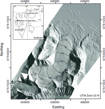
Fig. 1. Shaded relief 1 m resolution DEM of midtre Lovénbreen and surroundings derived from airborne lidar data. Inset shows location in the Kongsfjorden area of northwest Svalbard. Glacier surface contour intervals of 50 m are shown.
During the 2003 field season, lidar data and vertical stereo photography were acquired concurrently using an Optech ALTM 3033 lidar instrument and a Wild RC10 frame camera. Lidar data were collected in 2003 and again in 2005 using a scan rate of 28Hz, a laser pulse rate of 33 kHz and a scan angle of ±18 ° , resulting in along- and across-track point spacing of 1.38 and 1.33m, respectively. A swath width of ∼783 m was calculated for flat terrain at the ML mean equilibrium-line altitude (ELA) at ∼395 m a.s.l. (Reference BjørnssonBjørnsson and others, 1996).
While lidar data density varied according to scan height above the surface, topography and the presence of swath overlaps, the spatial resolution of the entire dataset was estimated to be ∼1.15 points m−2. Nineteen colour photographs at a scale of approximately 1 : 8000 were selected from the 2003 sortie total to provide adequate stereo coverage of the glacier, forefield and surrounding mountains (Fig. 2). Image diapositives were digitally scanned at a resolution of 16 μm, resulting in ground pixel sizes of ∼0.5 m, permitting DEM collection at post spacings up to 2 m, with expected vertical precision of around ±1 m (Reference Lane, James and CrowellLane and others, 2000).

Fig. 2. Relative photo frame outline locations, orientations and tiepoint positions (triangles) for the ML 2003 block set-up. Frame exposure numbers are located in the upper left corner of each photo outline.
Methods
Lidar GCPs were manually identified, extracted and measured in the following manner. First, we identified distinctive terrain points throughout all of the frames comprising the photo block, at elevations ranging from sea level at the fjord edge to the highest peaks within the imagery and at as many points adjacent to the ice surface as possible. From this initial selection we were able to identify more than 200 potential GCP locations situated on stable topography such as bedrock, rock outcrops and moraine structures.
The task of identifying coincident locations in the lidar data was facilitated by a suite of image-processing and terrain visualization tools. We first interpolated a patch of lidar data around the terrain feature (typically ∼50 × 50 m) to a high-resolution DEM using a Delaunay triangulation gridding algorithm. We then attempted to identify the precise location of the terrain point in 3-D space using terrain visualization software (Quick Terrain Modeler, Applied Imagery). In the cases where it was possible to confidently identify each distinctive terrain feature (e.g. a mountain peak or ridge point) in a shaded relief visualization of the lidar DEM, point markers were placed onto the DEM surface at the appropriate location (Fig. 3b). Each point marker was then imported into a model of the raw lidar point-cloud data (Fig. 3d), and the 3-D coordinates of the closest raw lidar point to each marker location were extracted. In those instances where shaded relief visualization of the terrain surface alone was insufficient to confidently locate the GCP, we overlaid the laser signal intensity return over the DEM surface (Fig. 3c).
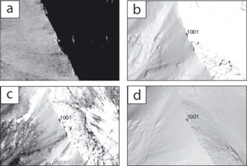
Fig. 3. GCP selection routine: point 1001 is identified in (a) vertical aerial imagery and (b) a shaded relief perspective-view lidar DEM. (c) Point identification was facilitated by overlaying the laser intensity return information onto the DEM surface; (d) raw point-cloud lidar data for the same view.
These data provided additional information with which to identify coincident points between the aerial images and the lidar elevation data, in particular when proximal to areas of very high (e.g. light snow surfaces) or low (e.g. ponded liquid water) laser reflectivity. Using these methods we were able to locate a total of 50 GCPs throughout the images comprising the photo block (Fig. 4). Three-dimensional coordinates extracted from the nearest raw lidar point to the GCP marker location were assigned to each relevant control point when measured in the aerial photographs. As some authors have reported lidar errors to increase with off-nadir scan angle (e.g. Reference BaltsaviasBaltsavias, 1999a), we selected marker locations as close as possible to the centre of each of the nine swaths comprising the full dataset. GCP extraction was therefore limited to a zone 200 m either side of the swath centre, representing 25% of the full swath width either side of the nadir point (assuming an average width of 783 m).
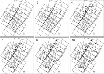
Fig. 4. GCP configurations for photogrammetric models 1, 2, 4, 6, 8 and 10 with 5, 10, 20, 30, 40 and 50 control points, respectively. Triangles represent horizontal control, circles represent vertical control and circles containing a triangle are 3-D GCPs.
To examine the effects of GCPs chosen from swath edges on DEM quality and geodetic volume change, we identified points in the central area of one swath which also lay close to the edge of an adjacent and overlapping swath (within the outer 5% of the swath width, or 40 m of the swath edge). It was then possible to alter the coordinates of GCPs from those of the closest lidar point in the centre swath to those of the closest lidar point from the edge of the overlapping swath. A total of 50 points identifiable in both the lidar data and aerial photos were selected, of which 20 were additionally identified along overlapping swath edge zones.
Standard errors were assigned to GCP coordinates based on lidar instrument manufacturer recommendations (x, y) and elevation accuracy assessment results (z, see Table 1). Standard errors of GCP coordinates allow the collinearity adjustment equations of the photogrammetric triangulation process a degree of flexibility in order to reach a solution (Reference Wolf and DeWittWolf and DeWitt, 2000). All swath-centre GCPs were assigned standard errors of ±0.5 m in x, y (Optech, 2005) and ±0.25 m in z. This estimate was based on a residual root-mean-square (RMS) error of 0.14 m between lidar elevations and check data on the ice (Table 1) and takes account of the expected lower accuracy of GCPs extracted from steeper sloping rock terrain surrounding the glacier surface. Swath edge GCPs were first assigned the same standard error as swath-centre GCPs, but were then increased to 0.5 m z to account for expected lower accuracy at swath edges. Photogrammetric model solutions were processed using both of these standard error configurations for swath-edge control points.
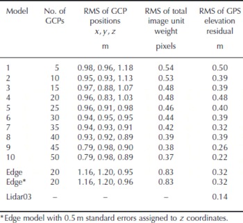
Table 1. Photogrammetric model performance: bundle adjustment of models 1–10 took place after adding five additional GCPs at each step. Elevation residuals were calculated between all the models and GPS data were collected on the days closest to airborne survey (8 August 2003 and 12 August 2003). Lidar 2003 DEM included for comparison (final row)
The effects of the addition of lidar point-derived ground control to the block adjustment were examined by setting up and then adjusting an initial block consisting of the 19 scanned images from four flight-line strips with 90 evenly distributed tie points (Fig. 2) and five GCPs (Fig. 4, model 1). The first five GCPs provided an initial solution and were positioned to include control in photos at either end of the longest image strip (photos 3041–3049, Fig. 2) and at least one GCP in each of the four strips (Fig. 4, model 1). Subsequent model solutions were derived by keeping the block and tie-point set-up constant and adding the remaining GCPs in groups of five. Each set of five additional control points were distributed evenly throughout the block where possible, and resulted in 10 individual models controlled by between 5 and 50 GCPs (Fig. 4, models 1, 2, 4, 6, 8 and 10 with 5, 10, 20, 30, 40 and 50 GCPs, respectively).
The block and tie-point set-up remained the same throughout the experiment, and a least-squares triangulation adjustment was solved for each model. We investigated the effects of GCP addition on consecutive model solutions by examining the RMS error of adjusted GCP positions and the total image unit weight (a good indicator of the quality of the entire solution). Total image unit weight provides a measure of the overall precision of control and tie-point measurements and is calculated as the RMS (in pixels) of adjusted control and tie-point residuals following the bundle adjustment (Reference Wolf and DeWittWolf and DeWitt, 2000). Lower image unit weights indicate more tightly controlled model solutions. DEMs were processed from each of the model solutions at 10 m post spacing using a triangular irregular network (TIN) data structure and an adaptive terrain extraction matching algorithm (using SocetSet software, BAE Systems), and were validated by calculating elevation residuals between each GPS check point and its spatially coincident DEM cell value.
We investigated the effects of different GCP configurations on DEM error by differencing each lidar point-controlled photogrammetric DEM (summer 2003) from a DEM derived solely from the lidar data. This gave a straightforward quality-control test whereby differences closest to zero represented the best-quality DEM surfaces. We also examined the effects of GCP configurations on estimates of glacier volume change by computing differences between photogrammetric DEMs (summer 2003) and a DEM derived from repeat survey lidar data from summer 2005, and compared these values with volume changes between 2003 and 2005 lidar-derived models. This lidar–lidar differencing was considered to be a benchmark measurement and was used to compare the performance of lidar-controlled photogrammetric models for the measurement of glacier volume change. Glacier boundaries were delineated with binary masks for both years, and we subtracted 2005 lidar elevations from each of the 2003 models. Ice-volume changes were calculated using pixel summation of difference DEMs (e.g. Reference Etzelmüller, Vatne, Ødegård and SollidEtzelmüller and others, 1993). Total volume change (ΔV) was obtained by summing the i pixel values (hi 2003 − hi 2005) between each difference DEM contained within the larger glacier surface, A (2003), and multiplying by the area l p 2 represented by each pixel (where l p is the grid spacing) expressed as:
Mean volume change ![]() averaged over the glacier surface was calculated by dividing ΔV by area A.
averaged over the glacier surface was calculated by dividing ΔV by area A. ![]() was then divided by the time between epochs to calculate mean annual volume changes
was then divided by the time between epochs to calculate mean annual volume changes ![]() .
.
Results
Experiments solving a least-squares bundle adjustment using different lidar-derived GCP configurations showed that increasing the number of GCPs resulted in a lowering of the RMS of adjusted GCP positions (Table 1). Additionally, the total image unit weight RMS decreased consistently for consecutive models, from 0.54 (model 1) to 0.37 pixels (model 10) following the measurement of an extra 45 GCPs.
Elevation residual results indicated that the addition of GCPs improved the vertical accuracy of resultant DEMs (Table 1). Although RMS reduction was not as uniform as the reductions in total image unit weights, residual RMS values were predominantly higher for the earlier (fewer GCPs) models (e.g. model 1), and lower for the latter (larger numbers of GCPs) models (e.g. models 9 and 10).
The edge models, controlled with 20 GCPs from off-nadir scan angle positions towards the outer extents of lidar data swaths (with expected lower precision), had larger RMS of GCP positions in x and y than all the other models. Adjusted z positions compared favourably with model 4, however, which had the same number of GCPs from centre-swath positions. Total image unit weight RMS for edge models, at 0.83 pixels, was poorer (higher) than all of the swath-centre GCP models. Increasing the vertical standard error of edge GCPs had no effect on total image unit weight or DEM vertical accuracy, and only a slight effect on the RMS of adjusted GCP positions.
Examples of difference DEMs between 2003 photogrammetric models 1, 2, 4, 6, 8 and 10 and a 2003 lidar-derived DEM are displayed in Figure 5. Two areas of no data coverage in the southwest tributary and the upper part of the second east tributary were present within the photogrammetric DEMs due to cloud cover during surveying and incomplete stereo coverage. There was generally good agreement between photogrammetric and lidar elevations, with differences predominantly less than ∼0.5m. However, variability was present both within and between models. Several difference DEMs revealed large positive differences (photogrammetric elevations higher than lidar elevations) in regions adjacent to the glacier backwall and in some of the higher-elevation tributary basins. Errors of 2 m or more were evident in photogrammetric DEMs in these regions, due to small patches of seasonal snow cover resulting in poor image texture.

Fig. 5. Difference DEM images between 2003 lidar-controlled photogrammetric DEMs (models, 1, 2, 4, 6, 8 and 10) and a 2003 lidar-derived DEM of midtre Lovénbreen.
While these errors remained in all models, they reduced in size throughout the later models. Snowpatches were estimated to cover less than 5% of the area of the accumulation zone at the time of survey. The DEMs with the fewest GCPs (models 1 and 2) displayed a region of large negative differences (photogrammetric elevations lower than lidar elevations) on the western side of the glacier at easting 436000–436500, northing 8758000–8759000. This apparently systematic trend was probably caused by insufficient ground control in frame 3073 of the second image strip (Fig. 4, models 1 and 2), as it was no longer evident from model 4 onwards (Fig. 5). Other examples of elevation differences of approximately ±2 m were evident at the steeply sloping (and relatively poorly textured) glacier snout for the models of fewer GCPs (1–4), and at the confluence of the large central tributary and the main glacier flow unit (easting 435500, northing 8757000) where the terrain consisted of steeply sloping, heavily crevassed ice.
The effects of lidar-controlled photogrammetric DEM error on measurements of glacier elevation change are shown in the examples in Figure 6. Errors in the photo2003–lidar2003 difference models of fewer GCPs on the west side of the glacier (Fig. 5, models 1 and 2) were manifested as relatively small elevation differences. The general pattern of elevation change in all photo models, however, was consistent with those derived from a benchmark lidar–lidar measurement (Fig. 6). Elevation changes were predominantly largest at lower elevations (at the glacier terminus), with up to 5 m of thinning, and were progressively smaller up-glacier. In comparison to the benchmark, earlier photogrammetric models (1 and 2) underestimated elevation changes at the mid-section of the glacier (northing 8758000–8759000), yet slightly overestimated changes at higher elevations (northing 8756500–8757500). This trend became less pronounced in later models (model 6 onwards, Fig. 6). Photo models 8–10 reproduced the benchmark pattern of thinning most accurately, with model 10 most resembling the overall elevation change of the lidar–lidar model. Each of the photogrammetric difference models showed small areas of large elevation change at the highest parts of the glacier. These data suggested up to 5 m of thinning whereas in the same locations in the benchmark model, thinning was predominantly less than 2.5m. This suggests that even when controlled with large numbers of GCPs, the image-matching algorithm struggled to accurately reproduce the terrain surface in these small textureless snowpatches.

Fig. 6. Midtre Lovénbreen surface elevation loss, 2003–05, measured by lidar point-controlled photogrammetric models 1, 2, 6, 8 and 10 and repeat survey lidar data. The benchmark lidar–lidar DEM differencing is included for comparison (labelled Lidar03-Lidar05).
Total volume errors (ΔV E), calculated as the difference in ice volume between each lidar point-controlled 2003 photogrammetric DEM and a lidar-only DEM from the same year, are given on the left side of Table 2. Model 1, with the fewest control points (5 GCPs), showed the largest volume error (3.37 × 10⁶ m3). Errors reduced as more GCPs were added, until models 6 and 7 (which showed the same error of 0.23×10⁶ m3). Photogrammetric models 8–10 had slightly larger volume errors but performed significantly better than models 1–3. The DEM controlled using lower-precision swath-edge GCPs performed poorly, with volume error of 3.23 × 10⁶ m3, only marginally better than model 1 despite having an additional 15 GCPs.
Table 2. Total volume errors (ΔV
E) between 2003 photogrammetric models and 2003 lidar model, and total (ΔV), area-averaged ![]() and annual area-averaged
and annual area-averaged ![]() ice volume loss at midtre Lovénbreen, 2003–05, as measured by lidar–lidar DEM differencing (Lidar03) and photogrammetry–lidar DEM differencing using 11 different GCP configurations. Values in the final column represent percentage difference in volume loss between each photogrammetric model and the lidar–lidar benchmark volume loss measurement
ice volume loss at midtre Lovénbreen, 2003–05, as measured by lidar–lidar DEM differencing (Lidar03) and photogrammetry–lidar DEM differencing using 11 different GCP configurations. Values in the final column represent percentage difference in volume loss between each photogrammetric model and the lidar–lidar benchmark volume loss measurement

Glacier volume change measurements resulting from 2003–05 DEM differencing are provided in Table 2. Comparison of photogrammetric volume changes with net glacier volume change from benchmark lidar–lidar differencing (4.72 × 10⁶ m3) showed that earlier models (1–4) overestimated volume loss by between 14% (model 3) and 53% (model 1). With the exception of model 7 (which underestimated volume loss by 27%), models 5–10 provided estimates that were within 12% of the benchmark measurement. The edge GCPs model overestimated glacier volume loss by 31%, a similar magnitude to that of model 2.
Glacier thinning and ice volume loss between 2003 and 2005 measured by lidar point-controlled photogrammetry translated to markedly different estimates of mean annual area-averaged volume loss ![]() . Differencing model 1 with 2005 repeat survey data revealed a
. Differencing model 1 with 2005 repeat survey data revealed a ![]() loss of 0.79 m a−
1. Adding 5 GCPs (model 2) reduced this value to 0.73 m a−
1, and further to 0.65ma−
1 for model 4 (20 GCPs). The best estimates of
loss of 0.79 m a−
1. Adding 5 GCPs (model 2) reduced this value to 0.73 m a−
1, and further to 0.65ma−
1 for model 4 (20 GCPs). The best estimates of ![]() were provided by models 5, 6, 9 and 10 which were all within 0.02 m a−
1 (4%) of the benchmark value, 0.51 m a−
1. The edge GCPs model overestimated mean annual area-averaged volume loss by 0.18 m a−
1 (31%).
were provided by models 5, 6, 9 and 10 which were all within 0.02 m a−
1 (4%) of the benchmark value, 0.51 m a−
1. The edge GCPs model overestimated mean annual area-averaged volume loss by 0.18 m a−
1 (31%).
Discussion
The mass loss of mountain glaciers and ice caps (MG and IC) and subsequent contribution to sea-level rise between 1993 and 2003 was 0.77 ± 0.22 mm a− 1, a rate that outweighs contributions from both the larger Greenland and Antarctic ice sheets (Reference SolomonIPCC, 2007). This large uncertainty is partly due to problems of sample size, distribution and scaling in global records of MG and IC volume change. Existing measurements must be added to, improved and extended if this uncertainty is to be reduced. Additionally, retrospective extension of the timeline of volume change studies is necessary in order to view recent rapid changes within a long-term context.
Photogrammetric processing of aerial imagery archives offers the only opportunity to remotely reconstruct direct changes in glacier volume. We have shown that high-resolution raw lidar point-cloud data collected over glaciated terrain may be used to extract large numbers of GCPs to accurately control photogrammetric models. In contrast to lowland topography, many glacial and high-mountain environments have sufficient terrain features and topographic complexity (e.g. peaks, ridges, nunataks and moraine structures) to identify conjugate points in raw point-cloud lidar data and optical imagery.
We have also shown that 3-D visualization tools and laser intensity drapes facilitate this process. Our approach provides an orientation solution that does not take account of the direct orientation of the aircraft (from GPS and INS measurements). Rather, the post-processed coordinates of individual laser pulses are used, so our approach may be readily extended to archival imagery. Providing the lidar system is well calibrated and non-moving points are identifiable, this technique may be used to reconstruct long-term volume changes without the need for field-measured ground control. Our approach replicates the standard method of controlling aerial photographs (using individual GCPs, in contrast to line- or area-based image co-registration) and is therefore more accessible to non-specialists with access to desktop photogrammetric processing software.
We designed and implemented a series of experiments to optimize the use of point-cloud lidar data as photogrammetric ground control for glacier DEMs. Increasing the number of GCPs in each model reduced the RMS of GCP positions for consecutive adjustments and reduced the total image unit weight RMS (Table 1), implying an increase in the overall quality of each solution. Addition of GCPs also increased the elevation accuracy of resultant DEMs (when compared to check data) with residual RMS of 0.50 m (model 1, 5 GCPs) reducing to 0.22 m (model 10, 50 GCPs), a value that approaches the accuracy of the lidar-only DEM (0.14 m) and is better than that predicted (Reference Lane, James and CrowellLane and others, 2000).
It is reasonable to assume from these results that the addition of ground control better constrained the model solution, reducing false image matches and minimizing erroneous elevation returns. Plots of the difference between photogrammetric models and the lidar-only DEM showed that larger false image matches (blunders) were reduced in later models (Fig. 5), a result of model adjustments being better constrained by a greater number of GCPs.
Despite the promising results of our check-data analysis plots of elevation change between photo models and the 2003 lidar model (Fig. 5) and between photo models and the 2005 lidar model (Fig. 6) showed that DEM errors of up to 2 m remained in the small snow-covered areas adjacent to the glacier backwall and higher-elevation tributaries. This was due to poor image texture and was not related to adjustment quality. This result confirms that photogrammetric elevations tend to ‘float’ in areas of poor contrast, and highlights the need for data from featureless snow cover to be treated with caution.
The RMS vertical accuracy of our DEMs was comparable to that achieved by check point analysis of photogrammetric models controlled using straight-line segments from lidar data using the same frame camera (RC-10) and a similar base-to-height ratio (standard deviation ±0.42 m) (Reference Habib, Ghanma, Kim and MitishitaHabib and others, 2004). The production of a model using GCP coordinates from sub-optimal positions (swath edges where off-nadir scanning angle is greatest, laser footprint sizes may be largest and thus laser range accuracy reduced) produced models of a lower quality and a less accurate DEM than a model using the same or fewer GCPs from optimal (swath-centre, close to nadir) locations.
These results have important implications for the measurement of glacier volume change. A benchmark measurement from lidar–lidar DEM differencing at midtre Lovénbreen between 2003 and 2005 showed that the glacier lost 4.72 × 10⁶ m3 of ice between surveys, corresponding to a mean area-averaged annual volume loss ![]() of 0.51 m a−
1. This is less negative than an estimate by Reference KohlerKohler and others (2007) of −0.69 m a−
1 for the same measurement period. The difference may be attributable to our method of differencing at the pixel level in contrast to differencing interpolated pixels between historical map contour intervals, as performed by Reference KohlerKohler and others (2007). The photogrammetric model controlled using sub-optimal swath-edge GCPs overestimated ice volume loss by 31% (Table 2). As the GPS check-data residual for this model was comparatively low (0.32 m RMS, Table 1) we may conclude that elevations were more erroneous further up-glacier where check data were limited. Similarly, we found that lidar-controlled photogrammetric models 1–4 overestimated volume loss, although the overestimates reduced as more GCPs were added to the models (Table 2). Volume loss was overestimated by between 53% (model 1) and 14% (model 3). Photogrammetric models 5, 6 and 8–10 gave estimates of mean annual area-averaged volume change which were within 0.02 m a−
1 (4%) of the benchmark measurement. Model 7, however, underestimated total volume loss by 27%, probably due to unidentified blunder errors. Given this result, we recommend that DEMs be manually checked for blunder errors to guard against the exceptions that may occur even for well-controlled block adjustments.
of 0.51 m a−
1. This is less negative than an estimate by Reference KohlerKohler and others (2007) of −0.69 m a−
1 for the same measurement period. The difference may be attributable to our method of differencing at the pixel level in contrast to differencing interpolated pixels between historical map contour intervals, as performed by Reference KohlerKohler and others (2007). The photogrammetric model controlled using sub-optimal swath-edge GCPs overestimated ice volume loss by 31% (Table 2). As the GPS check-data residual for this model was comparatively low (0.32 m RMS, Table 1) we may conclude that elevations were more erroneous further up-glacier where check data were limited. Similarly, we found that lidar-controlled photogrammetric models 1–4 overestimated volume loss, although the overestimates reduced as more GCPs were added to the models (Table 2). Volume loss was overestimated by between 53% (model 1) and 14% (model 3). Photogrammetric models 5, 6 and 8–10 gave estimates of mean annual area-averaged volume change which were within 0.02 m a−
1 (4%) of the benchmark measurement. Model 7, however, underestimated total volume loss by 27%, probably due to unidentified blunder errors. Given this result, we recommend that DEMs be manually checked for blunder errors to guard against the exceptions that may occur even for well-controlled block adjustments.
Our results illustrated the potential problems of measuring too few GCPs when generating photogrammetric estimates of glacier volume change. Each of our models featured GCPs that were well distributed throughout the photo block (Fig. 4) and at elevations ranging from the forefield (∼0–50 m a.s.l) to the glacier backwall (∼700–800 m a.s.l). However, models 1 and 2 with 5 and 10 GCPs overestimated glacier volume change by 53% and 40%, respectively.
A previous volume change study at ML generated a photogrammetric DEM from 1995 aerial photographs using just 7 GCPs which ‘due to problems of accessibility and safety’ were located in the glacier forefield alone (Reference RippinRippin and others, 2003). The authors reported a mean accuracy of 9.8 m (reduced from 23.2 m following the application of a linear regression derived correction factor) which resulted in error estimates exceeding their measured changes in volume. While it is difficult to make a direct comparison of the accuracy of the Reference RippinRippin and others (2003) DEM (due to differences in image scale and scanning resolution), it is clear that the large systematic errors, more than an order of magnitude greater than those presented in this paper, were a result of inadequate quantity and spatial distribution of GCPs. Our findings indicated that when over 20–25 well-distributed GCPs were measured, lidar raw point-controlled photogrammetry was capable of generating glacier volume change measurements within ∼4% of those derived from repeat lidar elevation data (accurate to 0.14 m RMS). Lidar data collected from insufficiently calibrated systems or with very long GPS baselines may be of lower quality, which will in turn degrade the accuracy of DEM products and volume change measurements generated using this method. Likewise, factors such as large tectonic uplift rates and vegetation cover may affect the absolute accuracy of GCP coordinates assigned to non-moving terrain points from contemporary lidar data.
Based on the findings of this work, we recommend that when deriving DEMs for glacier volume change assessment from multiple stereo photographs (in this case 19; see Fig. 2) a minimum of 20–25 (and ideally more than 40) lidar point-derived GCPs should be measured throughout the block. When this is possible, systematic elevation errors may be minimized and RMS errors reduced to approach those achievable from a lidar-derived DEM. GCPs should be measured from raw lidar data swath centres. Points remeasured using swath edge coordinates were shown to have poorer overall model solution statistics, systematic errors of up to ±2 m when compared to a lidar DEM and check data and may overestimate volume change by up to 31%.
The use of point-cloud lidar data as photogrammetric ground control has implications for optimizing the retrieval of high-quality elevation data from stereo-imagery archives and may be used to improve DEMs, and therefore glacier volume change measurements, from a variety of image sources. Similar techniques may be applied to space-borne satellite imagery from across- and along-track stereo sensors such as SPOT (Système Probatoire pour l’Observation de la Terre) or ASTER (Advanced Spaceborne Thermal Emission and Reflection Radiometer). The efficiency of our technique may be improved further through the development of automated GCP selection, extraction and measurement algorithms.
Conclusions
We have outlined a method to measure photogrammetric GCPs from raw lidar point-cloud data, thus eliminating the need to measure control in the field. This is a particular advantage in glacial environments which may be impossible to access safely by foot.
Our results showed that addition of ground control to a multi-model photogrammetric block improved the RMS positional adjustment of control points, the total image unit weight of solutions and the elevation accuracy of resultant DEMs. The best photo model (50 GCPs, RMS 0.22 m) approached the accuracy of a DEM derived solely from lidar data (RMS ±0.14 m). This meant that models with 5–20 GCPs (even when well distributed throughout the block) overestimated glacier volume loss between 2003 and 2005 by 14–53%.
Models controlled with sub-optimal lidar GCPs (chosen from swath-edge locations considered to be of lower accuracy according to known and theoretical distributions of error) may result in volume loss being overestimated by up to 31%. When more than 20–25 optimal (swath-centre) GCPs were measured in a block of 19 photographs, lidar point-controlled photogrammetry may be capable of generating glacier volume change measurements within ∼4% of those derived from repeat lidar data. These results suggested that where high-resolution laser scanning data are available, photogrammetric measurements of glacier volume change from archival image sources are achievable with accuracy and precision comparable to repeat lidar surveying.
Acknowledgements
This work was made possible by a UK Natural Environment Research Council (NERC) studentship (NER/S/A/2003/11279) and RSPSoc travel bursary awarded to N.E.B., NERC grant NE/B505203/1 awarded to T.M. and the efforts of the NERC Airborne Research and Survey Facility (ARSF). Lidar data were processed by the University of Cambridge, Unit for Landscape Modelling (ULM). GPS equipment and training were provided by the NERC Geophysical Equipment Facility (GEF), and M. King (Newcastle University) provided GAMIT-processed GPS baselines. Field and logistical support at the NERC Arctic Research Station were provided by N. Cox and B. Barrett. Three-dimensional visualization software was provided by Applied Imagery, Silver Spring, MD, USA, and SocetSet photogrammetric processing software was provided by BAE Systems. We thank H. Rott, A. Arendt and an anonymous reviewer for comments that improved the manuscript.


