


Planting dates, cultivation schedules, and herbicide application timing can improve weed control by being scheduled when weeds are most vulnerable (Menalled and Schonbeck Reference Menalled and Schonbeck2013). For example, spring preplant tillage or POST herbicide applications are more efficient when the number of emerged weeds is maximized but weed size is small. If tillage or herbicide is applied too early, only a small percentage of weeds will have emerged, whereas if either occurs too late, weeds may be too large to be vulnerable (Carey and Kells Reference Carey and Kells1995; Gunsolus Reference Gunsolus1990). Accurate weed emergence models provide a tool to optimize the timing of field operations to obtain maximum weed control (Anderson Reference Anderson1994; Forcella et al. Reference Forcella, Eradat-Oskoui and Wagner1993). Weed emergence models can also improve our understanding of abiotic factors influencing seed biology and dormancy release. For example, emergence modeling studies have provided evidence that giant ragweed seed dormancy is related to cold, moist conditions during the overwinter period, supporting previous research (Davis et al. Reference Davis, Clay, Cardina, Dille, Forcella, Lindquist and Sprague2013; Schutte et al. Reference Schutte, Regnier and Harrison2012).
Giant ragweed is one of the most competitive agricultural weeds in the midwestern United States row-crop production and has developed resistance to glyphosate and acetolactate synthase (ALS)-inhibitor herbicides (Heap Reference Heap2016; Webster et al. Reference Webster, Loux, Regnier and Harrison1994). With limited herbicide options effective for giant ragweed, proper herbicide application and mechanical weed control timing is critical for maximizing weed control efficacy (Buhler et al. Reference Buhler, Hartzler, Forcella and Gunsolus1997). Giant ragweed has been one of the earliest emerging agricultural weeds in the midwestern United States, often exhibiting a single early-season flush of emergence in early spring, with 90% emergence occurring by early June (Buhler et al. Reference Buhler, Hartzler, Forcella and Gunsolus1997; Goplen et al. Reference Goplen, Sheaffer, Becker, Coulter, Breitenbach, Behnken, Johnson and Gunsolus2017; Werle et al. Reference Werle, Sandell, Buhler, Hartzler and Lindquist2014), although some populations have developed a delayed, biphasic emergence pattern (Schutte et al. Reference Schutte, Regnier, Harrison, Schmoll, Spokas and Forcella2008). Using tillage to control early-emerging weeds not only reduces reliance on herbicides but also reduces weed population densities and allows POST herbicide applications to be made to smaller weeds, making them more effective (Sellers et al. Reference Sellers, Ferrell, MacDonald and Kline2009).
There are four publications predicting the timing of giant ragweed emergence based on concurrent weather and soil characteristics (Archer et al. Reference Archer, Forcella, Korth, Kuhn, Eklund and Spokas2006; Davis et al. Reference Davis, Clay, Cardina, Dille, Forcella, Lindquist and Sprague2013; Schutte et al. Reference Schutte, Regnier, Harrison, Schmoll, Spokas and Forcella2008; Werle et al. Reference Werle, Sandell, Buhler, Hartzler and Lindquist2014). All models base predictions on thermal time accumulation (either growing degree days [GDD] or hydrothermal time [HTT]) but use different soil temperature and moisture criteria for thermal time accumulation (Table 1). All models but Archer et al. (Reference Archer, Forcella, Korth, Kuhn, Eklund and Spokas2006) have used the soil temperature and moisture model (STM2) (Spokas and Forcella Reference Spokas and Forcella2009) to predict soil temperature and moisture, although predictions were from different soil depths. The STM2 uses site-specific soil information, daily precipitation, and minimum and maximum air temperatures from a nearby weather station to predict soil temperature. Although the STM2 model can be highly accurate, it does not account for soil shading as crop canopies develop (Perreault et al. Reference Perreault, Chokmani, Nolin and Bourgeois2013; Schutte et al. Reference Schutte, Regnier, Harrison, Schmoll, Spokas and Forcella2008).
Table 1 Published models predicting the emergence pattern of giant ragweed as cumulative percent emergence.Footnote a
a Abbreviations: c, curve shape parameter; drop, lower horizontal asymptote relative to upper asymptote; GDD, growing degree days; HTT, hydrothermal time; lrc, natural log of the rate of increase; M, upper horizontal asymptote; STM2, soil temperature and moisture model (Spokas and Forcella Reference Spokas and Forcella2009); z, HTT of first emergence.
b Models include the same fixed effects but different random effects for lrc and/or Drop determined by weather variables.
c Indicates model also includes random effects for the given parameter determined by weather variables.
For this analysis, 11 models were derived from four publications predicting giant ragweed emergence (Table 1). The single fixed-effect model from Archer et al. (Reference Archer, Forcella, Korth, Kuhn, Eklund and Spokas2006) predicts giant ragweed emergence with HTT using the Gompertz function:
 $$Y\,{\equals}\,100\,{\asterisk}\,{\rm exp}\left[ {{\minus}6{\rm }\,{\asterisk}\,{\rm exp}\left( {{\minus}0.02\,{\asterisk}\,{\rm HTT}} \right)} \right]$$
where Y is cumulative percent emergence and HTT is the predictor variable. All other published models use the Weibull function to predict giant ragweed emergence. The models from Schutte et al. (Reference Schutte, Regnier, Harrison, Schmoll, Spokas and Forcella2008) and Werle et al. (Reference Werle, Sandell, Buhler, Hartzler and Lindquist2014) include only fixed effects:
 $$Y\,{\equals}\,M\,{\asterisk}\,\left\{ {1\,{\minus}\,{\rm exp}\left[ {\left( {{\minus}\,{\rm exp}\left( {{\rm lrc}} \right)} \right)\,{\asterisk}\,\left( {{\rm GDD}\,\,{\rm or}\,\,{\rm HTT}\,{\minus}\,z} \right)\,^{\wedge} c} \right]} \right\}$$
where Y is cumulative percent emergence, M is the upper horizontal asymptote, lrc is the natural log of the rate of increase, GDD or HTT is the predictor variable, z is the time of first emergence, and c is the curve shape parameter. The fixed-effects models have model parameters that are fixed across all locations, years, and changing weather conditions, with model parameters presented in Table 1. Davis et al. (Reference Davis, Clay, Cardina, Dille, Forcella, Lindquist and Sprague2013) included an additional fixed effect for a lower horizontal asymptote (Drop) to the Weibull function, as in Equation 3:
 $$Y\,{\equals}\,M\,{\minus}\,\left( {{\rm Drop}{\plus}drop} \right)\,{\asterisk}\,{\rm exp}\left[ {\left( {{\minus}{\rm exp}\left( {{\rm lrc{\plus}}lrc} \right)} \right)\,{\asterisk}\,\left( {{\rm HTT}} \right)\,^{\wedge} \,c} \right]$$
as well as random effects for drop and lrc, which were determined by their published associations with weather variables and were different for each site-year (Equation 3). The terms for drop included by Davis et al. (Reference Davis, Clay, Cardina, Dille, Forcella, Lindquist and Sprague2013) determine how much lower the lower horizontal asymptote is relative to the upper horizontal asymptote, which had a fixed value of 99.8 for all models derived from Davis et al. (Reference Davis, Clay, Cardina, Dille, Forcella, Lindquist and Sprague2013) (Table 1). In Equation 3, Drop and drop are the fixed and random effects, respectively, for the lower horizontal asymptote relative to the upper asymptote, and lrc and lrc are the fixed and random effects, respectively, for the natural log of the rate of increase. Fixed-effect parameters for all models are presented in Table 1, while random-effect parameters were estimated from their associations with weather variables found in Davis et al. (Reference Davis, Clay, Cardina, Dille, Forcella, Lindquist and Sprague2013).
The model from Schutte et al. (Reference Schutte, Regnier, Harrison, Schmoll, Spokas and Forcella2008) was a two-part model, with a pre– and post–lag phase component based on the Weibull function, designed to predict emergence of giant ragweed with a biphasic emergence pattern like the populations found in Ohio. Both phases of this model had an HTT predictor variable but different base soil matric potential and model parameters for each phase (Table 1). Werle et al. (Reference Werle, Sandell, Buhler, Hartzler and Lindquist2014) presented two models, one of which was the best giant ragweed emergence model in their study and another which was a common model among other weed species evaluated in their study. Both models from Werle et al. (Reference Werle, Sandell, Buhler, Hartzler and Lindquist2014) were fixed-effects Weibull functions with GDD predictor variables but with different base temperatures for GDD calculation and different model parameters (Table 1).
The models from Davis et al. (Reference Davis, Clay, Cardina, Dille, Forcella, Lindquist and Sprague2013) included two mixed-effects Weibull functions with an HTT predictor variable designed for either arable or riparian accessions of giant ragweed. Each model had different fixed-effect parameters for lrc and c but the same fixed-effect parameters for M and Drop. In addition to the fixed effects, these models included random effects for lrc and drop. Davis et al. (Reference Davis, Clay, Cardina, Dille, Forcella, Lindquist and Sprague2013) found that overwinter GDD (10 C) and rainfall during seedling recruitment were both negatively associated with the random effect lrc and that rainfall during seedling recruitment was negatively associated with the random effect drop. Davis et al. (Reference Davis, Clay, Cardina, Dille, Forcella, Lindquist and Sprague2013) concluded that these weather variables are what influenced deviations from the fixed-effects-only models, and therefore can be used to improve model predictions in years or locations with differing weather conditions. The associations found by Davis et al. (Reference Davis, Clay, Cardina, Dille, Forcella, Lindquist and Sprague2013) between weather variables and random effects for lrc and drop were used to predict the random-effect parameters for each site-year of this study, which is how Models 4 to 8 were derived in Table 2. All giant ragweed populations in our study were from arable accessions, so arable accession Model 2 was used as a basis for the mixed-effects Models 4 to 8 (Tables 1 and 2). Models 4 to 8 had the same fixed effects as arable accession Model 2 but different random effects for each site-year that were predicted from Davis et al. (Reference Davis, Clay, Cardina, Dille, Forcella, Lindquist and Sprague2013).
Table 2 Summary of model performance criteria ordered by model performance across experiments and site-years (n=1,586).Footnote a
a Abbreviations: A, measure of accuracy; AICc, corrected Akaike’s information criterion; w i , Akaike weight; CCC, concordance correlation coefficient (product of r and A); GDD, growing degree days; HTT, hydrothermal time; P drop, drop determined by precipitation during recruitment; P lrc, natural log of the rate of increase determined by precipitation during recruitment; r, Pearson’s correlation coefficient; RMSE, root mean square error; W lrc, natural log of the rate of increase determined by winter GDD (10 C) from October to March.
Davis et al. (Reference Davis, Clay, Cardina, Dille, Forcella, Lindquist and Sprague2013) and Schutte et al. (Reference Schutte, Regnier, Harrison, Schmoll, Spokas and Forcella2008) developed giant ragweed emergence models by evaluating giant ragweed emergence with no surrounding vegetation, while Werle et al. (Reference Werle, Sandell, Buhler, Hartzler and Lindquist2014) developed emergence models in an experiment planted to soybean [Glycine max (L.) Merr.] that achieved a crop canopy after the majority of giant ragweed emergence had occurred. Although Schutte et al. (Reference Schutte, Regnier, Harrison, Schmoll, Spokas and Forcella2008) validated their model in both no-tillage and tilled conditions, the type of crop, crop residue, and tillage influences the soil environment, which can alter giant ragweed emergence. Since all published emergence models were constructed in either fallow or annual row-crop systems, it is likely that model performance, or how closely a model predicts actual giant ragweed emergence, will decrease in perennial crops or crops planted early in the season and in narrow rows, because they affect early-season soil temperature and moisture (Liebman and Dyck Reference Liebman and Dyck1993). Giant ragweed emergence has been shown to be prolonged with less total seedling recruitment in established alfalfa (Medicago sativa L.), which was attributed to lower soil temperatures being less conducive to giant ragweed recruitment (Goplen et al. Reference Goplen, Sheaffer, Becker, Coulter, Breitenbach, Behnken, Johnson and Gunsolus2017; Wortman et al. Reference Wortman, Davis, Schutte, Lindquist, Cardina, Felix, Sprague, Dille, Ramirez, Reicks and Clay2012). It is important to validate the applicability of giant ragweed emergence models in diverse cropping systems to identify reliable models for timing field operations. The objectives of this research were to evaluate the performance of published giant ragweed emergence models across contrasting cropping systems, and determine biotic or abiotic factors associated with deviations in emergence model predictions.
Materials and Methods
Crop Rotation Experiments
Two field experiments were initiated in 2012 and 2013 at separate sites with naturally occurring giant ragweed resistant to glyphosate and ALS-inhibitor herbicides near Rochester, MN (43.91°N, 92.56°W). Crop management details are outlined in Goplen et al. (Reference Goplen, Sheaffer, Becker, Coulter, Breitenbach, Behnken, Johnson and Gunsolus2017) and consisted of six 3-yr crop rotation treatments applied in a randomized complete block design with four replications. Crops in the rotations were corn (Zea mays L.), soybean, wheat (Triticum aestivum L.), and alfalfa. Rotations were continuous corn, soybean–corn–corn, corn–soybean–corn, soybean–wheat–corn, soybean–alfalfa–corn, and alfalfa–alfalfa–corn. Giant ragweed emergence was monitored on a weekly basis with emergence data from a total of 120 experimental units over 3 yr being used for emergence model analysis, as weekly emergence data were not collected in 2012.
Tillage Experiments
Two additional field experiments were conducted in 2015 near Rochester, MN (43.91°N, 92.56°W) and at the University of Minnesota Rosemount Research and Outreach Center near Rosemount, MN (44.70°N, 93.08°W) (Goplen Reference Goplen2017). Both sites had naturally occurring giant ragweed resistant to glyphosate, and at Rochester, MN, giant ragweed was also resistant to ALS-inhibitor herbicides. Each experiment had six tillage treatments arranged in a randomized complete block design with four replications. The tillage treatments included multiple dates of spring tillage timed relative to the initiation of giant ragweed emergence. Treatments included tillage with a field cultivator at a depth of 10 cm at emergence onset; at 14, 28, and 42 d after emergence onset; at emergence onset and repeated at 28 d after onset; and no tillage. At Rochester, MN, two replications were in oat stubble that had no fall tillage, and the other two replications were in fall chisel-plowed corn stubble. At Rosemount, MN, all replications took place in fall chisel-plowed soybean stubble. Plots at Rosemount, MN, were 3 by 6 m, and plots at Rochester, MN were 3.7 by 6 m to accommodate equipment size. Ten 0.09-m2 quadrats were placed in each plot. Giant ragweed emergence was monitored by counting and removing emerged seedlings in each quadrat on a weekly basis, starting at emergence onset and continuing for at least 10 wk or until emergence ceased. All emergence data were converted to a cumulative percentage of giant ragweed that emerged each week. These tillage timing experiments contributed data from 48 experimental units for analysis of giant ragweed emergence models.
Environmental Effects
Daily precipitation and minimum and maximum air temperatures were obtained from the National Weather Service station within 5 km of each study location. Weather data from each weather station were used to predict daily soil temperature (C) and moisture (MPa) at 1-, 2-, and 5-cm depths using STM2 (Spokas and Forcella Reference Spokas and Forcella2009). The STM2 predictions were based on daily maximum and minimum air temperature, daily precipitation, soil properties (sand, silt, clay, and organic matter), latitude, longitude, and elevation.
Thermal time for each giant ragweed emergence model was calculated using the method specified in the respective publication. All emergence models calculated GDD as:
 $${\rm GDD}\,{\equals}\,\mathop{\sum}\nolimits_{S1}^{S2} {{{ \left( {T_{{{\rm max}}} {\plus} T_{{{\rm min}}} } \right)} \over 2}{\minus}T_{{b }} } $$
where T max is maximum daily soil temperature, T min is minimum daily soil temperature, T b is base temperature for GDD calculation presented in Table 1, and S 1 and S 2 are beginning and ending dates for the specific model, respectively. For models using hydrothermal time (HTT) to predict emergence, HTT was calculated as:
 $${\rm HTT}\,{\equals}\,\mathop{\sum}\nolimits_{S1}^{S2} {\theta _{H} {\rm GDD}} $$
where GDD were calculated according to Equation 4, θ H =1 when soil matric potential was in the model’s designated interval, and θ H =0 when soil matric potential was not in the model’s designated interval (Table 1). Therefore, thermal time was only accumulated when soil moisture was in the designated interval. Soil temperature at the 5-cm depth was recorded hourly in plots from all experiments using temperature sensors (Hobo® Water Temp Pro v2, Bourne, MA). Soil temperature data from temperature sensors were used to evaluate STM2 accuracy and explore deviations from emergence predictions in crop rotation and tillage timing treatments.
Statistical Analysis
Measures of model performance in our study were based on comparison between observed and predicted values for cumulative percent emergence of giant ragweed across the entire seedling recruitment period. Corrected Akaike’s information criterion (AICc) was used to evaluate competing giant ragweed emergence models across experiments. This criterion includes a correction for sample size and is recommended in practice over traditional AIC (Anderson Reference Anderson2008; Hurvich and Tsai Reference Hurvich and Tsai1989; Sugiura Reference Sugiura1978). It is based on the minimization of maximum-likelihood criterion and is calculated as:
 $${\rm AICc}\,{\equals}\,{\minus}2{\rm log}\left( {{\scr L}\left( {\hat{\theta }} \right)\!\!\mid\!x} \right){\plus}{{2K\left( {K{\plus}1} \right)} \over {n\,{\minus}\,K\,{\minus}\,1}} $$
where the first term involves the log-likelihood of the model, given the data, while the second term penalizes a model for K additional parameters and sample size of n. Models with lower values of AICc indicate they better represent reality given the data. Akaike weights (w i ) were calculated from the AICc values for the 11 models to determine the probability that a given model is the best descriptor of reality among the candidate models. Akaike weights were calculated as:
 $$w_{i} \,{\equals}\, {{e^{{{\minus}1\!/\!2\Delta _{i} }} } \over {\sum_{r\,{\equals}\,1}^R e^{{{\minus}1\!/\!2\Delta _{r} }} }}$$
where ∆ i is the AICc difference between the top model and the ith alternative, and R is the number of candidate models (Anderson Reference Anderson2008; Burnham and Anderson Reference Burnham and Anderson2002; Hoeting et al. Reference Hoeting, Madigan, Raftery and Volinsky1999). Akaike weights (w i ) closer to 1 indicate stronger support for a candidate model given the data. This methodology has been used in previous giant ragweed emergence modeling studies to select the best-fitting predictive model while minimizing the number of parameters (Davis et al. Reference Davis, Clay, Cardina, Dille, Forcella, Lindquist and Sprague2013; Werle et al. Reference Werle, Sandell, Buhler, Hartzler and Lindquist2014).
Since AICc will rank models even if none perform well, it is recommended that additional performance criteria be used (Anderson Reference Anderson2008; Kobayashi and Salam Reference Kobayashi and Salam2000; Legates and McCabe Reference Legates and McCabe1999; Meek et al. Reference Meek, Howell and Phene2009; Tedeschi Reference Tedeschi2006). Following earlier methods (Schutte et al. Reference Schutte, Regnier, Harrison, Schmoll, Spokas and Forcella2008; Werle et al. Reference Werle, Sandell, Buhler, Hartzler and Lindquist2014), goodness of fit for each model was analyzed using root mean square error (RMSE) and the concordance correlation coefficient (CCC) to provide measures of giant ragweed emergence model precision and accuracy. The RMSE was calculated to estimate model prediction accuracy and is recommended when using AICc model selection methods (Anderson Reference Anderson2008; Legates and McCabe Reference Legates and McCabe1999; Tedeschi Reference Tedeschi2006). The RMSE is calculated as:
 $${\rm RMSE}\,{\equals}\,\sqrt {{{\sum_{i\,{\equals}\,1}^n \left( {O_{i} \,{\minus}\,P_{i} } \right)^{2} } \over n}} $$
where O i and P i are the observed and predicted values of the cumulative percentage of giant ragweed emerged, respectively, and n is the number of comparisons. The CCC was calculated as an additional model performance measure, since it provides a measure of precision and accuracy (Mitchell Reference Mitchell1997). The CCC is:
 $$CCC\,{\equals}\,rA$$
which is the product of Pearson’s correlation coefficient (r) and accuracy (A). Accuracy (A) is a bias correction factor calculated as:
 $$ A\,{\equals}\, {{4s_{x} s_{y} \,{\minus}\,r(s_{y}^{2} {\plus}s_{x}^{2} )} \over {\left( {2\,{\minus}\,r} \right)\big( {s_{y}^{2} {\plus}s_{x}^{2} } \big){\plus}\big( {{\rm \rmu }_{y} {\minus}{\rm \rmu }_{x} } \big)^{2} }}$$
where s x is mean deviation x from μ x , s y is mean deviation y from μ y , μ y is the mean of the observed values, and μ x is the mean of the model prediction. The CCC can range from −1 to 1, with values near 1 indicating better-fitting models (Meek et al. Reference Meek, Howell and Phene2009).
Deviations from the best giant ragweed emergence model were analyzed to determine whether they were associated with crop rotation or tillage treatments or with specific soil temperature conditions. Since the best giant ragweed emergence model was from a mixed-effects model, random effects were fit to the observed data using maximum-likelihood methods in each treatment and site-year as done by Davis et al. (Reference Davis, Clay, Cardina, Dille, Forcella, Lindquist and Sprague2013). Regression analyses were then performed to determine the relationship between fitted random effects, which were the dependent variables, and crop rotation and tillage treatments and observed soil temperature data. All analyses were performed using R v. 3.1.3 (R Foundation for Statistical Computing, Vienna, Austria).
Results and Discussion
Giant Ragweed Emergence
Giant ragweed emerged early in the growing season in all experiments, where on average 90% of giant ragweed emergence occurred on May 29 and June 4 in the tillage and crop rotation experiments, respectively (Goplen Reference Goplen2017; Goplen et al. Reference Goplen, Sheaffer, Becker, Coulter, Breitenbach, Behnken, Johnson and Gunsolus2017). Crop rotations with annual crops had similar giant ragweed emergence phenology, whereas emergence was slightly prolonged in established alfalfa, likely due to the prominent early-season crop canopy (Goplen et al. Reference Goplen, Sheaffer, Becker, Coulter, Breitenbach, Behnken, Johnson and Gunsolus2017). Tillage treatment reduced giant ragweed emergence the week following tillage, likely because tillage disrupted germinating seedlings and prevented them from emerging the week following tillage (Goplen Reference Goplen2017). Tillage treatments had similar levels of total giant ragweed emergence (P=0.466), however, indicating that tillage did not stimulate or suppress total giant ragweed emergence.
Model Performance
Across all experiments and site-years, giant ragweed emergence was best fit by Model 8, a mixed-effects model derived from the arable accession model of Davis et al. (Reference Davis, Clay, Cardina, Dille, Forcella, Lindquist and Sprague2013) (Tables 1 and 2). Model 8 had the lowest AICc, greatest Akaike weight (w i ), lowest RMSE, and greatest CCC among candidate models, although it was only marginally better than Model 5, indicating that it had the best fit of emergence across diverse cropping systems in this study (Table 2). Model 8 included the fixed effects specified in Table 1, and random effects determined by overwinter GDD (10 C) accumulated from October through March (Wlrc), and precipitation accumulated during seedling recruitment (P drop). The random effect W lrc included in Model 8 alters the predicted rate of emergence, with greater values indicating more rapid emergence. Davis et al. (Reference Davis, Clay, Cardina, Dille, Forcella, Lindquist and Sprague2013) found lrc to be negatively associated with overwinter GDD (10 C), meaning lrc is greater and emergence progresses more rapidly following colder overwinter periods. The more rapid progression of giant ragweed emergence following colder overwinter periods observed in this study has been shown to be related to greater dormancy loss following cold and moist conditions (Ballard et al. Reference Ballard, Foley and Bauman1996; Davis et al. Reference Davis, Clay, Cardina, Dille, Forcella, Lindquist and Sprague2013; Schutte et al. Reference Schutte, Regnier and Harrison2012). Overwinter GDD (10C) accumulated in this study ranged from 20 to 67 GDD (10 C), which was comparable to the coldest overwinter periods observed by Davis et al. (Reference Davis, Clay, Cardina, Dille, Forcella, Lindquist and Sprague2013), which ranged from 0 to 300 GDD (10 C). This resulted in more rapid emergence predictions in all site-years of our study compared with the fixed-effects-only Model 2 (Figure 1). Davis et al. (Reference Davis, Clay, Cardina, Dille, Forcella, Lindquist and Sprague2013) also found an association (r=−0.39, P=0.10) between drop and precipitation accumulated during seedling recruitment, which was used to predict drop in Model 8 (AS Davis, personal communication). The negative association between drop and precipitation during seedling recruitment indicates that smaller values for drop occur when there is greater precipitation during seedling recruitment, resulting in an extended lag phase when there is greater precipitation during seedling recruitment. Compared with Model 2, including the random effects W lrc and P drop in Model 8 improved model performance by reducing RMSE by 0.04 and increasing CCC by 0.03 (Figure 1; Table 2). The improved emergence predictions with Model 8 compared with the fixed-effects-only Model 2 confirm the findings of Davis et al. (Reference Davis, Clay, Cardina, Dille, Forcella, Lindquist and Sprague2013) that random effects for lrc and drop describe deviations from the fixed-effects-only Model 2 (Table 2).
Model 5, a mixed-effects model derived from Davis et al. (Reference Davis, Clay, Cardina, Dille, Forcella, Lindquist and Sprague2013) with fixed effects and a single random effect for W lrc, was the second best performing giant ragweed emergence model evaluated in this study. The random effect in Model 5 included the same random effect for lrc (W lrc) included in Model 8 based on overwinter GDD (10 C), but did not include the random effect for drop (P drop). Including only W lrc in Model 5 still resulted in better model performance than the fixed-effects-only Model 2 and had nearly the same measures of RMSE and CCC as the top model. Model 5 had an Akaike weight (w i ) of <0.001, however, implying that there was a low probability that it was the best among the candidate models and that it did not predict emergence as well as Model 8 (Table 2).
Models 4, 6, and 7 were also mixed-effects models derived from Davis et al. (Reference Davis, Clay, Cardina, Dille, Forcella, Lindquist and Sprague2013) for arable accessions of giant ragweed but were inferior compared with Model 8 (Table 2). Model 6 included a single random effect for drop determined by precipitation accumulated during seedling recruitment (P drop), which resulted in model performance measures only marginally better than the fixed-effects-only Model 2 (Table 2). Models 4 and 7 had a random effect for lrc determined by precipitation during seedling recruitment (P lrc), and Model 7 included an additional random effect for drop based on precipitation accumulated during seedling recruitment (P drop). Random effects for lrc and drop were determined from Davis et al. (Reference Davis, Clay, Cardina, Dille, Forcella, Lindquist and Sprague2013) by the negative associations between lrc and drop and precipitation accumulated during seedling recruitment. Among all models derived from Davis et al. (Reference Davis, Clay, Cardina, Dille, Forcella, Lindquist and Sprague2013), the two best-fitting models across our experiments included a random effect for lrc determined by overwinter GDD (Models 5 and 8), while the worst-fitting models determined the random effect for lrc by precipitation accumulated during seedling recruitment (Models 4 and 7). These findings indicate that lrc is more closely associated with overwinter GDD (10 C) than precipitation during seedling recruitment (Table 2). Random-effect model parameters based on overwinter GDD (10 C) are also easier to use in making real-time emergence predictions, because random effects predicted from overwinter GDD (10 C) are known prior to giant ragweed recruitment. Random-effect parameters based on precipitation during the seedling recruitment period are unknown until the end of seedling recruitment, meaning real-time emergence predictions will require recalculation of random-effect parameters as precipitation accumulates or use of historical averages and weather forecasts to predict random-effect parameters.
Model 9 was derived to model emergence of giant ragweed with a biphasic emergence pattern in Ohio (Schutte et al. Reference Schutte, Regnier, Harrison, Schmoll, Spokas and Forcella2008) and was among the top-performing models in our study. In our study, giant ragweed emergence generally occurred after the early flush but before the late flush of emergence predicted by Model 9. This monophasic emergence pattern aligning between the two flushes of emergence predicted by Model 9 indicates that giant ragweed populations in Minnesota have not diverged in their emergence timing as populations found in Ohio have done (Figure 1).
Across the crop rotation and tillage timing experiments, soil temperature at the 5-cm depth predicted by the STM2 was associated with observed soil temperature (R2=0.88, P<0.001) (Figure 2). Although the observed and predicted soil temperatures were associated, the STM2 had a mean bias of 2.9C, indicating that the STM2 predicted soil temperature to be 2.9C warmer on average than what was observed. The 2.9C bias of STM2 temperature predictions caused predicted thermal time to accumulate faster than what actually occurred and contributed to premature giant ragweed emergence predictions for Models 1, 3, 10, and 11 in all site-years (Figure 1). This finding is similar to that of Perreault et al. (Reference Perreault, Chokmani, Nolin and Bourgeois2013), who reported a mean bias of 2.5C for STM2 on loamy soils similar to soils at both of our study locations. The mean bias of the STM2 among crop rotation and tillage timing treatments ranged from 1.7 to 3.9C. Established alfalfa and wheat had the greatest mean bias values of 3.8 and 3.9C, respectively, while soybean planted into soybean stubble had the lowest mean bias value of 1.7C. The STM2 does not account for changes in crop canopy during the growing season (Perreault et al. Reference Perreault, Chokmani, Nolin and Bourgeois2013), which likely explains why the STM2 predictions had a greater bias in established alfalfa and wheat, which were established earlier and in narrower rows compared with corn and soybean. The STM2 model was likely more accurate in previous giant ragweed emergence modeling studies, since they were developed with little or no canopy coverage (Archer et al. Reference Archer, Forcella, Korth, Kuhn, Eklund and Spokas2006; Davis et al. Reference Davis, Clay, Cardina, Dille, Forcella, Lindquist and Sprague2013; Schutte et al. Reference Schutte, Regnier, Harrison, Schmoll, Spokas and Forcella2008; Werle et al. Reference Werle, Sandell, Buhler, Hartzler and Lindquist2014). Including a 2.9C mean bias correction factor for STM2 predictions decreased the RMSE of Models 1, 3, 10, and 11 by 0.06, 0.03, 0.09, and 0.08, respectively. However, including the mean bias correction factor increased the RMSE of Model 8 by 0.02, indicating that Model 8 without a bias correction was still the best among all models evaluated.
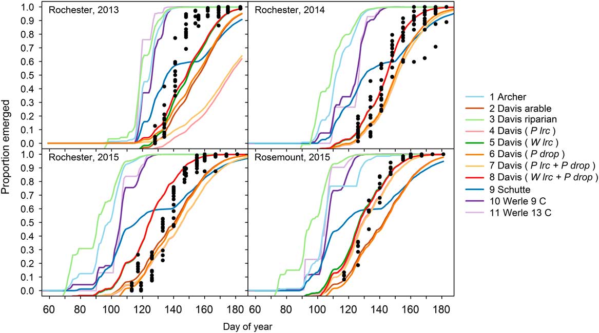
Figure 1 Predicted cumulative giant ragweed emergence by model in relation to observed mean cumulative emergence in each experimental treatment. Random effects included in the Davis et al. (Reference Davis, Clay, Cardina, Dille, Forcella, Lindquist and Sprague2013) arable-accession mixed-effects models are shown in parentheses. Abbreviations: P drop, drop determined by precipitation during recruitment; P lrc, natural log of the rate of increase determined by precipitation during recruitment; W lrc, natural log of the rate of increase determined by winter GDD (10 C) accumulated from October to March.

Figure 2 Daily average soil temperature at the 5-cm depth predicted by the soil temperature and moisture model (STM2) during the crop rotation and tillage timing experiments relative to observed soil temperature. The solid 1:1 line (y=x) indicates perfect agreement between observed and predicted soil temperature, while the dotted line indicates the fitted regression equation (y=0.96x − 2.1, R2=0.88, P<0.001) between observed and predicted soil temperature.
Soil Temperature Associations
The mixed-effects models derived by Davis et al. (Reference Davis, Clay, Cardina, Dille, Forcella, Lindquist and Sprague2013) provide a versatile framework to study giant ragweed emergence, since unexplained model deviations can be attributed to environmental variation (Luschei and Jackson Reference Luschei and Jackson2005). The associations found by Davis et al. (Reference Davis, Clay, Cardina, Dille, Forcella, Lindquist and Sprague2013) allowed the derivation of mixed-effects Models 4 through 8 in our study. Using this same approach, new estimates of the random effects drop and lrc were determined for the arable accession model (Model 2) from Davis et al. (Reference Davis, Clay, Cardina, Dille, Forcella, Lindquist and Sprague2013) for each site-year and treatment combination in our study. Regression analyses were performed to determine associations between random effects and experimental treatments and soil temperature (average daily minimum, maximum, mean, and fluctuation in temperature for various intervals during the seedling recruitment period). Neither crop rotation sequence nor tillage timing treatments were associated with the estimated random effects drop or lrc (R2=0.07 to 0.42, P=0.55 to 0.99). There also were no associations between the estimated random effects for lrc and soil temperature variables (R2=0.01 to 0.07, P=0.17 to 0.99). All soil temperature variables analyzed were positively associated with the estimated random effects for drop (R2=0.24 to 0.72, P<0.001 to 0.006), meaning warmer soil temperature variables or greater temperature fluctuations had greater fitted random effects for drop. The soil temperature variable most strongly associated with the fitted random effect for drop was the maximum daily soil temperature during the entire seedling recruitment period (R2=0.72, P<0.001). This relationship indicates that greater maximum soil temperatures during seedling recruitment were associated with greater fitted random effects for drop, the term representing the lower horizontal asymptote of the Weibull function (Figure 3). A greater random effect for drop equates to a shorter lag period at the start of giant ragweed emergence.
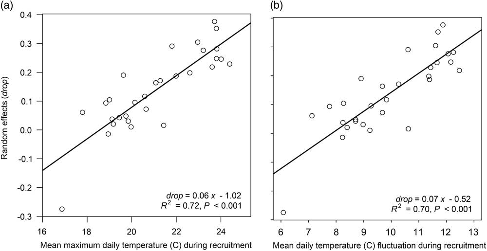
Figure 3 Association between the estimated random effects of drop and (a) mean maximum daily temperature observed at a 5-cm soil depth during the seedling recruitment period and (b) mean daily temperature fluctuation at a 5-cm soil depth during seedling recruitment.
Observed average daily soil temperature fluctuation during the entire seedling recruitment period was the second most significant association with the estimated random effects for drop (R2=0.70, P<0.001) (Figure 3). It is possible that either the amplitude or number of temperature fluctuations influences giant ragweed emergence rather than maximum soil temperature, as shown for other weed species including johnsongrass [Sorghum halpense (L.) Pers.] and large crabgrass [Digitaria sanguinalis (L.) Scop.] (Benech Arnold et al. Reference Benech Arnold, Ghersa, Sanchez and Insausti1990a, Reference Benech Arnold, Ghersa, Sanchez and Insausti1990b; Forcella et al. Reference Forcella, Benech-Arnold, Sanchez and Ghersa2000; King and Oliver Reference King and Oliver1994). Daily maximum soil temperature was the primary factor influencing daily temperature fluctuation, as evidenced by the strong association between the two variables (r=0.98, P<0.001), indicating that greater daily maximum soil temperature is more influential on daily soil temperature fluctuation than daily minimum soil temperature, which has been reported previously (Perreault et al. Reference Perreault, Chokmani, Nolin and Bourgeois2013). These findings indicate that giant ragweed emergence will have a shorter lag phase at the start of emergence in environments with greater maximum daily soil temperature and corresponding greater soil temperature fluctuation. Davis et al. (Reference Davis, Clay, Cardina, Dille, Forcella, Lindquist and Sprague2013) stated that the associations they found between random effects for lrc and precipitation accumulated during seedling recruitment may have been caused by increased cloud cover accompanying increased precipitation. Cloud cover and precipitation can limit maximum daily soil temperature, and since soil temperature was not directly measured in Davis et al. (Reference Davis, Clay, Cardina, Dille, Forcella, Lindquist and Sprague2013), it is possible that the association between random effects and precipitation during seedling recruitment found in Davis et al. (Reference Davis, Clay, Cardina, Dille, Forcella, Lindquist and Sprague2013) was driven by maximum daily soil temperature or daily temperature fluctuation, as found in the present study.
The positive association between random effects for drop and mean maximum daily soil temperature supports the findings of Goplen et al. (Reference Goplen, Sheaffer, Becker, Coulter, Breitenbach, Behnken, Johnson and Gunsolus2017), in which giant ragweed emergence extended later into the growing season in established alfalfa compared with annual crops. The extended emergence was likely due to lower soil temperatures causing a longer initial lag period in emergence. Longer initial lag periods in emergence could also be expected in other crops established early in the growing season that limit soil temperature, such as small grains or cover crops (Zhang et al. Reference Zhang, Lovdaul, Grip, Tong, Yang and Wang2009), although this was not shown to be the case for wheat (Goplen et al. Reference Goplen, Sheaffer, Becker, Coulter, Breitenbach, Behnken, Johnson and Gunsolus2017). It is also possible that crop management practices maintaining increased soil residue associated with conservation tillage will have similar effects on giant ragweed emergence, since they can also affect soil temperature (Griffith et al. Reference Griffith, Mannering, Galloway, Parsons and Richey1973; Kladivko et al. Reference Kladivko, Griffith and Mannering1986).
Model 8, a mixed-effects model derived from Davis et al. (Reference Davis, Clay, Cardina, Dille, Forcella, Lindquist and Sprague2013) that included random effects for drop and lrc based on precipitation accumulated during seedling recruitment and overwinter GDD (10C), respectively, was the model that most accurately predicted giant ragweed emergence across crop rotations and spring tillage dates. The top four models that best fit giant ragweed emergence in the present study originated from Davis et al. (Reference Davis, Clay, Cardina, Dille, Forcella, Lindquist and Sprague2013), with the top two models including random effects predicted by overwinter GDD (10 C). This is supported by studies of giant ragweed seed dormancy, which have found that cold and moist conditions during winter enhance seed dormancy release (Ballard et al. Reference Ballard, Foley and Bauman1996; Schutte et al. Reference Schutte, Regnier and Harrison2012).
This is the first study to verify the utility of previously published giant ragweed emergence models under a diversity of crop management practices and supports previous research showing that giant ragweed emergence is affected by winter weather. This research also suggests that crops such as alfalfa, small grains, and cover crops, which have lower soil temperature during seedling recruitment compared with annual row crops, will have a longer lag phase at the initiation of giant ragweed emergence, potentially extending emergence later into the growing season. The delay in emergence may provide weed control benefits, as later-emerged giant ragweed will be subjected to increased competition with established crops. As herbicide-resistant giant ragweed continues to be problematic, robust emergence model predictions will be increasingly important to optimize planting, tillage, and herbicide application dates in a variety of crop management systems to improve giant ragweed control.
Acknowledgments
This research was funded by the Monsanto Graduate Fellowship, the Rapid Agricultural Response Fund of the University of Minnesota Agricultural Experiment Station, and the Torske Klubben Graduate Fellowship. The authors express appreciation to numerous faculty, staff members, and students for their assistance, in particular Adam Davis, Brad Kincaid, Doug Miller, and Frank Forcella.


 Open access