


Co-twin control (CTC) or discordant twin models are a special case of what are commonly referred to as between-within models (Begg & Parides, Reference Begg and Parides2003; Carlin et al., Reference Carlin, Gurrin, Sterne, Morley and Dwyer2005; McGue et al., Reference McGue, Osler and Christensen2010). CTC models make use of the genetic and environmental relationships within twin-pairs to estimate an exposure effect controlling for all factors shared within a pair. Monozygotic (MZ) twins share all genetic factors and rearing environment, so any difference in outcome must be due to factors not shared within the twin-pair. If an exposure has a causal effect on an outcome, the outcome levels will differ within exposure discordant twin-pairs. In this way, the unexposed twin acts as the counterfactual to their exposed co-twin; they are an approximation of what the twin would have looked like had they not been exposed. The same logic can be extended to genetic relationships other than twins, as in sibling comparison designs (Lahey & D’Onofrio, Reference Lahey and D’Onofrio2010).
The power in the CTC design lies in its ability to implicitly control for all factors shared within a twin-pair even when they are unmeasured (McGue et al., Reference McGue, Osler and Christensen2010). For this reason, CTC designs are widely used as a stronger method of causal inference than using genetically unrelated individuals (Donovan & Susser, Reference Donovan and Susser2011). Examples of their use range from the effects of cannabis on intelligence (Jackson et al., Reference Jackson, Isen, Khoddam, Irons, Tuvblad, Iacono and Baker2016) and educational attainment (Meier et al., Reference Meier, Caspi, Danese, Fisher, Houts, Arseneault and Moffitt2018; Verweij et al., Reference Verweij, Huizink, Agrawal, Martin and Lynskey2013) to alcohol’s effect on stroke risk (Kadlecová et al., Reference Kadlecová, Andel, Mikulík, Handing and Pedersen2015) or hippocampal volume (Wilson et al., Reference Wilson, Malone, Hunt, Thomas and Iacono2018) and to how lifestyle factors influence cancer risk (Hübinette et al., Reference Hübinette, Lichtenstein, Ekbom and Cnattingius2001; Milán et al., Reference Milán, Verkasalo, Kaprio and Koskenvuo2003; Swerdlow et al., Reference Swerdlow, De Stavola, Swanwick, Mangtani and Maconochie1999). Despite the increasing popularity of the CTC design, it has not been fully explored methodologically. Work by Frisell and colleagues has shown that bias can be introduced in the CTC estimates in the presence of nonshared confounding (Frisell et al., Reference Frisell, Öberg, Kuja-Halkola and Sjölander2012). The magnitude of this bias is a function of the within-twin-pair correlation in the exposure and the confounder. This work also shows that measurement error in the exposure will bias the CTC estimate toward the null.
The current study builds on these findings by testing whether the inclusion of a measured covariate can counteract the nonshared confounding bias. In other words, can the bias induced by a nonshared confounder be reduced when a measured covariate is included in the CTC model? Incorporating potential confounders as covariates in a regression model is a popular way of controlling for confounding bias (Greenland & Morgenstern, Reference Greenland and Morgenstern2001). If the covariate is a perfect measure of the confounder, doing so will eliminate all confounding bias. Most often, however, the covariate measures the confounder with some error, resulting in residual confounding bias (Becher, Reference Becher1992). Using analytic derivations and simulations, we investigate whether covariate inclusion will reduce the bias in the CTC model estimates more than in a model treating the twins as individuals and explore what parameters affect the bias reduction in this scenario. Lastly, the impact of measurement error in not only the exposure, but also the measured covariate, is investigated. The interpretation of CTC model estimates is discussed in light of our findings.
Co-Twin Control Model
A generalized linear regression model, treating twins as individuals (the individual-level model), is given by
 $$g\left\{ {E\left( {{Y_{ij}}{\rm{|}}{X_{ij}}} \right)} \right\} = {\beta _0} + \;\beta {X_{ij}},$$
where Xij is the exposure of person j in twin-pair i, Yij is their outcome and g{ } is a link function allowing the generalized linear model to be extended to different forms of regression, like linear or logistic regression. For example, in a linear regression model, Y follows a normal distribution with the identity link function (g{μ} = μ).
The CTC model decomposes the exposure effect from the individual-level model (β) into a within-twin-pair and between-twin-pair effect by incorporating the twin-pair mean. The CTC model is given as
 $$g\left\{ {E\left( {{Y_{ij}}{\rm{|}}{X_{ij}},{{\overline X}_i}} \right)} \right\} = {\beta _0} + {\beta _W}\left( {{X_{ij}} - {{\overline X}_i}} \right) + {\beta _B}{\overline X_i},$$
where ${\overline X_i}$
is the mean exposure of twin-pair i. The within-twin-pair estimate (βW
) is the estimate of the exposure effect controlling for all genetic and shared environmental factors. The between-twin-pair estimate (βB
) is an estimate of the magnitude of confounding due to shared factors. In general, the within-twin-pair effect is of more interest to researchers than the between-pair effect.
${\overline X_i}$
is the mean exposure of twin-pair i. The within-twin-pair estimate (βW
) is the estimate of the exposure effect controlling for all genetic and shared environmental factors. The between-twin-pair estimate (βB
) is an estimate of the magnitude of confounding due to shared factors. In general, the within-twin-pair effect is of more interest to researchers than the between-pair effect.
Interpretation of the within-pair effect is commonly made by comparing βW
from the CTC model to β from the individual-level model (McGue et al., Reference McGue, Osler and Christensen2010). When these estimates are not significantly different from one another, β = βW
, this would suggest that the observed association is not due to confounding factors, consistent with a causal effect of exposure on outcome. When βW
is significantly different from β but is not 0, $\beta \ne {\beta _W} \gt 0$
, this suggest that the observed association is partially due to confounding factors. And, finally, when the within-pair effect is not significantly different from 0, βW
= 0, this would suggest that the entire association is due to confounding and is not consistent with a causal interpretation.
$\beta \ne {\beta _W} \gt 0$
, this suggest that the observed association is partially due to confounding factors. And, finally, when the within-pair effect is not significantly different from 0, βW
= 0, this would suggest that the entire association is due to confounding and is not consistent with a causal interpretation.
Bias Due to Nonshared Confounding
Prior statistical analysis of CTC models by Frisell et al. (Reference Frisell, Öberg, Kuja-Halkola and Sjölander2012) has shown that bias is induced in the within-twin-pair estimate in the presence of factors that are not perfectly shared within a twin-pair. Environmental confounding within-twin-pairs will increase bias in the within-twin-pair term as a function of the degree to which such confounding reflects influences that are unshared within a pair. If all confounding variables are perfectly shared within a twin-pair, the estimate of the effect of the exposure (βW
) will be unconfounded. As the correlation between confounding variables decreases within a twin-pair, the estimate of the effect of the exposure (βW
) will be biased upward. In some cases, this bias will exceed that of the individual-level effect $\left( \beta \right)$
. To illustrate this, we assume that the confounding variable affects both the exposure and the outcome, but that the exposure does not have a causal effect on the outcome. If we select twin-pairs in which the members of the pair are discordant on the exposure, they will also likely be more discordant on the confounding variable than unselected twin-pairs (the correlation of the confounding variable between members of a pair will be reduced). This will in turn increase the correlation between the confounder and the exposure variables and create a spurious relationship between the exposure and the outcome. The impact of nonshared confounders on the bias of β and βW
depends on the ratio of the within-pair correlation of the confounding variable
$\left( \beta \right)$
. To illustrate this, we assume that the confounding variable affects both the exposure and the outcome, but that the exposure does not have a causal effect on the outcome. If we select twin-pairs in which the members of the pair are discordant on the exposure, they will also likely be more discordant on the confounding variable than unselected twin-pairs (the correlation of the confounding variable between members of a pair will be reduced). This will in turn increase the correlation between the confounder and the exposure variables and create a spurious relationship between the exposure and the outcome. The impact of nonshared confounders on the bias of β and βW
depends on the ratio of the within-pair correlation of the confounding variable $\left( {{\rho _C}} \right)$
to the within-pair correlation of the exposure variable
$\left( {{\rho _C}} \right)$
to the within-pair correlation of the exposure variable $\left( {{\rho _X}} \right)$
. If the within-pair correlation in the confounder is greater than the within-pair correlation in the exposure, the within-twin-pair term is less biased than the individual-level term (if
$\left( {{\rho _X}} \right)$
. If the within-pair correlation in the confounder is greater than the within-pair correlation in the exposure, the within-twin-pair term is less biased than the individual-level term (if ${\rho _C} \gt {\rho _X}$
then
${\rho _C} \gt {\rho _X}$
then $bias\left( {{\beta _W}} \right) \lt bias\left( \beta \right)$
). If the correlation between confounders is less than the correlation between exposure, the within-twin-pair term is more biased than the individual-level term (if
$bias\left( {{\beta _W}} \right) \lt bias\left( \beta \right)$
). If the correlation between confounders is less than the correlation between exposure, the within-twin-pair term is more biased than the individual-level term (if ${\rho _C} \lt {\rho _X}$
then
${\rho _C} \lt {\rho _X}$
then $bias\left( {{\beta _W}} \right) \gt bias\left( \beta \right)$
). If the correlations are equal, both estimates will have the same amount of bias. Unless
$bias\left( {{\beta _W}} \right) \gt bias\left( \beta \right)$
). If the correlations are equal, both estimates will have the same amount of bias. Unless ${\rho _C} = 1$
, however, bias will always exist in the within-pair estimate (Frisell et al., Reference Frisell, Öberg, Kuja-Halkola and Sjölander2012).
${\rho _C} = 1$
, however, bias will always exist in the within-pair estimate (Frisell et al., Reference Frisell, Öberg, Kuja-Halkola and Sjölander2012).
Additionally, random measurement error in the exposure can lead to twin-pairs being incorrectly classified as concordant or discordant, which is important given that only discordant twin-pairs are informative for the within-pair effect in CTC models. As measurement error increases, the within-twin-pair estimate increasingly underestimates the true effect. Both biases due to confounding and measurement error affect the estimates from CTC models as well as more general between-within models (i.e., any models in which an exposure–outcome relationship is decomposed into a within- and between-cluster effect).
Inclusion of a Measured Covariate to Reduce Bias
While nonshared confounding may induce bias in the within-twin-pair effect, most researchers attempt to control for this by including covariates in the CTC regression model. The rationale is that the covariates incorporated into the model are an imperfect measure of unmeasured confounding variables, and by controlling them, bias due to confounding is thereby reduced. Figure 1 shows a causal diagram for one twin-pair where the exposure–outcome relationship is confounded by an unmeasured variable, C, that also affects the measured covariate, Z.

Fig. 1. Causal diagram shown for one twin-pair (subscripts of 1 and 2 represent each twin). Variables X, Y and C represent the exposure, outcome and unmeasured confounder, respectively. Z represents the measured covariate. ${\beta _{YX}}$
is the true causal effect of exposure on outcome.
${\beta _{YX}}$
is the true causal effect of exposure on outcome. ${\rm{\;}}{\beta _{ZC}}$
is the effect of the confounder on the covariate. Double-headed arrows represent familial factors that cause aggregation of phenotypes within families.
${\rm{\;}}{\beta _{ZC}}$
is the effect of the confounder on the covariate. Double-headed arrows represent familial factors that cause aggregation of phenotypes within families.
A standard way to include covariates in CTC models is given by
 $$g\left\{ {E\left( {{Y_{ij}}{\rm{|}}{X_{ij}}, {{\overline X}_i},{Z_{ij}}} \right)} \right\} = {\beta _0} + {\beta _W}\left( {{X_{ij}} - {{\overline X}_i}} \right) + {\beta _B}{\overline X_i} + {\beta _Z}{Z_{ij}},$$
where Z is the measured covariate. Sjölander et al. (Reference Sjölander, Frisell and Öberg2012), however, show that this model specification does not properly adjust for the covariate and causes βW
to lose its causal interpretation. Briefly, by conditioning on ${\overline X_i}$
, a spurious association is induced between the exposure of twin 1
${\overline X_i}$
, a spurious association is induced between the exposure of twin 1 $\left( {{X_{i1}}} \right)$
and the covariate of their co-twin
$\left( {{X_{i1}}} \right)$
and the covariate of their co-twin $\left( {{Z_{i2}}} \right)$
and between the outcome of twin 1
$\left( {{Z_{i2}}} \right)$
and between the outcome of twin 1 $\left( {{Y_{i1}}} \right){\rm{\;}}$
and the covariate of twin 2
$\left( {{Y_{i1}}} \right){\rm{\;}}$
and the covariate of twin 2 $\left( {{Z_{i2}}} \right)$
. Essentially,
$\left( {{Z_{i2}}} \right)$
. Essentially, ${Z_{i2}}$
becomes a collider variable, a common effect of two or more variables (Greenland, Reference Greenland2003), and an artificial confounder of the exposure–outcome relationship. Given this model specification, even in the absence of a true causal effect
${Z_{i2}}$
becomes a collider variable, a common effect of two or more variables (Greenland, Reference Greenland2003), and an artificial confounder of the exposure–outcome relationship. Given this model specification, even in the absence of a true causal effect ${\beta _{YX}} = 0$
, βW
will not equal 0. The authors show that a simple modification of the model can recapture the causal interpretation of βW
:
${\beta _{YX}} = 0$
, βW
will not equal 0. The authors show that a simple modification of the model can recapture the causal interpretation of βW
:
 $${g\left\{ {E\left( {{Y_{ij}}{\rm{|}}{X_{ij}},{{\overline X}_i},{Z_{ij}},{{\overline Z}_i}} \right)} \right\} = {\beta _0} + {\beta _W}\left( {{X_{ij}} - {{\overline X}_i}} \right) + {\beta _B}{\overline X_i} + {\beta _Z}\left( {{Z_{ij}} - {{\overline Z}_i}} \right),}$$
where ${\overline Z_i}$
is the mean covariate value of twin-pair
${\overline Z_i}$
is the mean covariate value of twin-pair $i$
(Sjölander et al., Reference Sjölander, Frisell and Öberg2012). The current study explores both forms of covariate inclusion to evaluate whether confounding bias can be reduced, with particular interest in bias reduction in βW
. We focus on whether, or to what extent, bias remains in the within-pair estimate even if the causal interpretation is retained as in equation 4.
$i$
(Sjölander et al., Reference Sjölander, Frisell and Öberg2012). The current study explores both forms of covariate inclusion to evaluate whether confounding bias can be reduced, with particular interest in bias reduction in βW
. We focus on whether, or to what extent, bias remains in the within-pair estimate even if the causal interpretation is retained as in equation 4.
Bias Reduction with a Covariate under a Linear Model
Assuming that all effects in the causal diagram (Figure 1) are linear and that all variables are continuous, we are able to derive the exact mathematical formula for the regression coefficients. We further assume, without loss of generality, that all variables other than error terms are standardized (a mean of 0 and a standard deviation of 1). We can then ignore the intercept term so that the true causal model is given by
 $${Y_{ij}} = {\beta _{YX}}{X_{ij}} + {\beta _{YC}}{C_{ij}} + {\varepsilon _{{Y_{ij}}}},$$
 $${X_{ij}} = {\beta _{XC}}{C_{ij}} + {\varepsilon _{{X_{ij}}}},$$
 $${Z_{ij}} = {\beta _{ZC}}{C_{ij}} + {\varepsilon _{{Z_{ij}}}}.$$
With this data-generating structure, all confounding between X and Y is due to C, with Z being a measure of C that has no direct effect on X or Y. We let ${\rm{var}}\left( C \right) = \sigma _C^2 = 1$
,
${\rm{var}}\left( C \right) = \sigma _C^2 = 1$
, ${\mathop{\rm var}} ({\varepsilon _{{Y_{ij}}}}) = \sigma _{{Y_{ij}}}^2$
,
${\mathop{\rm var}} ({\varepsilon _{{Y_{ij}}}}) = \sigma _{{Y_{ij}}}^2$
, ${\mathop{\rm var}} ({\varepsilon _{{X_{ij}}}}) = \sigma _{{X_{ij}}}^2$
and
${\mathop{\rm var}} ({\varepsilon _{{X_{ij}}}}) = \sigma _{{X_{ij}}}^2$
and ${\mathop{\rm var}} ({\varepsilon _{{Z_{ij}}}}) = \sigma _{{Z_{ij}}}^2$
. Because the causal diagram assumes twin-pairs, we have
${\mathop{\rm var}} ({\varepsilon _{{Z_{ij}}}}) = \sigma _{{Z_{ij}}}^2$
. Because the causal diagram assumes twin-pairs, we have ${\rm{cov}}\left( {{C_{i1}},{C_{i2}}} \right) \!= \!{\rho _C}\sigma _C^2$
,
${\rm{cov}}\left( {{C_{i1}},{C_{i2}}} \right) \!= \!{\rho _C}\sigma _C^2$
, ${\rm{cov}}\left( {{\varepsilon _{{Y_{i1}}\!}},{\varepsilon _{{Y_{i2}}}}} \right) = {\rho _{{\varepsilon _Y}}}\sigma _{{\varepsilon _Y}}^2$
,
${\rm{cov}}\left( {{\varepsilon _{{Y_{i1}}\!}},{\varepsilon _{{Y_{i2}}}}} \right) = {\rho _{{\varepsilon _Y}}}\sigma _{{\varepsilon _Y}}^2$
, ${\rm{cov}}\left( {{\varepsilon _{{X_{i1}}}},{\varepsilon _{{X_{i2}}}}} \right) = {\rho _{{\varepsilon _X}}}\sigma _{{\varepsilon _X}}^2$
and
${\rm{cov}}\left( {{\varepsilon _{{X_{i1}}}},{\varepsilon _{{X_{i2}}}}} \right) = {\rho _{{\varepsilon _X}}}\sigma _{{\varepsilon _X}}^2$
and ${\rm{cov}}\left( {{\varepsilon _{{Z_{i1}}}},{\varepsilon _{{Z_{i2}}}}} \right) = {\rho _{{\varepsilon _Z}}}\sigma _{{\varepsilon _Z}}^2$
. Furthermore, we make the assumptions that each twin’s error terms (ϵ) are independent of all other variables and there is no correlation between the error terms of different variables within a twin-pair.
${\rm{cov}}\left( {{\varepsilon _{{Z_{i1}}}},{\varepsilon _{{Z_{i2}}}}} \right) = {\rho _{{\varepsilon _Z}}}\sigma _{{\varepsilon _Z}}^2$
. Furthermore, we make the assumptions that each twin’s error terms (ϵ) are independent of all other variables and there is no correlation between the error terms of different variables within a twin-pair.
We are interested in the true causal effect of X on Y $\left( {{\beta _{YX}}} \right)$
. Regressing Y on X and C would result in an unbiased estimate of the exposure effect. However, C is unmeasured and leaving it out results in a biased estimate of the exposure effect. We explore the bias when regressing Y on X and Z instead. Because Z is a measure of C, including it in the regression model may reduce the confounding bias induced by the unmeasured confounder C. Furthermore, we are interested in whether the inclusion of Z reduces the bias more for the within-twin-pair effect (βW
) than the individual-level effect
$\left( {{\beta _{YX}}} \right)$
. Regressing Y on X and C would result in an unbiased estimate of the exposure effect. However, C is unmeasured and leaving it out results in a biased estimate of the exposure effect. We explore the bias when regressing Y on X and Z instead. Because Z is a measure of C, including it in the regression model may reduce the confounding bias induced by the unmeasured confounder C. Furthermore, we are interested in whether the inclusion of Z reduces the bias more for the within-twin-pair effect (βW
) than the individual-level effect $\left( \beta \right)$
.
$\left( \beta \right)$
.
Confounding Bias with Covariate Inclusion
The derived estimate of the exposure effect from the individual-level model without adjusting for a covariate (equation 1) is
 $${\beta = {\beta _{YX}} + {\beta _{YC}}{\beta _{XC}}\;.}$$
The derived estimate of the exposure effect from the CTC model without adjusting for a covariate (equation 2) is
 $${{{\beta _W} = {\beta _{YX}}} + {{{{\beta _{YC}}{\beta _{XC}}}}\over\matrix{{{\left( {1 - {\rho _{{\varepsilon _X}}}}\over{1 - {\rho _C}} \right)}}}}.$$
The full derivation steps can be found in Frisell et al. (Reference Frisell, Öberg, Kuja-Halkola and Sjölander2012). It is clear that both estimates are a function of the true causal effect $\left( {{\beta _{YX}}} \right)$
plus a bias term. Because the within-twin-pair correlation in the exposure,
$\left( {{\beta _{YX}}} \right)$
plus a bias term. Because the within-twin-pair correlation in the exposure, ${\rho _X}$
, is a linear combination of
${\rho _X}$
, is a linear combination of ${\rho _{{\varepsilon _X}}}$
and
${\rho _{{\varepsilon _X}}}$
and ${\rho _C}$
(i.e.,
${\rho _C}$
(i.e., ${\rho _X} = {\rho _{{\varepsilon _X}}}\sigma _{{\varepsilon _X}}^2 + \beta _{XC}^2{\rho _C}$
), the difference in bias between the β and βW
is a function of the relative magnitudes of
${\rho _X} = {\rho _{{\varepsilon _X}}}\sigma _{{\varepsilon _X}}^2 + \beta _{XC}^2{\rho _C}$
), the difference in bias between the β and βW
is a function of the relative magnitudes of ${\rho _X}$
and
${\rho _X}$
and ${\rho _C}$
. When
${\rho _C}$
. When ${\rho _X} = {\rho _C}$
, then by definition resulting in
${\rho _X} = {\rho _C}$
, then by definition resulting in $\beta = {\beta _W}$
. Following similar reasoning, when
$\beta = {\beta _W}$
. Following similar reasoning, when ${\rho _X} \gt {\rho _C}$
,
${\rho _X} \gt {\rho _C}$
, ${\rho _{{\varepsilon _X}}}$
will be greater than
${\rho _{{\varepsilon _X}}}$
will be greater than ${\rho _C}$
resulting in
${\rho _C}$
resulting in $\left( {{{1 - {\rho _{{\varepsilon _X}}}} \over {1 - {\rho _C}}}} \right) \gt 1$
. This illustrates how bias in βW
will be larger than bias in β when the within-pair correlation in the exposure is greater than the within-pair correlation in the confounder.
$\left( {{{1 - {\rho _{{\varepsilon _X}}}} \over {1 - {\rho _C}}}} \right) \gt 1$
. This illustrates how bias in βW
will be larger than bias in β when the within-pair correlation in the exposure is greater than the within-pair correlation in the confounder.
After inclusion of a covariate Z, the derived exposure estimate from the individual-level model becomes (see supplementary material for full derivation)
 $${\beta_{{\rm{cov}}}= {\beta _{YX}} + {{\beta _{YC}}{\beta _{XC}}\left( {1 - \beta _{ZC}^2} \right)\over{{1 - \beta _{ZC}^2\beta _{XC}^2}}}.$$
The bias term now additionally depends on how well Z measures C (the magnitude of ${\beta _{ZC}}$
), which confirms our intuition. The estimate for the within-pair effect when adjusting for a covariate in the standard way (equation 3) is given by
${\beta _{ZC}}$
), which confirms our intuition. The estimate for the within-pair effect when adjusting for a covariate in the standard way (equation 3) is given by
 $$\matrix{ {{\beta _{{W_{{\rm{covstd}}}}}} = {{{\beta _{YX}}\left( {1 - \beta _{XC}^2{\rho _C} - \sigma _{{\varepsilon _X}}^2{\rho _{{\varepsilon _X}}}} \right) + {\beta _{YC}}{\beta _{XC}}\left( {1 - {\rho _C}} \right) - {\beta _{ZC}}{\beta _{XC}}\left( {1 - {\rho _C}} \right)\left( {{\beta _{YX}}{\beta _{XC}}{\beta _{ZC}} + {\beta _{YC}}{\beta _{ZC}}} \right)} \over {2\left( {1 - \beta _{XC}^2{\rho _C} - {\rho _{{\varepsilon _X}}}\sigma _{{\varepsilon _X}}^2} \right) - {{\left[ {{\beta _{ZC}}{\beta _{XC}}\left( {1 - {\rho _C}} \right)} \right]}^2}}}.}}$$
The estimate for the within-pair effect when adjusting for a covariate in a way that retains the correct causal interpretation (equation 4) becomes
 $$\eqalign{{ \beta _{{W_{{\rm{cov}}}}}} = {{{{\left[ {2\left( {1 - \beta _{ZC}^2{\rho _C} - {\rho _{{\epsilon _Z}}}\sigma _{{\epsilon _Z}}^2} \right)} \right]\left[ {{\beta _{YX}}\left( {1 - \beta _{XC}^2{\rho _C} - {\rho _{{\epsilon _X}}}\sigma _{{\epsilon _X}}^2} \right) + {\beta _{YC}}{\beta _{XC}}\left( {1 - {\rho _C}} \right)} \right]}}}} \cr {{- \left[ {2{\beta _{ZC}}{\beta _{XC}}\left( {{\beta _{YX}}{\beta _{XC}}{\beta _{ZC}} + {\beta _{YC}}{\beta _{ZC}}} \right){{\left( {1 - {\rho _C}} \right)}^2}} \right]}}\over{{\left[ {2\left( {1 - \beta _{ZC}^2{\rho _C} - {\rho _{{\epsilon _Z}}}\sigma _{{\epsilon _Z}}^2} \right)\left( {1 - \beta _{XC}^2{\rho _C} - {\rho _{{\epsilon _X}}}\sigma _{{\epsilon _X}}^2} \right)} \right] - {{\left[ {2{\beta _{ZC}}{\beta _{XC}}\left( {1 - {\rho _C}} \right)} \right]}^2}}}}.$$
The interpretation of this estimate is not intuitively clear, though it must depend on the within-twin-pair correlation in exposure $\left( {{\rho _X}} \right)$
, the confounder
$\left( {{\rho _X}} \right)$
, the confounder $\left( {{\rho _C}} \right)$
and the covariate
$\left( {{\rho _C}} \right)$
and the covariate $\left( {{\rho _Z}} \right)$
. Like the individual-level estimate, it also depends on the magnitude of
$\left( {{\rho _Z}} \right)$
. Like the individual-level estimate, it also depends on the magnitude of ${\beta _{ZC}}$
, that is, how well the covariate measures the confounder.
${\beta _{ZC}}$
, that is, how well the covariate measures the confounder.
Results
To help interpret how covariate inclusion affects bias in CTC models, we simulated paired data according to the data-generating structure in Figure 1. Details of the simulation setup are included in the supplementary material. While the simulation is not strictly necessary after deriving exact estimates of β and βW
, we include it here as a visual depiction of the patterns of bias to show the consistency with results from the derivations (Supplemental Figure 1). The simulation code can also be adapted to show that the patterns of results hold for other forms of regression (i.e., logistic regression), though not shown here. The values chosen for each parameter were mostly arbitrary, though we attempted to choose practical values (R code is included in the Appendix if readers wish to test other parameter combinations). The general pattern of results holds for all values chosen, though in some cases a particular combination of parameters is not possible (e.g., low ${\rho _Z}$
, high
${\rho _Z}$
, high ${\rho _C}$
and high
${\rho _C}$
and high ${\beta _{ZC}}$
). For this reason, some lines in the figures illustrating the results may abruptly cut off when an inadmissible situation occurs. Figure 2 essentially recapitulates the work of Frisell et al. (Reference Frisell, Öberg, Kuja-Halkola and Sjölander2012), whereas Figure 3 extends this to a variety of situations. In both figures, only derivation results are shown for ease of clarity (Supplemental Figure 1 displays simulation results overlaid on the derivation results to show their concordance). In Figure 3, solid lines denote the exposure effect estimate with covariate inclusion, while dashed lines denote the same estimate without covariate inclusion to better show the change in bias between these models. The true causal exposure effect was 0 for all simulations
${\beta _{ZC}}$
). For this reason, some lines in the figures illustrating the results may abruptly cut off when an inadmissible situation occurs. Figure 2 essentially recapitulates the work of Frisell et al. (Reference Frisell, Öberg, Kuja-Halkola and Sjölander2012), whereas Figure 3 extends this to a variety of situations. In both figures, only derivation results are shown for ease of clarity (Supplemental Figure 1 displays simulation results overlaid on the derivation results to show their concordance). In Figure 3, solid lines denote the exposure effect estimate with covariate inclusion, while dashed lines denote the same estimate without covariate inclusion to better show the change in bias between these models. The true causal exposure effect was 0 for all simulations $\left( {{\beta _{YX}} = 0} \right)$
.
$\left( {{\beta _{YX}} = 0} \right)$
.
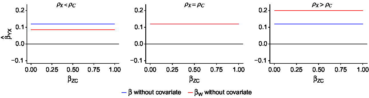
Fig. 2. Results recreated from Frisell et al. (Reference Frisell, Öberg, Kuja-Halkola and Sjölander2012). Blue lines denote the exposure estimate from individual-level models, while red lines denote the exposure estimate from CTC models. The true causal effect is 0 ( ${\beta _{YX}} = 0$
). The within-twin-pair correlations in the exposure and the confounder are
${\beta _{YX}} = 0$
). The within-twin-pair correlations in the exposure and the confounder are ${\rho _X}$
and
${\rho _X}$
and ${\rho _C}$
,
${\rho _C}$
, ${\rm{\;}}$
respectively. For each scenario
${\rm{\;}}$
respectively. For each scenario ${\rho _C}$
= 0.5, while
${\rho _C}$
= 0.5, while ${\rho _X}$
varies between 0.3, 0.5 and 0.7. The bias in the individual-level effect and the within-twin-pair effect does not depend on
${\rho _X}$
varies between 0.3, 0.5 and 0.7. The bias in the individual-level effect and the within-twin-pair effect does not depend on ${\beta _{ZC}}$
, the effect of the confounder on the covariate, because the covariate is not included in these models.
${\beta _{ZC}}$
, the effect of the confounder on the covariate, because the covariate is not included in these models.
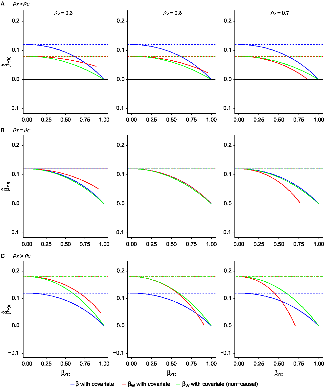
Fig. 3. Exposure effect estimates with the inclusion of a covariate from individual-level and within-pair models when (A) the within-pair correlation in the exposure is less than the within-pair correlation in the confounder; (B) the within-pair correlation in the exposure equals the within-pair correlation in the confounder; (C) the within-pair correlation in the exposure is more than the within-pair correlation in the confounder. For each scenario ${\rho _C}{\rm{\;}}$
= 0.5, while
${\rho _C}{\rm{\;}}$
= 0.5, while ${\rho _X}$
varies between 0.3, 0.5 and 0.7 (consistent with Figure 2). Additionally, each column represents a different value of
${\rho _X}$
varies between 0.3, 0.5 and 0.7 (consistent with Figure 2). Additionally, each column represents a different value of ${\rho _Z}$
, the within-pair correlation in the covariate.
${\rho _Z}$
, the within-pair correlation in the covariate. ${\rm{\;}}{\beta _{ZC}}$
is the effect of the confounder on the covariate. Blue lines denote the exposure estimate from individual-level models, red lines denote the exposure estimate from CTC models as specified in equation 4 and green lines denote the exposure estimate from CTC models as specified in equation 3. Solid lines denote the exposure effect estimate with covariate inclusion, while dashed lines denote the same estimate without covariate inclusion. The true causal exposure effect is 0 (
${\rm{\;}}{\beta _{ZC}}$
is the effect of the confounder on the covariate. Blue lines denote the exposure estimate from individual-level models, red lines denote the exposure estimate from CTC models as specified in equation 4 and green lines denote the exposure estimate from CTC models as specified in equation 3. Solid lines denote the exposure effect estimate with covariate inclusion, while dashed lines denote the same estimate without covariate inclusion. The true causal exposure effect is 0 ( ${\beta _{YX}} = 0$
).
${\beta _{YX}} = 0$
).
Figure 2 shows how nonshared confounding induces bias in both the individual-level and within-pair exposure effect, and how the bias is affected by the relationship between the within-pair correlation in the exposure and the confounder in the absence of covariates (Frisell et al., Reference Frisell, Öberg, Kuja-Halkola and Sjölander2012). The blue line indicates the estimated exposure effect from the individual-level model, while the red line indicates the within-pair effect from the CTC model. Because no covariates are included in either model, bias does not depend on the magnitude of ${\beta _{ZC}}$
. Each panel shows the bias under the possible relationships between
${\beta _{ZC}}$
. Each panel shows the bias under the possible relationships between ${\rho _X}$
and
${\rho _X}$
and ${\rho _C}$
:
${\rho _C}$
: ${\rho _X} \lt {\rho _C}$
,
${\rho _X} \lt {\rho _C}$
, ${\rho _X} = {\rho _C}$
and
${\rho _X} = {\rho _C}$
and ${\rho _X} \gt {\rho _C}$
. As was found in the previous work, when
${\rho _X} \gt {\rho _C}$
. As was found in the previous work, when ${\rho _X} \gt {\rho _C}$
, the βW
estimate from CTC models is a more biased estimate of the exposure effect than the individual-level β.
${\rho _X} \gt {\rho _C}$
, the βW
estimate from CTC models is a more biased estimate of the exposure effect than the individual-level β.
We now consider each relationship between ${\rho _X}$
and
${\rho _X}$
and ${\rho _C}$
separately. Figure 3(A) illustrates the bias when the twin correlation is greater for the covariate than the exposure
${\rho _C}$
separately. Figure 3(A) illustrates the bias when the twin correlation is greater for the covariate than the exposure $\left( {{\rho _C} \gt {\rho _X}} \right)$
with the inclusion of a covariate. In this case, based on findings from Frisell et al. (Reference Frisell, Öberg, Kuja-Halkola and Sjölander2012), we expect that βW
will be less biased than β. We do indeed see that for most values of
$\left( {{\rho _C} \gt {\rho _X}} \right)$
with the inclusion of a covariate. In this case, based on findings from Frisell et al. (Reference Frisell, Öberg, Kuja-Halkola and Sjölander2012), we expect that βW
will be less biased than β. We do indeed see that for most values of ${\rho _Z}$
and
${\rho _Z}$
and ${\beta _{ZC}}$
. As
${\beta _{ZC}}$
. As ${\beta _{ZC}}$
increases, meaning the covariate is an increasingly accurate measure of the confounder, the bias decreases in both βW
and β, as would be expected. The magnitude of
${\beta _{ZC}}$
increases, meaning the covariate is an increasingly accurate measure of the confounder, the bias decreases in both βW
and β, as would be expected. The magnitude of ${\rho _Z}$
, the within-pair correlation in the covariate, affects the rate at which the bias decreases in the βW
coefficients only. When
${\rho _Z}$
, the within-pair correlation in the covariate, affects the rate at which the bias decreases in the βW
coefficients only. When ${\rho _Z}$
is high, the rate of decrease in bias of the βW
estimate is the highest. Comparing both forms of covariate inclusion, when
${\rho _Z}$
is high, the rate of decrease in bias of the βW
estimate is the highest. Comparing both forms of covariate inclusion, when ${\beta _{ZC}}$
is low,
${\beta _{ZC}}$
is low, ${\beta _{{W_{{\rm{cov}}}}}}$
and
${\beta _{{W_{{\rm{cov}}}}}}$
and ${\beta _{{W_{{\rm{covstd}}}}}}$
perform similarly. As the value of
${\beta _{{W_{{\rm{covstd}}}}}}$
perform similarly. As the value of ${\beta _{{\rm{ZC}}}}$
increases,
${\beta _{{\rm{ZC}}}}$
increases, ${\beta _{{W_{{\rm{covstd}}}}}}$
shows less bias at low values of
${\beta _{{W_{{\rm{covstd}}}}}}$
shows less bias at low values of ${\rho _Z},$
while
${\rho _Z},$
while ${\beta _{{W_{{\rm{cov}}}}}}$
shows less bias at high values of
${\beta _{{W_{{\rm{cov}}}}}}$
shows less bias at high values of ${\rho _Z}$
.
${\rho _Z}$
.
Figure 3(B) illustrates the bias with the inclusion of a covariate when ${\rho _X} = {\rho _C}$
. In this case, we expect that βW
will have the same amount of bias as β. This occurs only when
${\rho _X} = {\rho _C}$
. In this case, we expect that βW
will have the same amount of bias as β. This occurs only when ${\rho _Z}$
is also the same (i.e.,
${\rho _Z}$
is also the same (i.e., ${\rho _X} = {\rho _C} = {\rho _Z}$
). When
${\rho _X} = {\rho _C} = {\rho _Z}$
). When ${\rho _Z}$
is low, the within-pair effect is more biased than the individual-level effect. The reverse is true when
${\rho _Z}$
is low, the within-pair effect is more biased than the individual-level effect. The reverse is true when ${\rho _Z}$
is high. As in the previous scenario, as
${\rho _Z}$
is high. As in the previous scenario, as ${\rho _Z}$
increases in magnitude, the rate of bias reduction also increases but only for the within-pair effect. Comparing both forms of covariate inclusion in this scenario,
${\rho _Z}$
increases in magnitude, the rate of bias reduction also increases but only for the within-pair effect. Comparing both forms of covariate inclusion in this scenario, ${\beta _{{W_{{\rm{covstd}}}}}}$
shows similar bias to β across all values of
${\beta _{{W_{{\rm{covstd}}}}}}$
shows similar bias to β across all values of ${\beta _{{\rm{ZC}}}}$
and
${\beta _{{\rm{ZC}}}}$
and ${\rho _Z}$
. As the value of
${\rho _Z}$
. As the value of ${\beta _{{\rm{ZC}}}}$
increases,
${\beta _{{\rm{ZC}}}}$
increases, ${\beta _{{W_{{\rm{cov}}}}}}$
shows increased bias at low values of
${\beta _{{W_{{\rm{cov}}}}}}$
shows increased bias at low values of ${\rho _Z}$
but reduced bias at high values of
${\rho _Z}$
but reduced bias at high values of ${\rho _Z}$
.
${\rho _Z}$
.
Finally, Figure 3(C) illustrates the bias with the inclusion of a covariate when ${\rho _X} \gt {\rho _C}$
. This is the ‘worst case’ scenario where we expect that βW
will have more bias than β. As
${\rho _X} \gt {\rho _C}$
. This is the ‘worst case’ scenario where we expect that βW
will have more bias than β. As ${\beta _{{\rm{ZC}}}}$
increases, the bias in both estimates decreases. Additionally, as
${\beta _{{\rm{ZC}}}}$
increases, the bias in both estimates decreases. Additionally, as ${\rho _Z}$
increases, there comes a point at which βW
is less biased than β. It is clear, however, that this only occurs when
${\rho _Z}$
increases, there comes a point at which βW
is less biased than β. It is clear, however, that this only occurs when ${\rho _Z}$
is high and for narrow ranges of
${\rho _Z}$
is high and for narrow ranges of ${\beta _{{\rm{ZC}}}}$
. Finally, comparing both forms of covariate inclusion, we see a similar relationship between
${\beta _{{\rm{ZC}}}}$
. Finally, comparing both forms of covariate inclusion, we see a similar relationship between ${\beta _{{W_{{\rm{cov}}}}}}$
and
${\beta _{{W_{{\rm{cov}}}}}}$
and ${\beta _{{W_{{\rm{covstd}}}}}}$
as in Figure 3(A). When
${\beta _{{W_{{\rm{covstd}}}}}}$
as in Figure 3(A). When ${\beta _{{\rm{ZC}}}}$
is low,
${\beta _{{\rm{ZC}}}}$
is low, ${\beta _{{W_{{\rm{cov}}}}}}$
and
${\beta _{{W_{{\rm{cov}}}}}}$
and ${\beta _{{W_{{\rm{covstd}}}}}}$
perform similarly. As the value of
${\beta _{{W_{{\rm{covstd}}}}}}$
perform similarly. As the value of ${\beta _{{\rm{ZC}}}}$
increases,
${\beta _{{\rm{ZC}}}}$
increases, ${\beta _{{W_{{\rm{covstd}}}}}}$
shows less bias at low values of
${\beta _{{W_{{\rm{covstd}}}}}}$
shows less bias at low values of ${\rho _Z}$
, while
${\rho _Z}$
, while ${\beta _{{W_{{\rm{cov}}}}}}$
shows less bias at high values of
${\beta _{{W_{{\rm{cov}}}}}}$
shows less bias at high values of ${\rho _Z}$
. Interestingly,
${\rho _Z}$
. Interestingly, ${\beta _{{W_{{\rm{covstd}}}}}}$
never results in less bias than β even at very high values of
${\beta _{{W_{{\rm{covstd}}}}}}$
never results in less bias than β even at very high values of ${\beta _{{\rm{ZC}}}}$
and
${\beta _{{\rm{ZC}}}}$
and ${\rho _Z}$
.
${\rho _Z}$
.
Discussion
The current study extends work by Frisell et al. (Reference Frisell, Öberg, Kuja-Halkola and Sjölander2012) by showing that the inclusion of a covariate as a proxy measure of a confounder always reduces bias in individual-level and CTC exposure effect estimates. However, in situations in which we expect the within-pair estimate (βW ) to me more biased than the individual-level estimate (β), the inclusion of a covariate results in less bias in βW , compared with β, in only a limited set of circumstances. It remains that in most situations likely encountered in practice, βW will be a biased estimate of the true causal exposure effect. This result has important implications for the use and interpretation of CTC, and more broadly between-within, models.
As previously shown in CTC models, when the within-twin-pair correlation in the exposure is greater than the within-pair correlation in the confounder (i.e., ${\rho _X} \gt {\rho _C}$
),
${\rho _X} \gt {\rho _C}$
), ${\beta _W}$
will be more biased than the individual-level β. In this ‘worst case scenario’, one may choose to include a covariate measure as a proxy of the confounder in order to reduce this bias. While covariate inclusion reduces bias in
${\beta _W}$
will be more biased than the individual-level β. In this ‘worst case scenario’, one may choose to include a covariate measure as a proxy of the confounder in order to reduce this bias. While covariate inclusion reduces bias in ${\beta _W}$
more than in β as illustrated in Figure 3, the current work shows that
${\beta _W}$
more than in β as illustrated in Figure 3, the current work shows that ${\beta _W}$
will be less biased than β only when the within-pair correlation in the covariate
${\beta _W}$
will be less biased than β only when the within-pair correlation in the covariate $\left( {{\rho _Z}} \right)$
is high and the covariate is an accurate measure of the confounder (
$\left( {{\rho _Z}} \right)$
is high and the covariate is an accurate measure of the confounder ( ${\beta _{{\rm{ZC}}}}$
is large). In comparing forms of covariate inclusion,
${\beta _{{\rm{ZC}}}}$
is large). In comparing forms of covariate inclusion, ${\beta _{{W_{{\rm{covstd}}}}}}$
generally shows less bias than
${\beta _{{W_{{\rm{covstd}}}}}}$
generally shows less bias than ${\beta _{{W_{{\rm{cov}}}}}}$
when
${\beta _{{W_{{\rm{cov}}}}}}$
when ${\rho _Z}$
is low but shows greater bias at high values of
${\rho _Z}$
is low but shows greater bias at high values of ${\rho _Z}$
. While it may be the case that using
${\rho _Z}$
. While it may be the case that using ${\beta _{{W_{{\rm{covstd}}}}}}$
results in the greatest bias reduction in the exposure effect estimate, this form of covariate inclusion does not retain its assumed causal interpretation (Sjölander et al., Reference Sjölander, Frisell and Öberg2012). The increased bias reduction in select scenarios is not sufficient to justify its use over
${\beta _{{W_{{\rm{covstd}}}}}}$
results in the greatest bias reduction in the exposure effect estimate, this form of covariate inclusion does not retain its assumed causal interpretation (Sjölander et al., Reference Sjölander, Frisell and Öberg2012). The increased bias reduction in select scenarios is not sufficient to justify its use over ${\beta _{{W_{{\rm{cov}}}}}}$
, which does retain the correct causal interpretation.
${\beta _{{W_{{\rm{cov}}}}}}$
, which does retain the correct causal interpretation.
The effect of ${\beta _{{\rm{ZC}}}}$
on these results is intuitive. If the covariate is an accurate measure of the confounder, including it in the model will clearly reduce confounding bias. The effect of
${\beta _{{\rm{ZC}}}}$
on these results is intuitive. If the covariate is an accurate measure of the confounder, including it in the model will clearly reduce confounding bias. The effect of ${\rho _Z}$
on bias reduction is less intuitive. Across all relationships between
${\rho _Z}$
on bias reduction is less intuitive. Across all relationships between ${\rho _X}$
and
${\rho _X}$
and ${\rho _C}$
, increasing values of
${\rho _C}$
, increasing values of ${\rho _Z}$
decrease the bias in the within-pair estimate, as illustrated in Figure 3. In other words, holding
${\rho _Z}$
decrease the bias in the within-pair estimate, as illustrated in Figure 3. In other words, holding ${\rho _X}$
and
${\rho _X}$
and ${\rho _C}$
constant, increasing
${\rho _C}$
constant, increasing ${\rho _Z}$
will reduce bias in βW
(the individual-level estimate, β is not affected by the value of
${\rho _Z}$
will reduce bias in βW
(the individual-level estimate, β is not affected by the value of ${\rho _Z}$
). This occurs for the same reason that increasing
${\rho _Z}$
). This occurs for the same reason that increasing ${\rho _C}$
, holding
${\rho _C}$
, holding ${\rho _X}$
constant, results in lower levels of bias in βW
as discussed in Frisell et al. (Reference Frisell, Öberg, Kuja-Halkola and Sjölander2012). When twins are less discordant on the confounder, meaning that
${\rho _X}$
constant, results in lower levels of bias in βW
as discussed in Frisell et al. (Reference Frisell, Öberg, Kuja-Halkola and Sjölander2012). When twins are less discordant on the confounder, meaning that ${\rho _C}$
is larger, they are also likely to be less discordant on the covariate (
${\rho _C}$
is larger, they are also likely to be less discordant on the covariate ( ${\rho _Z}$
is larger). This decreases the correlation between the covariate and the exposure variables resulting in less bias. Importantly, the within-pair estimate is only unbiased when all confounders are perfectly shared within a twin-pair.
${\rho _Z}$
is larger). This decreases the correlation between the covariate and the exposure variables resulting in less bias. Importantly, the within-pair estimate is only unbiased when all confounders are perfectly shared within a twin-pair.
The current results have important implications for the interpretation of CTC results. As described above, interpretation of the within-pair effect is commonly made by comparing βW
from the CTC model to β from the individual-level model. We show that in the presence of nonshared confounding, CTC results can support a causal effect of exposure on outcome even when the true causal effect is 0 $\left( {{\beta _W} = \beta \ne 0} \right)$
. This will occur even if a covariate is included in the CTC model as a proxy measure of the confounder.
$\left( {{\beta _W} = \beta \ne 0} \right)$
. This will occur even if a covariate is included in the CTC model as a proxy measure of the confounder.
Additionally, the within-pair estimate between the monozygotic $\left( {{\beta _{{W_{{\rm{MZ}}}}}}} \right)$
and dizygotic
$\left( {{\beta _{{W_{{\rm{MZ}}}}}}} \right)$
and dizygotic $\left( {{\beta _{{W_{{\rm{DZ}}}}}}} \right)$
twin-pairs is usually compared to identify whether genetic or shared environmental factors confound the exposure–outcome relationship. For instance, when
$\left( {{\beta _{{W_{{\rm{DZ}}}}}}} \right)$
twin-pairs is usually compared to identify whether genetic or shared environmental factors confound the exposure–outcome relationship. For instance, when ${\beta _{{W_{{\rm{MZ}}}}}} \lt {\beta _{{W_{{\rm{DZ}}}}}} \lt \beta $
, this suggests that the observed relationship is confounded by genetic factors (McGue et al., Reference McGue, Osler and Christensen2010). This is because MZ twin-pairs share all genetic factors, while DZ twin-pairs shared approximately 50% of these factors. Both types of twin-pairs share all common (rearing) environmental factors. Given heritable phenotypes, the within-pair correlation in exposure, confounder and covariate will be greater for MZ compared with DZ twins influencing the comparison of
${\beta _{{W_{{\rm{MZ}}}}}} \lt {\beta _{{W_{{\rm{DZ}}}}}} \lt \beta $
, this suggests that the observed relationship is confounded by genetic factors (McGue et al., Reference McGue, Osler and Christensen2010). This is because MZ twin-pairs share all genetic factors, while DZ twin-pairs shared approximately 50% of these factors. Both types of twin-pairs share all common (rearing) environmental factors. Given heritable phenotypes, the within-pair correlation in exposure, confounder and covariate will be greater for MZ compared with DZ twins influencing the comparison of ${\beta _{{W_{{\rm{MZ}}}}}}$
and
${\beta _{{W_{{\rm{MZ}}}}}}$
and ${\beta _{{W_{{\rm{DZ}}}}}}$
. Even in the case of a true, nonzero effect of exposure on outcome, it would be possible to conclude that genetic factors confound the causal relationship
${\beta _{{W_{{\rm{DZ}}}}}}$
. Even in the case of a true, nonzero effect of exposure on outcome, it would be possible to conclude that genetic factors confound the causal relationship $\left( {{\beta _{{W_{{\rm{MZ}}}}}} \lt {\beta _{{W_{{\rm{DZ}}}}}} \lt \beta } \right)$
when, in reality, they do not. This point has been made previously (Frisell et al., Reference Frisell, Öberg, Kuja-Halkola and Sjölander2012), but we highlight that it continues to hold in the context of the current results.
$\left( {{\beta _{{W_{{\rm{MZ}}}}}} \lt {\beta _{{W_{{\rm{DZ}}}}}} \lt \beta } \right)$
when, in reality, they do not. This point has been made previously (Frisell et al., Reference Frisell, Öberg, Kuja-Halkola and Sjölander2012), but we highlight that it continues to hold in the context of the current results.
Of additional note, it is likely that the exposure and covariate are measured with some amount of error. It is well documented that measurement error in an exposure will attenuate the exposure effect estimate in a simple linear regression (Hutcheon et al., Reference Hutcheon, Chiolero and Hanley2010; Liu, Reference Liu1988; Spearman, Reference Spearman1904). Furthermore, it has been shown that the estimate from CTC models will be attenuated more than individual-level models (Frisell et al., Reference Frisell, Öberg, Kuja-Halkola and Sjölander2012; McGue et al., Reference McGue, Osler and Christensen2010). In the case of multiple regression, where covariates are also subject to measurement error, the estimated exposure effect may under or overestimate the true causal effect (Liu, Reference Liu1988; Rosner et al., Reference Rosner, Spiegelman and Willett1990). While we do not include derivations for β and βW
in the presence of measurement, the reliability of the covariate Z would function as a measure of $\;{\beta _{{\rm{ZC}}}}$
. The effects of measurement error would thus mirror the impact of
$\;{\beta _{{\rm{ZC}}}}$
. The effects of measurement error would thus mirror the impact of ${\beta _{{\rm{ZC}}}}$
as shown in Figure 3.
${\beta _{{\rm{ZC}}}}$
as shown in Figure 3.
While we show that exposure effect estimates from CTC designs are likely to be biased, we maintain that the CTC design can provide useful information when used appropriately. Results from CTC studies can often be used to argue that an observed relationship is not consistent with a causal exposure effect. For instance, when βW
= 0 and the expected level of measurement error does not likely account for this magnitude of attenuation, it would suggest that shared confounders explain at least part of the exposure–outcome relationship. Results may also suggest that an observed association cannot be entirely due to shared confounders within a twin-pair. When ${\beta _W} \ne 0$
, this suggests that some influence beyond shared confounders is contributing to the observed relationship.
${\beta _W} \ne 0$
, this suggests that some influence beyond shared confounders is contributing to the observed relationship.
The best case for bias reduction in CTC model estimates occurs when the within-twin-pair correlation in the exposure is less than the within-twin-pair correlation in the confounder, when the within-twin-pair correlation in the covariate is high, and the covariate is an accurate measure of the confounder. Of these pieces of information, only ${\rho _X}$
and
${\rho _X}$
and ${\rho _Z}$
are known in practice. These values should always be reported and a case should be made about the likely relationships to the possible confounders to determine whether CTC models are appropriate for a given situation. Lastly, there are additional limitations of the CTC design that the current study does not address, like reverse causality and the potential causal influence of nonshared environmental factors not included in the models (McGue et al., Reference McGue, Osler and Christensen2010). Future methodological work should be focused on the extent to which these factors affect exposure effect estimates from CTC models.
${\rho _Z}$
are known in practice. These values should always be reported and a case should be made about the likely relationships to the possible confounders to determine whether CTC models are appropriate for a given situation. Lastly, there are additional limitations of the CTC design that the current study does not address, like reverse causality and the potential causal influence of nonshared environmental factors not included in the models (McGue et al., Reference McGue, Osler and Christensen2010). Future methodological work should be focused on the extent to which these factors affect exposure effect estimates from CTC models.
Supplementary material
To view supplementary material for this article, please visit https://doi.org/10.1017/thg.2019.67
Financial support
This work was supported by grants from the US National Institute on Alcohol Abuse and Alcoholism (R37-AA009367) and the National Institute on Drug Abuse (R01-DA036216).
Conflict of interest
None.


