


Social stratification research involves analyses of the relationships between social background and socioeconomic attainments in education, occupation, and income. Although there are exceptions, the general assumption in the education, sociology, and economic literatures is that these relationships can be attributed wholly to social factors.
However, there is a literature that points out that genetics must be involved in social stratification and socioeconomic attainments (Beenstock, Reference Beenstock2009; Diewald et al., Reference Diewald, Baier, Schulz and Schunck2015; Eckland, Reference Eckland1967; Nielsen, Reference Nielsen2008, Reference Nielsen2016; Scarr & Weinberg, Reference Scarr and Weinberg1978). Theoretical discussions on the relative contributions of genes and environment for socioeconomic outcomes revolve around concepts such as ‘social constraints’ (e.g., Branigan et al., Reference Branigan, McCallum and Freese2013). Where social constraints are considerable, such as severe poverty, poor schooling and discrimination, genetically capable individuals will not reach their full potential (Guo & Stearns, Reference Guo and Stearns2002). In contrast, in contexts where the overwhelming bulk of the population does not face severe social constraints, genetic differences predominate. Over time, social constraints should have been loosened by government legislation, educational expansion, and other societal changes that can be categorized under the rubric of modernization (Colodro-Conde et al., Reference Colodro-Conde, Rijsdijk, Tornero-Gómez, Sánchez-Romera and Ordoñana2015; Heath et al., Reference Heath, Berg, Lindon, Solaas, Corey, Sundet and Nance1985; Le et al., Reference Le, Miller, Slutske and Martin2011; Marks, Reference Marks2014). Nielsen (Reference Nielsen2008) formally relates the relative contributions of genes and the shared environment to modernization and meritocratic theories. Modernization is characterized by high heritabilities and little or no influence from the common environment. In a completely meritocratic society the contribution of the common environment to socioeconomic outcomes would be zero with high heritabilities (Nielsen, Reference Nielsen2008, p. 21).
Twin and kinship studies typically estimate the proportion of variance due to additive genetic effects (A), the common environment (C), and the unique environment that also includes error (E). The same logic applies to contribution of genes to the phenotypical covariation (or correlation) between two traits, referred to as the ‘bivariate heritability’ (Plomin et al., Reference Plomin, DeFries, Knopik and Neiderhiser2013, p. 397). This should not be confused with genetic correlation, which indicates the extent that the same genes are involved in the expression of two different traits (Neale & Maes, Reference Neale and Maes2004, p. 190; Plomin et al., Reference Plomin, DeFries, Knopik and Neiderhiser2013, p. 217).
Although there have been a reasonably large number of ACE studies for educational attainment (see Branigan et al., Reference Branigan, McCallum and Freese2013), there are far fewer studies on occupational status and income. Generally, the heritability of educational attainment in Australia is around 0.50, consistent with an international mean of 0.40 estimated in a recent meta-analysis. The mean estimate for the common environment was 0.35, which is higher than the estimates (C ≈ 0.20) from Australian studies (Branigan et al., Reference Branigan, McCallum and Freese2013). Branigan et al.’s (Reference Branigan, McCallum and Freese2013) meta-analysis of educational attainment showed that, on average, heritability was 0.06 higher among men compared to women and 0.08 higher for those born after 1950 than for those born earlier, and the proportion of the variance attributed to the shared environmental was 0.12 lower for cohorts born after 1950. In contrast, Australian studies show no gender or cohort differences (Baker et al., Reference Baker, Treloar, Reynolds, Heath and Martin1996; Le et al., Reference Le, Miller, Slutske and Martin2011, p. 132; Miller et al., Reference Miller, Mulvey and Martin2001).
For occupational status, heritability estimates tend to be lower than that for education (0.3 to 0.4), with little contribution from the common environment (≈0.10; Behrman et al., Reference Behrman, Hrubec, Taubman and Wales1980, pp. 30–31, 206–207; Fulker, Reference Fulker and Nance1978, p. 231; Tambs et al., Reference Tambs, Sundet, Magnus and Berg1989). Miller et al. (Reference Miller, Mulvey and Martin1996) estimated a heritability of 0.72 for occupational status, considerably higher than estimates from other studies. For Sweden, ACE estimates for occupational status were very different between men (0.60, 0.09, 0.31) and women (0.09, 0.19, 0.72; Lichtenstein et al., Reference Lichtenstein, Pedersen and McClearn1992). For Norway, Tambs et al. (Reference Tambs, Sundet, Magnus and Berg1989) found the heritability of occupational status much higher in younger cohorts compared to the oldest cohort born 1931–1935.
The heritability estimates for income are surprisingly high with moderate or small effects for the common environment and stronger effects for the unique environment. For the United States, Rowe et al.’s (Reference Rowe, Vesterdal and Rodgers1999) ACE estimates were 0.42, 0.23, and 0.35. They concluded that genetics contributed to 25% of the correlation between education and income. Fulker's (Reference Fulker and Nance1978) ACE estimates were 0.47, 0.08, and 0.45, and reported genetic correlations ranging from 0.44 to 0.53 for the genes influencing education, occupational status, and income. In a study of twins and other sibling types in Sweden, Björklund et al. (Reference Björklund, Jäntti, Solon, Bowles, Ginitis and Groves2005) estimated a heritability of 0.28 for male earnings and with negligible effects for the common environment (0.04). The estimates for women were similar. For Sweden, Benjamin et al. (Reference Benjamin, Cesarini, Chabris, Glaeser, Laibson, Gunason and Lichtenstein2012) calculated heritabilities for a single year's income among men and women of 0.37 and 0.28, with no variance attributable to the common family environment. Based on a large number of sibling types, Cesarini's (Reference Cesarini2013, p. 37) heritability estimate for income was lower at 0.27 with negligible effects for the common environment (0.05). For Norway, Ørstavik et al. (Reference Ørstavik, Czajkowski, Roysamb, Knudsen, Tambs and Reichborn-Kjennerud2014) estimated bivariate heritabilities for education and income at 0.37 for men and 0.70 for women, respectively, with large confidence intervals. In a summary of previous studies of genetic and environmental analyses of income, Hyytinen et al. (Reference Hyytinen, Ilmakunnas, Johansson and Toivanen2012) calculated average heritabilities for income (including occupational income) of around 0.40 for Sweden and the United States and 0.45 for Australia. The average proportions of the variance attributable to the common family environment were low: 0.05 for Sweden, 0.09 for the United States, and 0.15 for Australia. Their study of lifetime income in Finland found a much higher income heritability for men (0.58) than women (0.24) but for both sexes ‘the contribution of the shared environment is small or negligible’ (2012, p. 13).
The purpose of this paper was to estimate the contributions of genes, the common environment, and the unique environment to the variances of, and covariances between, educational attainment, occupational status, and income in Australia. Subsequent analyses examine gender and cohort differences. Most previous Australian studies have not directly estimated the ACE variance components but rather only incidentally, because the focus was on the returns to education using the Defries and Fulker (Reference DeFries and Fulker1985) modeling approach. Furthermore, no previous Australian study has used modern statistical procedures to estimate bivariate heritabilities and genetic correlations.
Materials and Methods
Data and Measures
The data were from the 2014 Health and Lifestyle survey based on twins in the Australian Twin Registry (Hopper, Reference Hopper2002). Of the 17,798 twins invited to participate, the online questionnaire was completed by 6,402 respondents, a response rate of 36%. The volunteer sample underrepresents men, comprising only 26% of the sample and with a over representation of monozygotic (MZ) twins (see Table 4). Oversampling of MZ and female twins is common in volunteer twin samples (Lykken et al., Reference Lykken, McGue and Tellegen1987).
Education
In the questionnaire, respondents were asked: ‘What were you and your parents’ highest completed grade level at school?’ The response sets ranged from ‘Did not go to school’ through to ‘Year 8 or equivalent’ to ‘Year 12 or equivalent’. Responses to these questions were used to construct ordinal measures of Years of Education. Vocational qualifications were not included in the construction of the continuous Years of Education measures. Indicative scores were as follows: 8 to 12 for completing that grade level with no post-school university qualifications, 15 for a bachelor degree, and 18 for a master's degree or doctorate.
Occupation
The questionnaire asked respondents their occupation with the following question: ‘If you are working now or have previously worked, what is your usual occupation?’ The text responses were coded to the 4-digit codes in the Australian and New Zealand Occupational Classification schema (Australian Bureau of Statistics, 2006). The 4-digit occupational titles were then recoded to the AUSEI06 measure of occupational status (McMillan et al., Reference McMillan, Beavis and Jones2009). AUSEI06 scales occupations in such a manner as to minimize the direct effect of education on income and maximize the effect of occupational status on income. The AUSEI06 measure ranges from 0 to 100.
Income
The questionnaire asked: ‘What is your current annual income before tax?’ The response categories were as follows: 1 = None; 2 = $1–$15,600; 3 = $15,601–$31,200; 4 = $31,200–$52,000; 5 = $52,001–$78,000; 6 = $78,001–$104,000; 7 = $104,001–$126,000. Here, income includes job earnings, investments, and government benefits. Incomes were recoded to the midpoints of each category. For the highest category, the income assigned ($150,000) was calculated using the Pareto distribution (Parker & Fenwick, Reference Parker and Fenwick1983). Zero incomes were reassigned an annual income of one dollar. The continuous distribution approximated a normal distribution, although there was an excess of respondents with zero income. The skewness and kurtosis statistics were 0.4 and 0.7, respectively.
Table 1 presents univariate statistics for the variables used in these analyses. The average number of years of education is nearly 14 years, the average occupational status is 65, and the average income $60,000 per annum. For the statistical analyses, the measures of occupational status and income were divided by 10 and 10,000, respectively, and the three outcome measures were centered about their means. These data transformations facilitate estimation of the coefficients.
TABLE 1 Univariate Statistics for Analysis Variables

Table 2 presents the means and standard deviations of the outcome variables, which are very similar for the MZ and dizygotic (DZ) twin groups. Table 3 presents the correlations for the main variables used in these analyses. The correlations of the AUSEI06 measure of occupational status with education and income are consistent with other Australia data (Broom et al., Reference Broom, Jones, McDonald and Williams1980, p. 26; McMillan et al., Reference McMillan, Beavis and Jones2009). The simple test described by Jinks and Fulker (Reference Jinks and Fulker1970) for gene-environment interactions by correlating the sum and absolute differences for the response variable among MZ twins showed very weak and non-significant correlations (−0.03 < r < 0.03) for all three outcomes. Therefore, there was no need to further transform the scales of measurement to remove gene-environment interactions.
TABLE 2 Mean and Standard Deviations for Analysis Variables by Zygosity

Zygosity was unknown for 32 respondents.
TABLE 3 Correlations for Variables

M = male, F = female.
Table 4 presents the within-twin pair correlations for educational attainment, occupational status, and income. The first panel presents the data and correlations for all twins, the second panel by zygosity, the third by gender and zygosity, and the bottom panel by broad cohort and zygosity. These groups form the data for the analyses presented later. Note that the numbers of twin pairs in each group are much less than the numbers of individual twins, but data from non-paired twins was utilized in the analyses (see below).
TABLE 4 Correlations for Twin Groups

Statistical Methods
The estimates presented in this article were obtained using the OpenMX software package (Boker et al., Reference Boker, Neale, Maes, Wilde, Spiegel, Brick and Fox2011; Neale et al., Reference Neale, Hunter, Pritikin, Zahery, Brick, Kirkpatrick and Boker2016; OpenMx Development Team, 2014). The logic of the program is to define the path coefficients for a, c, and e and for the path equations for the covariates (sex and age), subset the data for into the various twin groups, define the model-implied expected covariances and means, and combine the separate models for each group. The models include adjustments for age and gender using regression equations since there are age and gender effects on these outcomes; without these adjustments, the twin correlations are over-estimated (McGue & Bouchard Jr., Reference McGue and Bouchard1984).
The coefficients were estimated using full information maximum likelihood (FIML), which compares the observed data and predicted means and covariances for each row of twin-pair data rather than the sample and predicted variance-covariance matrices. OpenMx allows the estimation of likelihood-based confidence intervals for each parameter estimated (Neale et al., Reference Neale, Hunter, Pritikin, Zahery, Brick, Kirkpatrick and Boker2016; Neale & Miller, Reference Neale and Miller1997). They are the lowest and highest parameter estimates at which there is a statistically significant deterioration in model fit.
Missing values were handled as follows. If one twin was missing on age, the missing value was replaced by the age of the cotwin, if not missing. This procedure was also used for gender among MZ but not DZ twins. For the three analysis variables, FIML handles missing data by filtering out missing values when they are present and using only the data that are not missing in a given row of data (Boker et al., Reference Boker, Neale, Maes, Wilde, Spiegel, Brick and Fox2011, pp. 166–167). FIML is generally superior to multiple imputation for missing data with minor violations from multivariate normal distributions (Yuan et al., Reference Yuan, Yang-Wallentin and Bentler2012). So, cases deleted were twin pairs with no data on zygosity; no age data for both twins; DZ twin pairs with missing data on gender for either twin; or twin pairs missing on all six analysis variables. With these case-wise deletions, the total number of twin pair observations analyzed was 3086. Baraldi and Enders (Reference Baraldi and Enders2010) provide an accessible introduction to maximum likelihood estimation and how FIML handles missing data.
The multivariate analysis is based on the trivariate Cholesky model. In the initial saturated Cholesky model, there are latent genetic and environmental sources corresponding to three outcomes: education, occupation, and income (see Figure 1). Subsequently, more parsimonious models are tested by removing some statistically insignificant coefficients until no coefficient was statistically insignificant. For competing models with the same number of significant coefficients, the likelihood ratio and Akaike's Information Criterion (AIC) were used for model selection (Neale & Maes, Reference Neale and Maes2004, p. 163).

FIGURE 1 Full three-variable Cholesky model.
Results and Discussion
Table 5 presents the characteristics and fit statistics for the various models tested. Model 1 is the initial full Cholesky model for all twin pairs with all parameters (a11, a21, a31 . . .) free. Comparison of model 2 with model 1 shows that all the common family parameters can be deleted from the model without a statistically significant increase in the likelihood ratio. In contrast, removal of the genetic factors significantly increases the likelihood ratio (model 3 vs. model 1). Model 4 is the preferred model since it has five fewer estimated parameters without a statistically significant deterioration in model fit, includes statistically significant common family parameters, and exhibits the lowest AIC value. This is the preferred model from the substantial number of models investigated. In this and subsequent models, there is only one latent common environmental factor, so there are no specific latent common environmental factors for education, occupation, and income. Therefore, correlations of the common environmental influences across outcomes (corresponding to the genetic correlations) are not applicable.
TABLE 5 Summary Fit Measures for Modified Cholesky Models of Education, Occupation, and Income

Preferred models in bold type. The number of twin pair observations for each model is 3,086. f = female, m = male, y = younger, o = older.
Model 4 was used as the basis to investigate gender (models 5 and 6) and cohort (models 7 and 8) differences. Comparisons of the likelihood ratios for models 5 and 7 with that of model 4 show that separate parameters for gender and cohorts significantly improves model fit and reduces the AIC statistic. Therefore, there are gender and cohort differences in the parameter estimates. Analysis of model 5 revealed that the coefficient a31 was not statistical significant for men, but was highly significant for women. Deleting this element from the gender model (fixing its value at zero for men) did not significantly worsen the fit and reduced the AIC statistic. Similarly, analysis of model 7 revealed that the coefficient c11 was not statistically significant for the older cohort and its deletion from the older cohort model improved the model statistics.
Figure 2 presents the standardized path coefficients for the preferred model. In the full Cholesky model, all the confidence intervals for parameters a31, a22, a32, and a33, and all the common environment parameters, include zero. In contrast to the full Cholesky, in the preferred model none of the confidence intervals include zero and the confidence intervals for the estimates for a11 and a21 are narrower.

FIGURE 2 Estimated standardized path coefficients for preferred Cholesky model (model 4).
Table 6 presents the standardized variance/covariance estimates from the preferred model. The leading diagonals are the estimates of heritability estimates and confidence intervals [95% CI]. For the preferred model, the heritabilities are 0.54 [0.44, 0.60] for educational attainment, 0.37 [0.32, 0.42] for occupational status, and 0.18 [0.09, 0.35] for income. The heritability estimates for education and occupation are consistent with previous studies with the heritability for education over 0.5 and lower for occupation. However, the heritability estimate for income is lower than that obtained from most previous studies, although the estimate is not too dissimilar from that of Cesarini (Reference Cesarini2013) and Björklund et al. (Reference Björklund, Jäntti, Solon, Bowles, Ginitis and Groves2005) for Sweden. The low heritability for income found in this study is not because the measure analyzed is income rather than job earnings since limiting income to those working did not increase the heritability estimate. One explanation is that in this study income was measured across the entire age distribution, whereas in most previous studies income was measured among only younger cohorts. For older persons, there is more time for unique environmental factors to come into play that reduce the similarity of incomes among twins: differential job and thus income histories, differences in labor market participation associated with marital status, children and life-course stage, and retirement incomes that largely reflect pre-retirement labor force participation and incomes. Technical factors such as the categorical measure, inaccuracies in reporting, and the presence of zero incomes are probably not responsible for the lower heritability since these factors are not likely to affect MZ twin pairs more than DZ twin pairs.
TABLE 6 Proportions of Phenotype Variances and Covariances Due to Genes, the Common Environment, and Unique Factors (Model 4)
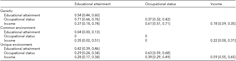
Diagonal entries are proportions of the variance. Off-diagonal entries are proportions of the covariance. 95% confidence intervals are in parentheses.
The estimates for the contribution of the common environment are 0.04 [0.00, 0.13] for education and occupation (set at zero), which are generally less than the estimates reported in the literature. This may be because respondents in this study were born later than respondents in previous studies. In contrast, the common environment estimate for income at 0.22 [0.08, 0.31] is higher than most estimates in the literature.
The off-diagonal elements in Table 6 are the proportions of the covariance (correlations) attributed to each of the three components. The preferred model estimates bivariate heritabilities of about 0.7 for education and occupation, 0.4 for education and income, and 0.6 for occupation and income. The estimate for the bivariate heritability of education and income is associated with wide confidence intervals 0.37 [0.18, 0.74], due to gender differences (see below). The proportions of the covariances due to unique environmental factors were 0.3 for education with both occupation and income and 0.4 for occupation and income.
Table 7 presents the standardized ACE estimates obtained from the gender analysis. The heritability of educational attainment is only marginally higher among women than men, confirming the general conclusion from the Australian literature of no gender differences in the heritability of education. The gender differences in income were contrary to expectations. The heritability of income among women (0.22) is about twice that among men (0.11), and the common environment estimate is substantially larger among men (0.36) than women (0.16). There is no clear explanation for these findings. The other notable gender difference is that the bivariate heritability for education and income is 0.44 for women but zero for men. Correspondingly, the extent that the common environment accounts for the covariation between education and income is substantially higher among men (0.69) than women (0.29). This is the opposite finding to that of Ørstavik et al. (Reference Ørstavik, Czajkowski, Roysamb, Knudsen, Tambs and Reichborn-Kjennerud2014) that found higher bivariate heritabilities for education and income among women.
TABLE 7 Proportions of Phenotype Variance–Covariance Due to Genes, the Common Environment, and Unique Factors by Gender (Model 6)

95% confidence intervals are in parentheses.
Table 8 presents the ACE estimates obtained from the cohort analysis. There are no significant cohort differences in the heritabilities of educational attainment and occupational status. Although the heritability of income is low in both cohorts, it is significantly higher in the older cohort compared to the younger cohort. Correspondingly, the contribution of the common environment is twice as large in the younger cohort. These findings run counter to the expectations of modernization theory. The only finding that weakly supports modernization theory is the absence of a contribution from the common environment on education in the younger cohort whereas there is a significant, albeit small, contribution for the older cohort. Similarly, the contribution of the common environment to the covariance between education and income was estimated at 0.42 in the older cohort but zero in the younger cohort. Therefore, it can be concluded that for education, the common environment has no impact on the variation in education for the younger cohort, although there are no cohort differences in its heritability.
TABLE 8 Proportions of Phenotype Variance–Covariance Due to Genes, the Common Environment, and Unique Factors by Cohort (Model 8)

95% confidence intervals are in parentheses.
The genetic and environmental correlations are presented in Table 9. There is a high correlation in the genes that influence education and occupation (0.8> r > 0. 9), a much weaker genetic correlation between genes that influence education and income (r ≈ 0.4), and a sizable genetic correlation between occupation and income (r ≈ 0.75). Among men, the best estimate for the genetic correlation between education and income is zero. The point estimates for the genetic correlations with income are substantially larger in the younger cohort but the associated confidence intervals are very large and overlap so that the conclusion is no significant difference. The correlations for the unique environment are weaker than the genetic correlations: 0.3 for the unique environmental factors that affect both education and occupation, 0.15 for the unique environmental factors that affect both education and income, and 0.2 for the unique environmental factors that affect both occupation and income.
TABLE 9 Genetic and Environmental Correlations

The common environmental correlations in the full Cholesky model were associated with confidence intervals ranging from −1 to 1. In all other models only one common latent environment factor was specified so rC correlations are not relevant.
Conclusions
In their analysis of the heritability of educational attainment, Lucchini et al. (Reference Lucchini, Della Bella and Pisati2013) conclude that traditional sociological theories used to explain individual differences in educational achievement may not be ‘the best ones’, and that it is crucial to consider both genetic as well as environmental influences. This study reiterates that conclusion for education in Australia and extends it to occupation and income and the relationships between these three outcomes. Few studies of occupational attainment, the socioeconomic career, and income very rarely consider that genetics are involved. Social science theories on social stratification fail if they do not acknowledge that genes are involved in people's socioeconomic attainments.
These studies provide some support for modernization theory. For education and occupation, the contributions of the shared environment were negligible. These findings indicate that the processes involved in educational and occupational attainment in Australia are largely meritocratic. However, for none of three outcomes were the heritabilities substantially higher in the younger cohort compared to the older cohort. One explanation for the lack of cohort differences as hypothesized by modernization theory is that the processes of modernization that reduced the importance of the common environment in Australia occurred decades ago so would not be apparent in comparisons of cohorts in data collected recently.
Conflict of Interest
None.
Ethical Standards
All procedures performed in studies involving human participants were in accordance with the ethical standards of the institutional and/or national research committee and with the 1964 Helsinki declaration and its later amendments or comparable ethical standards. The project has been approved by the Australian Catholic University Ethics committee (Ethics Register Number: 2015–203N). Project title: Genetic and Environment Components to the Educational and Socioeconomic Attainments of Australians. Informed consent was obtained from all individual participants included in the study. Participation in the study was voluntary.


