


1. Introduction
The demand to improve health quality has led to much research including, phonomicrosurgeries, which involves delicate surgical operations on the vocal fold and requires a highly skilled surgeon [Reference Zeitels1, Reference Giallo, Lalush, Nagle, Finley, Buckmire and Grant2]. Vocal fold surgery requires precision and accuracy due to the tissue’s nature being resected, thin, fragile, and viscous. Their lesions might be less than 1 mm [Reference Eckel, Berendes, Damm, Klussmann and Wassermann3, Reference Remacle4]. The most common procedure to resect those lesions relies on laser surgery.
Systems for laser phonosurgery, such as Acupulse Duo by Lumenis [Reference Israel5], are based on a laser manipulator mounted onto an external microscope. The patient is placed in extreme neck extension so that a rigid straight laryngoscope can be placed in the patient mouth and throat to allow a direct line of sight between the laser manipulator and vocal fold in the larynx. However, certain vocal fold portions are inaccessible in such a placement as lateral and posterior sides because the laser source is located out of the patient’s body. A small area laser beam could be moved into the laryngoscope, which prevents the surgeon from conducting a surgical operation on those portions.
Another system, a flexible endoluminal robotic system, was developed during the European project µRALP [Reference Mattos and Andreff6]. That concept has a miniaturized laser manipulator, having micro cameras embedded at the endoscope tip and shooting laser from within the larynx. Nevertheless, since the laser source was placed above the vocal fold and light only travels along straight lines hindered the surgeon from operating on the anterior vocal fold but hardly had access to lateral sides and, to the best of our knowledge, no access to the posterior side. The µRALP project also proposed improving laser steering accuracy by automatically controlling the laser [Reference Renevier, Tamadazte, Rabenorosoa, Tavernier and Andreff7] to follow a surgeon-drawn path [Reference Mattos, Deshpande, Barresi, Guastini and Peretti8], rather than having the surgeon manually steer the laser beam through a poorly ergonomic joystick. This automatic control is done by visually servoing laser spots from one [Reference Renevier, Tamadazte, Rabenorosoa, Tavernier and Andreff7] or two [Reference Andreff and Tamadazte9, Reference Tamadazte and Andreff10] endoscopic cameras.
There are several works reported in the literature, especially in visually guided laser ablation catheter [Reference Dukkipati, Kuck, Neuzil, Woollett, Kautzner, McElderry, Schmidt, Gerstenfeld, Doshi, Horton, Metzner, d’Avila, Ruskin, Natale and Reddy11], which was designed to allow the operator to directly visualize target tissue for ablation and then deliver laser energy to perform point-to-point circumferential ablation. Also, the velocity independent visual path following for laser surgery in ref. [Reference Seon, Tamadazte and Andreff12] where nonholonomic control of the unicycle model and path following at high frequency to satisfy the constraints of laser–tissue interaction was explored. Another example is reported in ref. [Reference Muddassir, Gomez, Hu, Chen and Navarro-Alarcon13], where a robotic system for skin photo-rejuvenation, which uniformly delivers laser thermal stimulation to a subject’s facial skin tissue, was investigated. Yet, as far as we could understand it, none of those work automatically steered laser along hidden paths.
Visual servoing techniques use visual information extracted from the images to design a control law [Reference Espiau, Chaumette and Rives14–Reference Sanderson and Weiss16]. It is a systematic way to control a robot using the information provided by one or multiple cameras [Reference Chaumette and Hutchinson17]. Standard stereo sensors used for visual servoing have a limited view and consequently limit their application range. Hence, using planar mirrors has been prioritized to enlarge the field of view of classic pinhole cameras [Reference Mariottini, Scheggi, Morbidi and Prattichizzo18] and for high-speed gaze control [Reference Iida and Oku19, Reference Okumura, Oku and Ishikawa20]. A planar mirror is a mirror with a planar reflective surface. An image of an object in front of it appears to be behind the mirror plane. This image is equivalent to one being captured by a virtual camera located behind the mirror; additionally, the virtual camera’s position is symmetric to the position of the real camera. In our case, the camera’s reflection in the planar mirror is used to track virtual features points in the vocal fold hidden scene. For instance, by using mirror reflections of a scene, stereo images are captured [Reference Mariottini, Scheggi, Morbidi and Prattichizzo21].
Tracking is the problem of estimating the trajectory of an object in the image plane as it moves around a scene. A tracker allocates unswerving labels to the tracked objects in different video frames. In addition, depending on the tracking field, a tracker can provide object-centric information, such as the area or shape of an object. Simple algorithms for video tracking rely on selecting the region of interest in the first frame associated with the moving objects. Tracking algorithms can be classified into three categories: point tracking [Reference Rasmussen and Hager22, Reference Hue, Le Cadre and Pérez23], kernel tracking [Reference Zhou, Chellappa and Moghaddam24, Reference Nguyen and Smeulders25], and silhouette tracking [Reference Yilmaz, Li and Shah26]. Occlusion can significantly undermine the performance of the object tracking algorithms. Occlusion often occurs when two or more objects come too close and seemingly merge or combine. Image processing systems with object tracking often wrongly track the occluded objects [Reference Zhao, Tian, Zhang and Wei27]. After occlusion, the system will wrongly identify the initially tracked objects as new objects [Reference Shehzad, Shah, Mehmood, Malik and Azmat28]. If the geometry and placement of static objects in the real surroundings are known, the so-called phantom model is a common approach for handling the occlusion of virtual objects. A method for detecting a dynamic occlusion in front of static backgrounds is described in ref. [Reference Fischer, Regenbrecht and Baratoff29]. This algorithm does not require any previous knowledge about the occluding objects but relies on a textured graphical model of planar elements in the scene. Some approaches solve the occlusion problem using depth information delivered by stereo matching [Reference Wloka and Anderson30]. In our approach to the occlusion problem, we use the triangulation method, where we pay attention to the pixels which are well reconstructed when an image is reproduced and ignore the ones which are not well reconstructed.
The study focussed on a conceptual method of servoing laser to hidden parts of the vocal fold. Having been inspired by this clinical need for improved access and those work pieces on mirror reflections, we propose an analysis of anatomical constraints of the vocal fold, devised a conceptual design, and formulated a controller, which was evaluated experimentally on a tabletop setup.
The first contribution is to propose a method to access parts of the vocal fold workspace that are not directly visible during phonomicrosurgery, for instance, the posterior side of the vocal fold by seeing through an auxiliary mirror to overpass the limited micro-cameras field of view of a flexible endoscopy system that was missing in ref. [Reference Renevier, Tamadazte, Rabenorosoa, Tavernier and Andreff7], and shooting surgical laser using the same auxiliary mirror to access those invisible parts in the vocal fold workspace. The second contribution is to derive the control equations for automatically steering the laser through the auxiliary mirror to the hidden parts of the vocal fold by updating the control in refs. [Reference Andreff and Tamadazte9, Reference Tamadazte and Andreff10]. However, through modelling, simulation, and experimentation, the addition of the auxiliary mirror is shown to have no impact, which is thereby demonstrated as being used as it is. Nonetheless, we took the opportunity of this study to derive a variant of the control in ref. [Reference Andreff and Tamadazte9] based on the geodesic error (cross-product) rather than on the linear error. Fig. 1 shows a sample of a simulated image of the vocal fold.

Figure 1. Simulated image of vocal fold anatomy.
The remainder of this study is presented as follows. Section 2 gives a detailed description of the conceptual system design to access parts of the vocal fold. Section 3 deals with modelling the proposed system both in monocular and stereoscopic cases to establish a controller. Section 4 focuses on the simulation results of the controller for both the monocular case and stereoscopic case. Section 5 presents the performed experimental validations in a tabletop setup.
2. Design
2.1. System configuration
As illustrated in Fig. 2, the objective is to devise a method that improves access to hidden parts of the vocal fold. In our approach, we propose a system with two cameras to give stereo view and visual feedback to the scene, a laser source to provide surgical laser needed for tissue ablation, illumination guidance, auxiliary mirror guide, and an auxiliary mirror manipulator through which laser is steered to hidden parts of the vocal fold. In practice, human tissues will never contact the designed micro-robotic device, just the endoscope outer shell, which can be readily sterilized and biocompatible. An auxiliary mirror would be inserted at the beginning of the surgical process and remain stationary until the end of surgery. All those parts must be miniaturized and enclosed in a flexible endoscope during fabrication which is out of this paper’s scope. However, details on packing all those hardware components (miniaturized) into an endoscope can be found in ref. [Reference Tamadazte, Renevier, Séon, Kudryavtsev and Andreff31]

Figure 2. System configuration.
2.2. System model for accessing hidden parts of vocal fold
From the system configuration above, enlarging its distal arrangements of a flexible endoscope and focussing on how to access hidden features of the vocal fold is shown in Fig. 3. The system has a micro-robot, a tip/tilt actuating mirror to steer the laser through an auxiliary mirror to reach hidden parts. The two cameras also observe the same hidden scene through a mirror reflection. Hence, providing a clear vision of the surgeon’s stage to define a trajectory followed automatically by surgical laser in those hidden parts.

Figure 3. System model.
2.3. Enlarged anterior, lateral, and posterior view for accessing hidden parts of vocal fold
The former configuration of Fig. 2 has a limited field of view, even on anterior parts of the vocal fold, because of technical constraints (miniaturization for endoluminal systems, direct line of sight for extracorporeal systems). Thus, the proposed method for accessing hidden parts on the vocal fold anterior side is in Fig. 4(a). Based on the orientation and position of the auxiliary mirror, the surgical laser can be steered to all parts on the anterior side of the vocal fold, which is the surface of the vocal fold that is visible from the larynx. For instance, the laser can reach parts outside of the direct view field (in yellow).

Figure 4. (a) Anterior view access. (b) Lateral view access. (c) Posterior view access.
Table I. List of symbols used in the paper.

In Fig. 4(b), a surgical laser is first shot to an auxiliary mirror, then reflected towards the tissues located above the vocal fold in the larynx, such as the ventricular fold.
As demonstrated in Fig. 4(c), rare portions of a vocal fold being the surface visible from the trachea can be accessed by opening the vocal lips using forceps, exposing the backside for the auxiliary mirror to be oriented and pushed.
3. Modelling
3.1. Mirror reflection
From a technical point of view, these control equations also differ from the already published ones [Reference Renevier, Tamadazte, Rabenorosoa, Tavernier and Andreff7, Reference Andreff and Tamadazte9, Reference Tamadazte and Andreff10] by the use of an alternative formulation of the perspective projection model and by the servoing of geodesic image errors instead of linear image errors. Table I shows list of symbols used in the paper.
Consider the reflection of $\boldsymbol{{X}}$
into
$\boldsymbol{{X}}$
into $\boldsymbol{{X}}_{R}$
through the auxiliary mirror plane
$\boldsymbol{{X}}_{R}$
through the auxiliary mirror plane $\pi = (\underline{\boldsymbol{n}}^T, d )^T$
where
$\pi = (\underline{\boldsymbol{n}}^T, d )^T$
where $\underline{\boldsymbol{n}}$
is the vector normal to the mirror plane, and d is the distance of the reference frame origin to the mirror plane. Using homogeneous coordinates for the points and following [Reference Marchand and Chaumette32], one has
$\underline{\boldsymbol{n}}$
is the vector normal to the mirror plane, and d is the distance of the reference frame origin to the mirror plane. Using homogeneous coordinates for the points and following [Reference Marchand and Chaumette32], one has
 \begin{align}\tilde{\boldsymbol{X}}_{R} = \mathrm{D} \tilde{\boldsymbol{X}}\end{align}
where
 \begin{align} \mathbf{D}= \begin{bmatrix} \mathbf{I} - {2}\underline{\boldsymbol{n}}\underline{\boldsymbol{n}}^T & \quad {2}{d}\underline{\boldsymbol{n}}\\[5pt] \boldsymbol{0}_{\boldsymbol{3 \times 1}}^T & \quad 1 \end{bmatrix}\end{align}
Implementing these equations depends on the chosen reference frame and can thus be expressed either in the world frame.
 \begin{align}{}^w\tilde{\boldsymbol{X}}_{R} = {}^{{w}}\mathrm{D}{}^w\tilde{\boldsymbol{X}}\end{align}
or in a camera frame
 \begin{align}{}^c\tilde{\boldsymbol{X}}_{R} = {}^{{c}}\mathrm{D}{}^c\tilde{\boldsymbol{X}}\end{align}
3.2. Camera projection based on a cross-product concept
When a camera captures an image of a scene, depth information is lost as objects, and points in 3D space are mapped onto a 2D image plane. For the work in this study, depth information is crucial since there is a need for scene reconstruction from the information provided by the 2D image to know the distance between the actuated mirror and the scene without prior knowledge of where they are. Therefore, the used approach of the perspective (pinhole) image projection $\boldsymbol{{x}}$
of a 3D point
$\boldsymbol{{x}}$
of a 3D point $\boldsymbol{{X}}$
is stated as
$\boldsymbol{{X}}$
is stated as
 \begin{align} {}^{im}\tilde{\boldsymbol{x}} \equiv{} {}^{im}\tilde{\mathbf{K}}_{c} \mathbf{I}_{3\times4} {}^{c}{\textbf{T}}_w {}^{{w}}\mathbf{D} {}^{w}\tilde{\boldsymbol{X}}\end{align}
where ${}^{im}\tilde{\mathbf{K}}_c$
represents calibrated intrinsic camera parameters,
${}^{im}\tilde{\mathbf{K}}_c$
represents calibrated intrinsic camera parameters, $\mathbf{I}_{3\times4}$
represents a canonical perspective projection in the form of
$\mathbf{I}_{3\times4}$
represents a canonical perspective projection in the form of $\boldsymbol{3} \times \boldsymbol{4}$
identity matrix,
$\boldsymbol{3} \times \boldsymbol{4}$
identity matrix, ${}^{c}{\textbf{T}}_w$
represents Euclidean 3D transformation (rotation and translation) between the two coordinate systems of camera and world through a mirror. The
${}^{c}{\textbf{T}}_w$
represents Euclidean 3D transformation (rotation and translation) between the two coordinate systems of camera and world through a mirror. The $\equiv{}$
sign represents depth loss in the projection up to some scale factor. In practice, the
$\equiv{}$
sign represents depth loss in the projection up to some scale factor. In practice, the $ \equiv{}$
sign can be removed through division operation, which introduces non-linearity. Alternately, using the cross product, we can make the projection equation a linear constraint equation. Since the light ray emitted from the camera centre point aligns with the light ray coming from the 3D point. If we treat light ray emitted from the camera centre point as vector
$ \equiv{}$
sign can be removed through division operation, which introduces non-linearity. Alternately, using the cross product, we can make the projection equation a linear constraint equation. Since the light ray emitted from the camera centre point aligns with the light ray coming from the 3D point. If we treat light ray emitted from the camera centre point as vector $\boldsymbol{{A}}$
and light ray coming from the 3D point as vector
$\boldsymbol{{A}}$
and light ray coming from the 3D point as vector $\boldsymbol{{B}}$
. The cross-product of two 3D vectors
$\boldsymbol{{B}}$
. The cross-product of two 3D vectors $\boldsymbol{{A}}$
and
$\boldsymbol{{A}}$
and $\boldsymbol{{B}}$
gives another vector with a magnitude equal to that of the area enclosed by the parallelogram formed between the two vectors. The direction of this vector is perpendicular to the plane enclosed by
$\boldsymbol{{B}}$
gives another vector with a magnitude equal to that of the area enclosed by the parallelogram formed between the two vectors. The direction of this vector is perpendicular to the plane enclosed by $\boldsymbol{{A}}$
and
$\boldsymbol{{A}}$
and $\boldsymbol{{B}}$
in the direction given by the right-hand rule, and the magnitude of the cross product will be given by
$\boldsymbol{{B}}$
in the direction given by the right-hand rule, and the magnitude of the cross product will be given by $\mid \boldsymbol{{A}} \mid \mid \boldsymbol{{B}} \mid \sin\theta$
. However, if these two vectors are in the same direction, just like in our case, the angle between them will be zero. The magnitude of the cross product will be zero since
$\mid \boldsymbol{{A}} \mid \mid \boldsymbol{{B}} \mid \sin\theta$
. However, if these two vectors are in the same direction, just like in our case, the angle between them will be zero. The magnitude of the cross product will be zero since $\sin(0) = 0$
. The resultant vector will be the zero vector.
$\sin(0) = 0$
. The resultant vector will be the zero vector. $ \boldsymbol{{A}} \times \boldsymbol{{B}} = 0$
 \begin{align}\begin{bmatrix} {}^{im}\tilde{\mathbf{K}}_c^{-1}{}^{im}\tilde{\boldsymbol{x}} \end{bmatrix}_\times { \mathbf{I}_{3\times4} {}^{c}{\textbf{T}}_w {}^{{w}}\mathbf{D}}{}^{w}\tilde{\boldsymbol{X}} = \boldsymbol{0}\end{align}
Hence for notation simplicity, let
 \begin{align} {}^c\tilde{x} = {}^{im}\tilde{\mathbf{K}}_c^{-1}{}^{im}\tilde{\boldsymbol{x}}\end{align}
 \begin{align} {}^{c}{\boldsymbol{G}}_w = { \mathbf{I}_{3\times4} {}^{c}{\textbf{T}}_w {}^{{w}}\mathbf{D}}\end{align}
Consequently, Eq. (6) rewrites more simply as
 \begin{align}[ {}^c\tilde{\boldsymbol{x}}]_\times {}^{c}\mathbf{G}_w{}^w\tilde{\boldsymbol{X}} = 0\end{align}
3.3. Laser spot kinematics
The time derivative of Eq. (9) is considered to servo the spot position from the current position to the desired one while the camera and mirror remain stationary.
 \begin{align} [ {}^c\dot{\tilde{\boldsymbol{x}}}]_\times {}^{c}\mathbf{G}_w{}^w\tilde{\boldsymbol{X}} + [ {}^c\tilde{\boldsymbol{x}}]_\times {}^{c}\mathbf{G}_w{}^w\dot{\tilde{\boldsymbol{X}} } = \boldsymbol{0} \end{align}
Since ${}^c\tilde{\boldsymbol{x}}$
is a unit vector (i.e.
${}^c\tilde{\boldsymbol{x}}$
is a unit vector (i.e. $\|{}^c\tilde{\boldsymbol{x}}\| = \boldsymbol{1}$
) and using Eq. (9) yields
$\|{}^c\tilde{\boldsymbol{x}}\| = \boldsymbol{1}$
) and using Eq. (9) yields
 \begin{align}^{c}\mathbf{G}_w{}{}^w\tilde{\boldsymbol{X}} = \delta_c {}^c\tilde{\boldsymbol{x}}\end{align}
with $ \delta_c > 0$
the unknown depth along the line of sight passing through
$ \delta_c > 0$
the unknown depth along the line of sight passing through $ {}^c\tilde{\boldsymbol{x}}$
hence, Eq. (10) becomes
$ {}^c\tilde{\boldsymbol{x}}$
hence, Eq. (10) becomes
 \begin{align} [ {}^c\tilde{\boldsymbol{x}}]_\times {}^c\dot{\tilde{\boldsymbol{x}}} = \dfrac{1}{\delta_c {}}[ {}^c\tilde{\boldsymbol{x}}]_\times {}^{c}\mathbf{G}_w{}^w\dot{\tilde{\boldsymbol{X}}}\end{align}
3.4. Scanning laser mirror as a virtual camera
Scanning a mirror as a virtual camera is considered with a virtual image plane. Therefore, the mathematical relationship between it and the 3D spot on the reflected vocal fold is established in Eq. (13) below. Some parameters of Eq. (6) have changed as $c = m$
, and
$c = m$
, and $\mathbf{K}=\mathbf{I}_{3\times3}$
since when using the mirror as a camera, focal length, optical centre, and lens distortion are no longer a problem hence
$\mathbf{K}=\mathbf{I}_{3\times3}$
since when using the mirror as a camera, focal length, optical centre, and lens distortion are no longer a problem hence $\mathbf{K}$
is taken to be one.
$\mathbf{K}$
is taken to be one.
 \begin{align} [{}^{m}z]_\times\mathbf{I}_{3\times4} {}^{m}\mathbf{T}_w{}{}^{{w}}\mathbf{D} {}^w\tilde{\boldsymbol{X}} = \boldsymbol{0}\end{align} ${}^{m}{z}$
is the virtual projected spot on the mirror virtual image plane,
${}^{m}{z}$
is the virtual projected spot on the mirror virtual image plane, $ {}^m {\mathbf{T}_w}$
transformation matrix relating micro-mirror frame (
$ {}^m {\mathbf{T}_w}$
transformation matrix relating micro-mirror frame ( $\boldsymbol{{m}}$
) with world frame through the auxiliary mirror (
$\boldsymbol{{m}}$
) with world frame through the auxiliary mirror ( $\boldsymbol{{w}}$
) hence
$\boldsymbol{{w}}$
) hence $ {}^m {\mathbf{T}_w}$
constant. Differentiating Eq. (13) gives the velocity at which the laser is servoed from one point to another in the image. The resultant equation is
$ {}^m {\mathbf{T}_w}$
constant. Differentiating Eq. (13) gives the velocity at which the laser is servoed from one point to another in the image. The resultant equation is
 \begin{align} {}^{{m}}\dot{\boldsymbol{z}} =-\dfrac{1}{\delta_m{}}\mathbf{I}_{3\times4}\, {}^{m}\mathbf{T}_w\, {{}^{{w}}\mathbf{D}}^w\, \dot{\tilde{\boldsymbol{X}}}\end{align}
3.5. To be virtual or not to be?
The overall static model for both the laser steering system through the auxiliary mirror and a camera observing the laser spot through the same mirror is given by the constraints in Eqs. (6) and (13). This forms an implicit model of the geometry at play, from which one can, depending on what is known beforehand and what’s needed, explicitly try to get the unknown values from the known ones. The easiest is to find the laser direction and its spot projection in the image from a known place of the spot in 3D and the 3D locations of the camera ${}^{c}{\textbf{T}}_w$
, the steering mirror
${}^{c}{\textbf{T}}_w$
, the steering mirror ${}^m {\mathbf{T}_w}$
, and auxiliary mirror
${}^m {\mathbf{T}_w}$
, and auxiliary mirror ${}^{{w}}\mathbf{D}$
. However, in practice, one would like to “triangulate through the mirror” the 3D spot from the laser orientation and the spot image projection. And even more helpful, one would like to steer the laser (i.e., change
${}^{{w}}\mathbf{D}$
. However, in practice, one would like to “triangulate through the mirror” the 3D spot from the laser orientation and the spot image projection. And even more helpful, one would like to steer the laser (i.e., change $\boldsymbol{{z}}$
, thus
$\boldsymbol{{z}}$
, thus $\boldsymbol{{X}}$
) from an image-based controller (i.e., a desired motion of
$\boldsymbol{{X}}$
) from an image-based controller (i.e., a desired motion of $\boldsymbol{{x}}$
). Then, the question is whether one should explicitly reconstruct
$\boldsymbol{{x}}$
). Then, the question is whether one should explicitly reconstruct $\boldsymbol{{X}}$
or can the controller be derived without this explicit reconstruction.
$\boldsymbol{{X}}$
or can the controller be derived without this explicit reconstruction.
A large part of the answer to that question lies in the auxiliary mirror location ${}^{{w}}\mathbf{D}$
. If it is known, then triangulation can potentially be done, but this imposes strong practical constraints. However, looking closely at the above equations and Fig. 4, one can remark that there exists a virtual spot location,
${}^{{w}}\mathbf{D}$
. If it is known, then triangulation can potentially be done, but this imposes strong practical constraints. However, looking closely at the above equations and Fig. 4, one can remark that there exists a virtual spot location, $\boldsymbol{{X}}_{R} = {}^{{w}}\mathbf{D}\boldsymbol{{x}}$
which lies behind the mirror. Replacing
$\boldsymbol{{X}}_{R} = {}^{{w}}\mathbf{D}\boldsymbol{{x}}$
which lies behind the mirror. Replacing ${}^{{w}}\mathbf{D}\boldsymbol{{X}}$
by
${}^{{w}}\mathbf{D}\boldsymbol{{X}}$
by $\boldsymbol{{X}}_{R}$
in Eqs. (6) and (13) yields a solution independent of the auxiliary mirror location.
$\boldsymbol{{X}}_{R}$
in Eqs. (6) and (13) yields a solution independent of the auxiliary mirror location.
 \begin{align} [ {}^c\tilde{\boldsymbol{x}}]_\times {}\mathbf{I}_{3\times4} {}^{c}{\textbf{T}}_w{}^w\tilde{\boldsymbol{X}}_{R} = \boldsymbol{0}\end{align}
 \begin{align} [ {}^m\tilde{z}]_\times {} \mathbf{I}_{3\times4} {}^m {\mathbf{T}_w} {}^w\tilde{\boldsymbol{X}}_{R} = \boldsymbol{0} \end{align}
Of course, this simplification is only valid when both the laser and the camera reflect through the same mirror, forcing the user to check that the laser spot is visible in the image. This also reduces the calibration burden to determine the relative location ${}^c\mathbf{T}_m$
between the steering mirror and the camera since the steering mirror frame can arbitrarily be chosen as the world frame of the virtual scene. As a consequence, from a modelling point of view, working with the virtual scene reduces the problem to its core.
${}^c\mathbf{T}_m$
between the steering mirror and the camera since the steering mirror frame can arbitrarily be chosen as the world frame of the virtual scene. As a consequence, from a modelling point of view, working with the virtual scene reduces the problem to its core.
 \begin{align} [ {}^c\tilde{\boldsymbol{x}}]_\times {}\mathbf{I}_{3\times4}\, {}^c\mathbf{T}_m\, {}^m\tilde{\boldsymbol{X}}_{R} = \boldsymbol{0} \end{align}
 \begin{align} [ {}^m\tilde{\boldsymbol{z}}]_\times {}\mathbf{I}_{3\times4}\, {}^m\tilde{\boldsymbol{X}}_{R} = \boldsymbol{0} \end{align}
As will be seen in the following sections, this allows to derive a controller without making an explicit triangulation, that is, without necessarily having sensors for $\boldsymbol{{z}}$
.
$\boldsymbol{{z}}$
.
Consequently, placing the problem in the virtual space allows for a simple solution, independent from prior knowledge of the auxiliary mirror location, which just needs to be held stable during control so that the desired visual feature and the current one are geometrically consistent.
3.6. Geodesic error
Geodesic error differs from linear error since error reduction is made along the unit sphere’s surface for geodesic error rather than within the image plane, resulting in linear error minimization.
 \begin{align} \boldsymbol{{e}}_{geo} = {}^c\tilde{\boldsymbol{x}}_{} \times {}^c\tilde{\boldsymbol{x}}_{}^{\ast}\end{align}
where ${}^c\tilde{\boldsymbol{x}}_{}$
is the detected position of the laser spot in the image and
${}^c\tilde{\boldsymbol{x}}_{}$
is the detected position of the laser spot in the image and ${}^c\tilde{\boldsymbol{x}}_{}^{\ast}$
is the desired one, which is chosen arbitrarily by users in the visual image, and
${}^c\tilde{\boldsymbol{x}}_{}^{\ast}$
is the desired one, which is chosen arbitrarily by users in the visual image, and $\boldsymbol{{e}}_{geo} $
representing the shortest arc between the two points defining the rotation vector orthogonal to the arc plane. Once
$\boldsymbol{{e}}_{geo} $
representing the shortest arc between the two points defining the rotation vector orthogonal to the arc plane. Once ${}^c\tilde{\boldsymbol{x}}_{}$
is a unit vector, its derivative takes the form of
${}^c\tilde{\boldsymbol{x}}_{}$
is a unit vector, its derivative takes the form of ${}^c\dot{\tilde{\boldsymbol{x}}} = \zeta \times {}^c\dot{\tilde{\boldsymbol{x}}}$
where
${}^c\dot{\tilde{\boldsymbol{x}}} = \zeta \times {}^c\dot{\tilde{\boldsymbol{x}}}$
where $\zeta $
is a pseudo-control signal on the sphere and replacing in Eq. (12) yields
$\zeta $
is a pseudo-control signal on the sphere and replacing in Eq. (12) yields
 \begin{align} \zeta=\lambda\boldsymbol{{e}}_{geo} =\lambda \left({}^c\tilde{\boldsymbol{x}}_{} \times {}^c\tilde{\boldsymbol{x}}_{}^{\ast}\right) {} \enspace \enspace \enspace \lambda > \boldsymbol{0}\end{align}
 \begin{align} \lambda{[ {}^c\tilde{\boldsymbol{x}}]^3_\times {}}{}^c\tilde{\boldsymbol{x}}_{}^{\ast } = - \dfrac{1}{\delta_c {}}[ {}^c\tilde{\boldsymbol{x}}]_\times {}^{c}\mathbf{G}_w{}^w\dot{\tilde{\boldsymbol{X}}}\end{align}
since $ [ {}^c\tilde{\boldsymbol{x}}]^3_\times {} = - [ {}^c\tilde{\boldsymbol{x}}]_\times {}$
and the virtual 3D laser spot velocity
$ [ {}^c\tilde{\boldsymbol{x}}]^3_\times {} = - [ {}^c\tilde{\boldsymbol{x}}]_\times {}$
and the virtual 3D laser spot velocity ${}^m\dot{\tilde{\boldsymbol{x}}}_{R}$
, to be controlled, is thus constrained by
${}^m\dot{\tilde{\boldsymbol{x}}}_{R}$
, to be controlled, is thus constrained by
 \begin{align} \lambda\boldsymbol{{e}}_{geo} = -\dfrac{1}{\delta_c {}}[ {}^c\tilde{\boldsymbol{x}}]_\times {}^{c}\mathbf{G}_m{}^m\dot{\tilde{\boldsymbol{X}}}_{R}\end{align}
3.7. Single-camera case of observing hidden portions of vocal fold
We can effectively model and control the laser path with one camera, actuating mirror, and auxiliary mirror. By first establishing angular velocity of the actuating mirror to control the orientation of the laser beam, the general solution to Eq. (22) is
 \begin{align} \lambda\delta_c {}\boldsymbol{{e}}_{geo} + \boldsymbol{{k}}{}^c\tilde{\boldsymbol{x}}={}^{c}\mathbf{G}_m{}^m\dot{\tilde{\boldsymbol{X}}}_{R} \enspace \enspace \enspace \boldsymbol{{k}}\in \boldsymbol{{R}} >\boldsymbol{0}\end{align}
where $\boldsymbol{{k}}{}^c\tilde{\boldsymbol{x}}$
can be interpreted as the motion of
$\boldsymbol{{k}}{}^c\tilde{\boldsymbol{x}}$
can be interpreted as the motion of $\boldsymbol{{X}}$
along its line of sight (thus a variation of
$\boldsymbol{{X}}$
along its line of sight (thus a variation of $ \delta_c $
) that is not observable by the camera. It can be due to the irregular shape of the surface hit by the laser or made by a specific motion of that surface.
$ \delta_c $
) that is not observable by the camera. It can be due to the irregular shape of the surface hit by the laser or made by a specific motion of that surface.
Observing that
 \begin{align}{}^{c}\mathbf{G}_m\, {}^m\dot{\tilde{\boldsymbol{X}}}_{R} = {}\mathbf{I}_{3\times4} \begin{bmatrix} {}^c {\boldsymbol{R}}_{m} & \quad {}^c\boldsymbol{{t}}_{m}\\[5pt] 0 & \quad 1\end{bmatrix}\begin{bmatrix} {}^m\dot{\boldsymbol{X}}_{R}\\[5pt] 0 \end{bmatrix}= {}^c{\boldsymbol{R}}_{m}{}\,{}^m\dot{\boldsymbol{X}}_{R}\end{align}
allows solving for ${}^m\dot{\boldsymbol{X}}_{R}$
in Eq. (23)
${}^m\dot{\boldsymbol{X}}_{R}$
in Eq. (23)
 \begin{align} {}^m\dot{\boldsymbol{X}}_{R} = {}^c {\boldsymbol{R}}^{T}_m{}\left(\lambda\delta_c {}\boldsymbol{{e}}_{geo} + \boldsymbol{{k}}{}^c\tilde{\boldsymbol{x}}\right)\end{align}
Hence, substituting ${}^m\dot{\boldsymbol{X}}_{R}$
with Eq. (25) result in
${}^m\dot{\boldsymbol{X}}_{R}$
with Eq. (25) result in
 \begin{align}^{{m}}\dot{\boldsymbol{z}} =-\dfrac{1}{\delta_m{}}{}^c {\boldsymbol{R}}_m{}^c {\boldsymbol{R}}^T_m{}\left(\lambda\delta_c {}\boldsymbol{{e}}_{geo} + \boldsymbol{{k}}{}^c\tilde{\boldsymbol{x}} \right)\end{align}
which simplifies into
 \begin{align} ^{m}\dot{\boldsymbol{z}} =-\lambda' \boldsymbol{{e}}_{geo} + \boldsymbol{{k}}'{}^c\tilde{{\boldsymbol{x}}}_{}\end{align}
where $\lambda' = \dfrac{\lambda\delta_c {}}{\delta_m{}}$
and
$\lambda' = \dfrac{\lambda\delta_c {}}{\delta_m{}}$
and $\boldsymbol{{k}}' = \dfrac{\boldsymbol{{k}} {}}{\delta_m{}}$
are the control gains and can be tuned without explicit reconstruction of the depths
$\boldsymbol{{k}}' = \dfrac{\boldsymbol{{k}} {}}{\delta_m{}}$
are the control gains and can be tuned without explicit reconstruction of the depths $\delta_c {}$
and
$\delta_c {}$
and $\delta_m{}$
. Again, the controller is independent of the mirror’s position because both the image and the laser go through it.
$\delta_m{}$
. Again, the controller is independent of the mirror’s position because both the image and the laser go through it. $\boldsymbol{{k}}$
can be taken as zero unless one wishes to estimate and compensate for the surface shape and ego motion.
$\boldsymbol{{k}}$
can be taken as zero unless one wishes to estimate and compensate for the surface shape and ego motion.
The relationship between laser speed velocity and angular velocity of the actuated mirror is given as [Reference Andreff and Tamadazte9]
 \begin{align} ^o\dot{\boldsymbol{z}} = \omega \times ^o\boldsymbol{{z}}\end{align}
 \begin{align} \omega \times ^o\boldsymbol{{z}} =- \lambda' \boldsymbol{{e}}_{geo}\end{align}
Making $\omega$
the subject of the formula from Eq. (29)
$\omega$
the subject of the formula from Eq. (29)
 \begin{align} \omega = -\lambda' \boldsymbol{{e}}_{geo} \times ^o\boldsymbol{{z}}\end{align}
Fig. 5 shows the system model workflow.
3.8. Trifocal geometry
Let us now investigate the effect of using two cameras, in addition to the actuating mirror and an auxiliary mirror.

Figure 5. The system model workflow.
In Fig. 6, three cameras with optical centres $\boldsymbol{{c}}_{O}$
,
$\boldsymbol{{c}}_{O}$
, $\boldsymbol{{c}}_{L}$
, and
$\boldsymbol{{c}}_{L}$
, and $\boldsymbol{{c}}_{R}$
observe a 3D point
$\boldsymbol{{c}}_{R}$
observe a 3D point $\boldsymbol{{P}} = (\boldsymbol{{x}},\boldsymbol{{y}},\boldsymbol{{z}})^T$
through a mirror as point
$\boldsymbol{{P}} = (\boldsymbol{{x}},\boldsymbol{{y}},\boldsymbol{{z}})^T$
through a mirror as point ${\boldsymbol{P}}_{rf}$
which is projected in 2D points
${\boldsymbol{P}}_{rf}$
which is projected in 2D points ${}^o \boldsymbol{{p}} = (\boldsymbol{{x}},\boldsymbol{{y}})^T$
,
${}^o \boldsymbol{{p}} = (\boldsymbol{{x}},\boldsymbol{{y}})^T$
, $\boldsymbol{{p}}_{L} = ({}^{\boldsymbol{L}}\tilde{\boldsymbol{x}}, {}^{\boldsymbol{L}}\tilde{\boldsymbol{y}})^{{{T}}}$
and
$\boldsymbol{{p}}_{L} = ({}^{\boldsymbol{L}}\tilde{\boldsymbol{x}}, {}^{\boldsymbol{L}}\tilde{\boldsymbol{y}})^{{{T}}}$
and $\boldsymbol{{p}}_{R} = ({}^{R}\tilde{\boldsymbol{x}}, {}^{R}\tilde{\boldsymbol{y}})^T$
in the images planes
$\boldsymbol{{p}}_{R} = ({}^{R}\tilde{\boldsymbol{x}}, {}^{R}\tilde{\boldsymbol{y}})^T$
in the images planes $\phi_{o}$
,
$\phi_{o}$
, $\phi_{L}$
and
$\phi_{L}$
and $\phi_{R}$
, respectively.
$\phi_{R}$
, respectively.
The fundamental matrices $^{\boldsymbol{o}}{\boldsymbol{F}}_{R}$
and
$^{\boldsymbol{o}}{\boldsymbol{F}}_{R}$
and $^{\boldsymbol{o}}{\boldsymbol{F}}_{L}$
and the epipolar lines
$^{\boldsymbol{o}}{\boldsymbol{F}}_{L}$
and the epipolar lines $\boldsymbol{{e}}_{L} $
and
$\boldsymbol{{e}}_{L} $
and $\boldsymbol{{e}}_{R}$
showing a relation between the cameras and actuated mirrors.
$\boldsymbol{{e}}_{R}$
showing a relation between the cameras and actuated mirrors.
There are mathematical relations between the epipolar lines $(\boldsymbol{{e}}_{L}\, \boldsymbol{{p}}_{L})$
and
$(\boldsymbol{{e}}_{L}\, \boldsymbol{{p}}_{L})$
and $(\boldsymbol{{e}}_{R}\, \boldsymbol{{p}}_{R})$
and 2D point
$(\boldsymbol{{e}}_{R}\, \boldsymbol{{p}}_{R})$
and 2D point ${}^o {\boldsymbol{p}}$
, commonly called Epipolar constraints, which are given by
${}^o {\boldsymbol{p}}$
, commonly called Epipolar constraints, which are given by
 \begin{align} {}^o \tilde{\boldsymbol{p}}^{To} {\boldsymbol{{F}}_L} {}^c\tilde{\boldsymbol{p}}_{L} = \boldsymbol{0}\end{align}
 \begin{align} {}^o\tilde{\boldsymbol{p}}^{To}{\boldsymbol{{F}}_R} {}^c\tilde{\boldsymbol{p}}_{R} = \boldsymbol{0}\end{align}
 \begin{align} {}^c\tilde{\boldsymbol{p}}_{L}^{TL}{\boldsymbol{{F}}_R} {}^c\tilde{\boldsymbol{p}}_{L} = \boldsymbol{0}\end{align}

Figure 6. Model schematic.
Hence, mirror velocity as a function of the laser spot velocities is expressed as [Reference Andreff and Tamadazte9]
 \begin{align} \boldsymbol{\omega} =-\dfrac{\boldsymbol{{h}}_{R} \times \boldsymbol{{h}}_{L}}{\|{{\boldsymbol{{h}}_{R} \times \boldsymbol{{h}}_{L}^2{}}}\|} \times \left\{ \boldsymbol{{h}}_{L}\times \left({}^o{\boldsymbol{{F}}_R} {}^R\dot{\tilde{\boldsymbol{x}}} \right) - \boldsymbol{{h}}_{R} \times \left({}^o {\boldsymbol{{F}}_L} {}^L\dot{\tilde{\boldsymbol{x}}} \right) \right\}\end{align}
where $ \boldsymbol{{h}}_{R} = \boldsymbol{{e}}_{R} \times ^o\underline{z}$
and
$ \boldsymbol{{h}}_{R} = \boldsymbol{{e}}_{R} \times ^o\underline{z}$
and $ \boldsymbol{{h}}_{L} = \boldsymbol{{e}}_{L} \times ^o\underline{z}$
However, contrary to ref. [Reference Andreff and Tamadazte9], where a linear error was used in both images, we use here geodesic error which involves error minimization along the surface of the object rather than error minimization between two points on the object.
$ \boldsymbol{{h}}_{L} = \boldsymbol{{e}}_{L} \times ^o\underline{z}$
However, contrary to ref. [Reference Andreff and Tamadazte9], where a linear error was used in both images, we use here geodesic error which involves error minimization along the surface of the object rather than error minimization between two points on the object.
 \begin{align} {}^c\boldsymbol{{e}}_{geo} = {}^c\tilde{\boldsymbol{x}} \times {}^c\tilde{\boldsymbol{x}}^{\ast} \enspace \enspace \enspace {c}\in \{{L} ,{R}\}\end{align}
Its time derivative was as follows:
 \begin{align} {}^c\dot{\boldsymbol{e}}_{geo} = {}^c\dot{\tilde{\boldsymbol{x}}_{}} \times {}^c\tilde{\boldsymbol{x}}_{}^{\ast}\end{align}
under the assumption that the desired configuration is piecewise constant. Then $\lambda$
is a positive gain, and
$\lambda$
is a positive gain, and ${}^c\boldsymbol{{e}}_{geo}$
undergoes exponential decay to increase the convergence rate.
${}^c\boldsymbol{{e}}_{geo}$
undergoes exponential decay to increase the convergence rate.
 \begin{align} {}^c\dot{\boldsymbol{e}}_{geo} = -\lambda{}^c\boldsymbol{{e}}_{geo}\end{align}
Hence substituting Eq. (37) into Eq. (36) yields
 \begin{align}{}^c\dot{\tilde{\boldsymbol{x}}}_{} = - \lambda {}^c\tilde{\boldsymbol{x}}_{}^{\ast} \times {}^c\boldsymbol{{e}}_{geo} + \mu{}^c\tilde{\boldsymbol{x}}_{}^{\ast}\end{align}
where $\mu$
can be chosen in different manners;
$\mu$
can be chosen in different manners;
Here, we chose $\mu=0$
and relied on the physical constraints; then, the final controller is obtained by applying Eq. (38) for each image and reporting the result into Eq. (34).
$\mu=0$
and relied on the physical constraints; then, the final controller is obtained by applying Eq. (38) for each image and reporting the result into Eq. (34).
4. Simulation
4.1. Simulation results for a single camera and auxiliary mirror in a realistic case
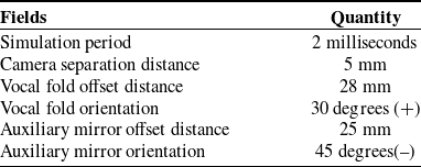
ViSP was used for simulation in C++ SDK, and graphs were plotted with Octave. Table II shows parameters used during the simulation period.
Table II. Simulation parameters.
As actual geometry of the vocal fold is not needed in the controller, since it is implicitly included in the desired and current laser spot position, we simplified the simulation of the vocal fold to a simple planar patch.

Figure 7. Simulated set-up.

Figure 8. (a) Image. (b) Error versus time. (c) Mirror velocity.

Figure 9. (a) Left image. (b) Right image. (c) Error versus time. (d) Mirror velocity.
Figure 7 shows the simulation setup used. Where point $\boldsymbol{{S}}$
corresponds to the laser spot position on the vocal fold. Vector
$\boldsymbol{{S}}$
corresponds to the laser spot position on the vocal fold. Vector $\boldsymbol{{u}}$
is a unit vector in the direction of a laser beam,
$\boldsymbol{{u}}$
is a unit vector in the direction of a laser beam, $\boldsymbol{{d}}$
is the shortest distance from the centre of the micro-mirror to the plane of the auxiliary mirror. Vector
$\boldsymbol{{d}}$
is the shortest distance from the centre of the micro-mirror to the plane of the auxiliary mirror. Vector $\boldsymbol{{u}}_2$
is the reflected unit vector of
$\boldsymbol{{u}}_2$
is the reflected unit vector of $\boldsymbol{{u}}$
,
$\boldsymbol{{u}}$
, $\boldsymbol{{d}}_1$
is the shortest distance between the auxiliary mirror and vocal fold plane, and
$\boldsymbol{{d}}_1$
is the shortest distance between the auxiliary mirror and vocal fold plane, and $\boldsymbol{{z}}\textbf{2}$
is the distance along the reflected laser beam.
$\boldsymbol{{z}}\textbf{2}$
is the distance along the reflected laser beam.

Figure 10. Photography of the experimental setup.

Figure 11. Monocular/ stereoscopic experimental workflow.
This simulation aims to validate the laser monocular visual servoing through an auxiliary mirror, controlled by Eq. (30). Figure 8(a) orange colour asterisk is the laser spot’s initial position, red plus colour is the desired location of spot, and the magenta cross colour is geometric coherence.
The trajectory path shown in the image of Fig. 8(a) marked with a blue line is the laser beam path followed by the steering laser in an image from the initial position to the desired place at hidden parts of the vocal fold. As expected, the trajectory is straight in the image. Error versus time plot shows an exponential convergence, as shown in Fig. 8(b).

Figure 12. (a) Image. (b) Error versus time. (c) Mirror velocity.
4.2. Stereo-view imaging system and auxiliary mirror simulation result in a realistic case
The second simulation implies a stereoscopic imaging system. Thus, a second camera is added to the first simulation setup, and the control in Eq. (34) is applied. The obtained results in Fig. 9(a) and (b) showed that the laser beam’s trajectory path from the initial position to the desired position was straight. Error versus time plot in Fig. 9(c) converged to zero. Similarly, as in Fig. 9(d), mirror velocity had exponential decay.

Figure 13. (a) Left image. (b) Right image. (c) Error versus time. (d) Mirror velocity.

Figure 14. Some experimental images acquired for a single camera system.

Figure 15. Some experimental images acquired for stereo-view imaging system.
5. Experimentation
5.1. Experimental setup
The proposed approaches were validated on the experimental setup shown in Fig. 10. It had two cameras (Guppy pro model: GPF 033B ASG-E0030013 set to work at a frame rate of 25 images per second for a resolution of 640 $\times$
480), a laser source, auxiliary mirror, and an actuated mirror based on a parallel kinematics designed with coplanar axes having triple design, and the platform is driven of three piezo actuators that are located in 120 degrees angles to one another. With the differential drive design, the actuators operate in pairs in a push/pull mode. Two orthogonal rotation axes share a common pivot point. DAC board in a PC generated the analogue input signal; the E-616 PI analogue controller was used to control the actuated mirror’s tip/tilt mirror platform, which caused a change of laser beam direction directed by a laser pointer to the target via an auxiliary mirror. The spot’s position was calculated with respect to the platform centre by a computer (with a program in C++ using the library ViSP http://visp.inria.fr). That computed position was sent to a National Instrument card (NI model: USB-6211 with 250 kS/s) externally installed via a USB connection. This communication was enabled using the Labview platform.
$\times$
480), a laser source, auxiliary mirror, and an actuated mirror based on a parallel kinematics designed with coplanar axes having triple design, and the platform is driven of three piezo actuators that are located in 120 degrees angles to one another. With the differential drive design, the actuators operate in pairs in a push/pull mode. Two orthogonal rotation axes share a common pivot point. DAC board in a PC generated the analogue input signal; the E-616 PI analogue controller was used to control the actuated mirror’s tip/tilt mirror platform, which caused a change of laser beam direction directed by a laser pointer to the target via an auxiliary mirror. The spot’s position was calculated with respect to the platform centre by a computer (with a program in C++ using the library ViSP http://visp.inria.fr). That computed position was sent to a National Instrument card (NI model: USB-6211 with 250 kS/s) externally installed via a USB connection. This communication was enabled using the Labview platform.
The system acquired pixel coordinates through mouse clicks on the image; the user-defined the desired position from which the control algorithm was computed. The corresponding position of the micromanipulator thus servoed laser spot from its initial pose to the desired pose. When the laser finally reached its desired position, user-defined through mouse click the next desired position to be attained by the laser.
5.2. Experimental workflow
Figure 11 shows experimental workflow used for both monocular and stereoscopic cases.
5.3. Single-camera and auxiliary mirror experimental results
Using the setup discussed in Fig. 10, with one camera. The monocular case was validated experimentally, and results obtained in Fig. 12(a) were similar to a simulated case in Section 4.
Figure 12 (b) and (c), error versus time and mirror velocity, respectively, followed exponential decay to reach desired positions, leading to convergence.
5.4. Stereo-view imaging system and auxiliary mirror experimental results
Experimental validation of stereo-view imaging was performed with the setup discussed in Fig. 10. Indeed, Fig. 13(a) and (b) is straight image trajectory path.
Even though both trajectories were straight but for the right image, the path did not reach the desired target; this could be due to laser spot size differences; hence, their centre of gravity moved slightly during control.
Figure 13(c) and (d), error versus time for each image, both $\boldsymbol{{x}}$
, and
$\boldsymbol{{x}}$
, and $\boldsymbol{{y}}$
error components had exponential decay.
$\boldsymbol{{y}}$
error components had exponential decay.
Figures 14 and 15 show live video screenshots of laser servoing for the conducted experiments.
6. Conclusion
The study shows that vocal fold accessibility improved by seeing through a mirror and servoing surgical laser to reach those hidden portions of the vocal fold. Also, the mirror did not affect the controller. The derived control laws could work in both 2D and 3D paths without any prior knowledge of the scene. They were successfully validated in both simulation and experimentally; in all cases, the laser steering control law showed its ability to operate accurately. The experimental results further demonstrated that the proposed control laws were accurate, fully decoupled with exponential decay of the image errors.
The next stages of this study will involve adapting the controller to work under different conditions, for instance, in the influence of perturbations and experimenting on a vocal fold mock-up.
Acknowledgement
This work was supported by the Fondation Charles Defforey – Institut de France through its Grand Prix Scientifique 2018.
Conflicts of Interest
Nicolas Andreff holds a minor share in the capital of Amarob Technologies. All other authors do not have any conflict of interest.
Financial Support
None.
Ethical Considerations
None.
Authors’ Contributions
Odira Japheth Ka’pesha is the main author, and all other are coauthors.


 Open access