


INTRODUCTION
Ocean sediments from the midlatitudes of the North Atlantic record the occurrence of “armadas” of icebergs in proxies such as the ice-rafted debris (IRD). The occurrence of these events that displaced the discharge of detrital material from icebergs to unusually south latitudes are known as Heinrich events, named after the scientist who first identified them and related them to the climate changes associated with them (Heinrich, Reference Heinrich1988). Heinrich events occurred during glacial periods of the Quaternary and had durations of several hundred years to a few millennia, during which the climate in most regions of the Northern Hemisphere typically shifted to significantly colder and/or drier conditions (e.g., McManus et al., Reference McManus, Oppo and Cullen1999; Wang et al., Reference Wang, Cheng, Edwards, An, Wu, Shen and Dorale2001; North Greenland Ice Core Project Members, 2004). The origin of these climate changes involves complex interactions between continental ice and ocean dynamics, with icebergs being a consequence rather than a cause (Barker et al., Reference Barker, Chen, Gong, Jonkers, Knorr and Thornhalley2015). Additionally, the duration of these exceptional cold and arid climate conditions is not limited to the periods when IRD is recorded in ocean sediments (Hemming, Reference Hemming2004; Barker et al., Reference Barker, Chen, Gong, Jonkers, Knorr and Thornhalley2015). Therefore, when focusing on the climate changes related to these events rather than the oceanographic phenomenon in particular, it is more accurate to use the term “Heinrich stadials,” hereafter referred as HSs or HS when referring a singular stadial. Not all sites record a drop in temperature in relation to a HS, and in those sites where negative thermal anomalies were identified, their magnitude is not homogeneous. Different proxies from ocean sediments in mid- and high-latitude sites often record thermal anomalies of several degrees (e.g., Martrat et al., Reference Martrat, Grimalt, Shackleton, de Abreu, Hutterli and Stocker2007). Paleotemperature estimations from continental proxies are not calculated as straightforwardly as estimations from ocean sediments, although a conservative approximation is to extend the sea-surface thermal anomalies to land as supported by climate models (e.g., Pedro et al., Reference Pedro, Jochum, Buizert, He, Barker and Rasmussen2018), keeping in mind at all times the limitations of this assumption.
Temperature in caves is a critical parameter for the cave seasonal dynamics, affecting processes such as cave air ventilation or speleothem growth rates (Spötl et al., Reference Spötl, Fairchild and Tooth2005; Banner et al., Reference Banner, Guilfoyle, James, Stern and Musgrove2007; Kowalczk and Froelich, Reference Kowalczk and Froelich2010). Potentially, changes in temperature also have significant impacts on the underground biota (Mammola et al., Reference Mammola, Piano, Cardoso, Vernon, Domínguez-Villar, Culver, Pipan and Isaia2019) and affect the preservation of cave art (Bourges et al., Reference Bourges, Genthon, Genty, Lorblanchet, Mauduit and D'Hulst2014). During the precipitation of speleothems, temperature is a key control on the fractionation of isotopes or the partition of trace elements (Epstein et al., Reference Epstein, Buchsbaum, Lowenstam and Urey1953; Huang and Fairchild, Reference Huang and Fairchild2001). Consequently, changes in cave air temperature are potentially a significant factor affecting the interpretation of the geochemical records in terms of climate changes (McDermott, Reference McDermott2004; Fairchild and Treble, Reference Fairchild and Treble2009). Cave temperature is especially important in areas where permafrost conditions above the cave affect the flow of seepage water (Genty et al., Reference Genty, Blamart, Ouahdi, Gilmour, Baker, Jouzel and Van-Exter2003) or cause the formation of cryogenic carbonates (Žák et al., Reference Žák, Urban, Cilek and Hercman2004). Also, temperature is of key importance in caves with ice or snow accumulations (Luetscher et al., Reference Luetscher, Lismonde and Jeannin2008). Despite the critical role that temperature has in caves, there are only a limited number of studies on the transfer of climate changes to caves or tunnels (Perrier et al., Reference Perrier, Le Mouël, Poirier and Shnirman2005; Domínguez-Villar et al., Reference Domínguez-Villar, Lojen, Krklec, Baker and Fairchild2015). Beyond cave entrances, where external air has a strong influence due to enhanced air advection (Wigley and Brown, Reference Wigley, Brown, Ford and Cullingford1976; Smithson, Reference Smithson1991), most cave interiors record a limited thermal variability, with temperature values very close to the annual average temperature recorded on the surface over the cave (Moore Reference Moore1964; Moore and Sullivan, Reference Moore and Sullivan1964). For those caves that record little thermal variability, the physical mechanism that transfers heat from the surface to the cave is in most cases thermal conduction (Cropley, Reference Cropley1965; Moore and Sullivan, Reference Moore and Sullivan1978). Exceptions to the general pattern are found in caves where dynamic air currents circulate throughout the cavity or there are significant water streams (Kranjc and Opara Reference Kranjc and Opara2002; Covington et al., Reference Covington, Luhmann, Gabrovšek, Saar and Wicks2011). In these exceptions, advection and radiation are more efficient mechanisms than conduction for transferring heat. Seasonal cave ventilation affects the air temperature in most caves, although the amplitude of the seasonal thermal anomalies is often very limited (e.g., Milanolo and Gabrovšek, Reference Milanolo and Gabrovšek2009). In these cases, the background temperature and the thermal amplitude of the seasonal anomalies are still controlled by thermal conduction, despite advection partially contributes to the variability of the thermal signal (Domínguez-Villar, Reference Domínguez-Villar, Fairchild and Baker.2012; Domínguez-Villar et al., Reference Domínguez-Villar, Lojen, Krklec, Baker and Fairchild2015).
The transport of heat from the external atmosphere to the cave by conduction has two main effects on cave air temperature: (1) The magnitude of thermal anomalies recorded in the external atmosphere is reduced with depth. As a result of the progressive attenuation of thermal anomalies with depth, seasonal cycles transferred by conduction are completely filtered out at 20 m below the surface (Pollack and Huang, Reference Pollack and Huang2000), although the thermal anomalies of more durable thermal cycles continue their propagation to deeper sections of karst. (2) The thermal signal from the surface takes some time to be transferred to a certain depth; consequently, cave temperature signals lag those from the exterior (Cropley, Reference Cropley1965; Moore and Sullivan, Reference Moore and Sullivan1978; Badino, Reference Badino2004). Thermal signals are transferred underground as waves characterized by particular periods, amplitudes, and phase shifts (Smerdom and Stieglitz, Reference Smerdon and Stieglitz2006). Although the record of surface air temperature (SAT) in nature is more complex than simple waves, every signal can be decomposed into a series of independent waves or harmonics, and those simple waves are transferred underground. The propagation velocities underground depend on the period of the harmonic (Villar et al., Reference Villar, Fernández, Quindos, Solana and Soto1983); for example, thermal anomalies associated with annual cycles are transferred to a certain depth faster than those anomalies associated with 11 yr cycles. The complexity of thermal conduction has limited the study of underground thermal conduction to recent decades or centuries (e.g., Perrier et al., Reference Perrier, Le Mouël, Poirier and Shnirman2005; Pollack et al., Reference Pollack, Smerdon and van Keken2005; Beltrami et al., Reference Beltrami, González-Rouco and Stevens2006), and studies that consider climate changes with cycles of thousands of years are rare (Beltrami et al., Reference Beltrami, Mathatoo, Tarasov, Rath and Smerdon2014). However, when studying the long-term evolution of cave microclimate in detail, or when interpreting proxy records from speleothems that cover periods of thousands of years, the impact of long-term changes in cave temperature should not be ignored.
Although the stable air temperature of many cave interiors is similar to the mean annual temperature measured outside the cave, the coupling between the annual SAT and the cave air temperature is often not perfect due to multiple causes (Beltrami and Kellman, Reference Beltrami and Kellman2003; Domínguez-Villar et al., Reference Domínguez-Villar, Fairchild, Baker, Carrasco and Pedraza2013b; Cuthbert et al., Reference Cuthbert, Rau, Andersen, Roshan, Rutlidge, Marjo and Markowska2014). Additionally, because a transit time is required for thermal anomalies recorded at the surface to be transferred underground by conduction, lags are often significant at interannual timescales, enhancing the thermal decoupling. This thermal decoupling has significant impact on speleothem δ18O records (Domínguez-Villar et al., Reference Domínguez-Villar, Fairchild, Baker, Carrasco and Pedraza2013b), one of the most commonly used proxies in speleothem paleoclimate research. Fractionation of oxygen isotopes that are involved in the formation of speleothems is deeply impacted by temperature (Lachniet, Reference Lachniet2009). In midlatitudes, the empirical fractionation factors of water condensation and equilibration with the atmosphere often have a similar magnitude and different sign than the fractionation under equilibrium conditions that takes place during the precipitation of calcite in caves. For this reason, in midlatitude caves, temperature is often neglected as a significant control on the speleothem δ18O record, and most of its variability is assumed to originate from changes in the isotope composition of drip water (e.g., Domínguez-Villar et al., Reference Domínguez-Villar, Wang, Cheng, Martín-Chivelet and Edwards2008; Rossi et al., Reference Rossi, Bajo, Lozano and Hellstrom2018). However, in other midlatitude cave sites, these fractionation factors do not fully counteract each other, and large temperature changes such as those from the Pleistocene are expected to have a significant impact on the speleothem δ18O records (Wainer et al., Reference Wainer, Genty, Blamart, Daëron, Bar-Matthews, Vonhof and Dublyansky2011). Therefore, cave temperature control should be carefully evaluated when studying speleothem δ18O records from midlatitude sites.
Here we provide a theoretical model that transfers the thermal anomaly of a typical HS to a series of caves located at different depths. The model is based on the current knowledge of heat conduction in karst regions, which was previously validated with observations in real caves (Domínguez-Villar et al., Reference Domínguez-Villar, Fairchild, Baker, Carrasco and Pedraza2013b, 2015). Because conduction is the main mechanism to transfer thermal anomalies to the inner part of most caves, the conclusions of this study are transferable to a wide range of real caves. The differences in amplitude and lag time between external and cave thermal signals are also used to evaluate the impact in one of the most commonly used proxies in speleothem paleoclimate research: the ratio of oxygen isotopes (δ18O). The findings of this research have important implications for multiple fields of research such as paleoclimate based on speleothems, cave art conservation, ecological evolution in caves, human and/or faunal evolution, long-term changes in cave microclimate, long-term history of mountain karst aquifers, and the evolution of cave processes (such as modifications in the formation of speleothems, preservation of ice or snow in caves, etc.).
METHODS
Surface air temperature
Although we aim to provide realistic parameters to reproduce climate changes related to HSs, this is a theoretical study and does not focus on a particular location or HS. The magnitude and duration of the modeled HS considered data from the North Atlantic off the Iberian Peninsula and the Mediterranean during the Late Pleistocene (Cacho et al., Reference Cacho, Grimalt, Pelejero, Canals, Sierro, Flores and Shackleton1999; Pérez-Folgado, et al., Reference Pérez-Folgado, Sierro, Flores, Cacho, Grimalt, Zahn and Shackleton2003; Essallami et al., Reference Essallami, Sicre, Kallel, Labeyrie and Siani2007; Martrat et al., Reference Martrat, Grimalt, Shackleton, de Abreu, Hutterli and Stocker2007; Castaneda et al., Reference Castaneda, Schefuss, Patzold, Damste, Weldeab and Schouten2010; Voelker and de Abreu, Reference Voelker, de Abreu, Rashid, Polyak and Mosley-Thompson2011). The hypothetical HS that we reproduce does not consider HSs that occurred during terminations, as their duration, evolution, and climate conditions often differ from HSs that occur during full-glacial climate conditions (e.g., Denton et al., Reference Denton, Broecker and Alley2006; Domínguez-Villar et al., Reference Domínguez-Villar, Vázquez-Navarro, Krklec, Lojen, López-Sáez, Dorado-Valiño and Fairchild2020). We assume that the continents and sea surface recorded similar thermal anomalies. Alkenone derived sea-surface temperature reconstructions were preferred as paleotemperature records, as thermal histories based on fossil assemblages provided inconsistent results in the different regions considered. The modeled HS lasts 1000 yr and has a thermal anomaly of 4°C. The background temperature outside the HS is set in our model to 8°C. We selected this value because we assumed that the cave would be several degrees warmer during interglacial conditions. Thus, during interglacial conditions the temperature of our hypothetical caves would be within the current range of annual average temperatures observed in wide regions of western and southern Europe. Additionally, the selected background temperature does not cause underground freezing during the modeled HS.
The SAT is constructed from a basic wave and up to five of its harmonics to produce a square-like wave. Every wave is characterized by its period, amplitude, and wave phase. The computation of waves as well as the thermal model (see following section) was implemented in a standard spreadsheet program using basic trigonometric, logical, and arithmetic formulas. So, no programming codes were required to perform any calculation in this study. The basic temporal unit of the model is accounted in days, and every time step lasts a month. Every 4 yr, one additional day is added to February to account for leap years. The period of the harmonic with the shorter duration is 181 yr. Thermal anomalies with smaller periods, including the seasonality, are filtered out in this study to emphasize long-term thermal changes. We produce a SAT signal of 5000 yr divided in three different intervals. The SAT signal during the interval from 1000 to 3000 modeled years is the sum of six sinusoidal waves that eventually reproduce the HS from 1500 to 2500 modeled years (Fig. 1). Note that the time scale in all graphs is in modeled years and not in years before present. Consequently, earlier events occur at the left of the graphs and subsequent events to the right. We also provide a background thermal variability before and after the interval from 1000 to 3000 modeled years. In these earlier and later intervals, the SAT signal is composed of only two of the harmonics used to construct the HS signal. This background thermal variability is introduced for the thermal history to be more realistic and to visualize how the HS anomaly interacts underground with earlier and subsequent thermal changes.

Figure 1. Surface atmosphere temperature (SAT) signal considered in the model. The 5000 yr modeled are divided into three intervals. Between 1000 and 3000 modeled years, the record results of the sum of six sinusoidal signals that reproduce a common thermal anomaly during Heinrich stadials. During the previous and subsequent intervals, the record is composed of the sum of two sinusoidal signals that provide background variability. Notice that the timescale is reported as modeled years and not as years ago.
Underground transfer of the SAT
We used a one-dimensional model in which the SAT signal is transferred underground by thermal conduction exclusively. The model assumes a homogeneous infinite half-space with uniform thermal diffusivity. It applies only to caves and karst terrains in the vadose zone, where the phreatic level is deep enough not to interfere with the thermal regime of considered depths. The model was applied to four hypothetical caves located at different depths. The term “depth” is used in this paper for simplicity, although in every case we refer more specifically to the thickness of bedrock above the cave. The selected caves are located 10, 50, 100, and 500 m underground, which covers most cave settings in vadose karsts and is enough to illustrate the importance of the cave depth for the transfer of thermal anomalies. Some alpine caves (i.e., located under high-elevation ranges) can exceed the range of depths here considered. However, at millennial timescales, climate or environmental changes at the surface have a negligible impact on the temperature transferred by conduction to such deep caves, and the thermal consequences would be similar to the ones described in our deeper scenario. Once the thermal signal is conducted from the surface to the ceiling and walls of the cave, the air temperature in the gallery assimilates the temperature of the host rock mainly by radiation in a quick process (Guerrier et al., Reference Guerrier, Doumenc, Roux, Mergui and Jeannin2019). We assume that our modeled caves have no significant water streams and that they have a limited air advection that is not enough to disturb the underground host rock temperature signal. The geothermal gradient and the thermal gradients found in the vadose zone of karst as a result of adiabatic gradients, vertical water flow, and latent heat exchanges are not considered here (Badino, Reference Badino1995; Luetscher and Jeannin, Reference Luetscher and Jeannin2004). In the case of shallow caves, these are negligible controls, and in deep alpine caves, they only produce limited and systematic shifts in absolute temperature (Domínguez-Villar, Reference Domínguez-Villar, Fairchild and Baker.2012).
The thermal signal of every harmonic is transferred underground, and the anomalies are added together according to Eq. 1, where Tz is the underground air temperature at depth z (measured in °C), Az is the amplitude of each signal recorded at the depth z for every wave (measured in °C), t is the time (measured in days), P is the period of each wave (measured in days), ɛ is the wave phase of each wave (measured in radians from 0 to 2π), and Φz is the lag time of each wave at the depth z.

The value of Az is calculated from the attenuation of the amplitude (aA), a parameter obtained for every wave at particular depths from Eq. 3, and the amplitude that every wave has at the surface (As).


The Φz values are calculated from the wave vector (k) measured in radians per meter and the depth measured in meters according to Eq. 4. The k values are calculated according to Eq. 5 from the period of every wave and the thermal diffusivity (κ), a parameter taken from the karst thermal conduction literature (Domínguez-Villar et al., Reference Domínguez-Villar, Fairchild, Baker, Carrasco and Pedraza2013b).


We have implemented our thermal model in two different scenarios. The first scenario assumes thermal coupling between SAT and ground temperature and represents caves with a forest cover above the cave that did not change significantly as a result of the climate changes associated with the HS. Good examples of this scenario are sites where the geographical settings act as refugia for trees regardless of the ecological changes taking place in response to the HS in areas proximal to the site. The second scenario assumes a variable thermal coupling between SAT and ground temperature related to changes in the vegetal canopy over the cave site. The changes in thermal coupling conditions are the ecological response to the climate change associated with the HS, because the microclimate under different vegetal canopies impacts the coupling of SAT and ground temperature (Domínguez-Villar et al., Reference Domínguez-Villar, Fairchild, Baker, Carrasco and Pedraza2013b). In this second scenario, we assume an annual thermal decoupling between SAT and the ground temperature of 2°C that is applied only during the HS interval. This implies that before and after the HS, surface air and ground temperatures are coupled and no thermal shift is applied. Thus, under this scenario, the change to a more open landscape over the hypothetical caves during the HS (Combourieu-Nebout et al., Reference Combourieu-Nebout, Turon, Capotondi, Londeix and Pahnke2002; Brauer et al., Reference Brauer, Allen, Mingram, Dulski, Wulf and Huntley2007; Fletcher and Sanchez-Goñi, Reference Fletcher and Sánchez-Goñi2008; Camuera et al., Reference Camuera, Jiménez-Moreno, Ramos-Román, García-Alix, Toney, Scott Anderson and Jiménez-Espejo2019) results in a mean annual ground temperature 2°C warmer than the mean annual SAT, limiting the impact of the HS on the underground thermal anomaly during the HS.
Oxygen isotope fractionation
We use SAT and Tz signals to calculate an isotope model that evaluates the impact of temperature on the speleothem δ18O records. This model considers two fractionation events: first at the moment of occurrence of atmospheric precipitation, and second, when calcite is formed from the drip-water solution. The so-called temperature effect that takes place during the formation of rainfall (Dansgaard, Reference Dansgaard1964) is based on empirical relationships between rainfall δ18O values and SAT. Isotope fractionation that is temperature related occurs during condensation of rain droplets, as well as during the equilibration of rainwater with the atmospheric moisture (Gat, Reference Gat2010). The ratio between rainwater δ18O (δ18Orw) and SAT in midlatitude sites has a positive relationship, although its magnitude is slightly variable from site to site (Rozanski et al., Reference Rozanski, Araguás-Araguás, Gonfiantini, Swart, Lohmann, McKenzie and Savin1993). We have selected four relationships between δ18Orw and SAT that cover the range of the observed variability in most midlatitude Mediterranean sites (International Atomic Energy Agency, 2009). These δ18Orw/SAT ratios are 0.23, 0.29, 0.35, and 0.41‰/°C.
Our isotope model also considers a second fractionation event that occurs at the moment of speleothem formation. The hypothetical speleothems are composed of calcite and precipitate under equilibrium conditions. The model assumes that no significant evaporation takes place in the karst system and that the drip water is representative of the annual weighted mean of the δ18Orw values. These assumptions were proved right in temperate sites (Genty et al., Reference Genty, Labuhn, Hoffmann, Danis, Meste, Bourges and Wainer2014; Domínguez-Villar et al., Reference Domínguez-Villar, Lojen, Krklec, Kozdon, Edwards and Cheng2018), although they might not be realistic in some arid environments (Ayalon et al., Reference Ayalon, Bar-Matthews and Sass1998; Cuthbert et al., Reference Cuthbert, Rau, Andersen, Roshan, Rutlidge, Marjo and Markowska2014). Although the model considers an effective mixing of the rainwater in the epikarst above the cave during all months of the year, to limit the complexity of the model, we assume a direct transmission of the mixed rainwater to the drip site. We are aware that a negligible residence time (<1 yr) is an unrealistic assumption for most caves. Typical residence times of drip water measured in caves range from one or several years (e.g., Kluge et al., Reference Kluge, Riechelmann, Wieser, Spötl, Sültenfuß, Schröder-Ritzrau, Niggemann and Aeschbach-Hertig2010) to decades (e.g., Yamada, et al., Reference Yamada, Ohsawa, Matsuoka, Watanabe, Brahmantyo, Maryunami, Tagami, Kitaoka, Takemura and Yoden2008), even when the caves are hundreds of meters under the surface (Chapman et al., Reference Chapman, Ingraham and Hess1992). To remove the high-frequency variability in the thermal records, this study considers only climate signals with periods >180 yr. Therefore, at the scale of this study, even drip waters with residence times of several decades would have limited impact on the variability of the speleothem δ18O records (i.e., <0.2‰). Drip-water temperature is assumed to be mostly influenced by cave air temperature which is controlled by bedrock temperature (Guo et al., Reference Guo, Gong, Yuan, Jiang, Cao, Lin, Lo and Chen2019). The precipitation of calcite is set to have a −0.23‰/°C δ18O–cave temperature relationship for the temperature range explored (Kim and O'Neil, Reference Kim and O'Neil1997; Kim et al., Reference Kim, O'Neil, Hillaire-Marcel and Mucci2007). The chosen thermal relationship agrees within uncertainty with the values found in natural and cave-analog experiments (e.g., Johnston et al., Reference Johnston, Borsato, Spötl, Frisia and Miorandi2013; Hansen et al., Reference Hansen, Scholz, Schöne and Spötl2019). The isotope model reports the isotope anomalies related to temperature changes alone. This implies that changes in δ18Orw values related to controls other than temperature are not considered in the modeled isotope anomalies. However, these speleothem δ18O anomalies highlight and quantify the potential impact of temperature on speleothem δ18O records and are useful for evaluating the role of temperature in speleothem δ18O record interpretations.
RESULTS
Cave temperature models
The temperature signal presented in Figure 1 was transmitted by thermal conduction to the caves located at 10, 50, 100, and 500 m underground assuming a thermal coupling between SAT and ground temperature. The original thermal signal was decomposed in six different waves with their particular periods and amplitudes. Each of these signals is recorded at every modeled cave with a different amplitude and lag time (Fig. 2). The amplitude of the thermal anomalies is exponentially muted with depth. The amplitude of the signals with longer periods is more gradually attenuated, which makes the period, and not so much the thermal anomaly, the key control to record significant thermal anomalies in deep caves. The model results show that the lag time for the SAT to be transferred to the cave also depends on the period of every signal. This is important, because the original anomalies in the SAT signal are recorded in the same cave at different times depending on the periods of the different waves that compose the SAT signal. Another obvious implication of the model is that the depth of the cave is a critical parameter controlling both the amplitude of the thermal anomaly and the lag time in relation to the SAT signal.
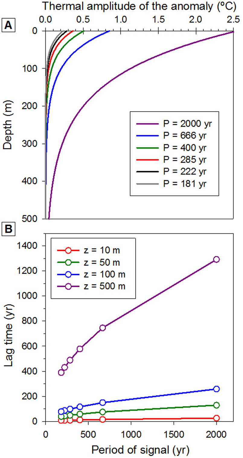
Figure 2. (color online) Underground attenuation of surface atmosphere thermal anomalies and their lag times at selected depths. (A) Underground attenuation of thermal amplitudes of the anomalies for the six signals considered in this study for the atmosphere–soil thermally coupled scenario. P: signal period. The thermal amplitude of the anomaly for every signal is half the difference between the maximum and minimum temperature recorded within a cycle. (B) Lag times modeled for simulated caves at 10, 50, 100, and 500 m in depth (z) as a function of the period of each signal.
The results of transferring the SAT shown in Figure 1 to the hypothetical caves under the first scenario (i.e., thermal coupling between SAT and ground temperature) are shown in Figure 3. The model shows that the temperature signal of the cave located 10 m underground is very similar to the SAT signal, with only some decades of delay. Thus, the background temperature of 8°C cools down on average to 4°C temperature during the HS in both the SAT and 10-m-deep cave temperature records. However, caves located at 50 and 100 m underground already show important attenuations of the maximum thermal amplitude recorded in the caves. Thus, the cave located at a depth of 100 m records a minimum temperature around 6°C in response to the HS. Not just the amplitude of the anomaly, but also the structure of the HS is modified in the cave thermal signal. The different structure of the thermal signal in the cave is caused by the variable periods of the waves that form the SAT signal, which reflect different transit times until they are recorded in the cave. Because the temperature recorded at the cave is the sum of all the waves at a particular moment, the result is an asymmetrical thermal signal with minimum temperature toward the end of the HS. The cave located at a depth of 500 m records a very flat temperature signal despite the existence of a 4°C thermal anomaly on the surface over the cave during the HS. The inset graph within Figure 3 shows the cave air temperature at 500 m in a different scale to display the amplitude and structure of the thermal anomaly related to the HS. Only the wave with the period of 2000 yr lasts long enough to be recorded at this depth, while all other waves are completely muted before reaching the cave, which explains why this anomaly looks like a simple sinusoidal signal. Despite the 4°C of anomaly outside the cave in relation to the HS, less than 0.1°C change is recorded in the cave located at 500 m underground. In addition, the lag time of the 2000 yr period anomaly exceeds 1000 yr at this depth, and consequently, the very small thermal anomaly recorded in the cave occurs when the HS outside the cave has already ended.

Figure 3. (color online) Temperature recorded underground in karst terrains at different depths in response to the surface atmosphere temperature (SAT) signal in an atmosphere–soil thermally coupled scenario. This scenario considers no change in vegetation cover over the cave during the Heinrich stadial. The inset graph shows the temperature record at the depth of 500 m with a different thermal scale to allow visualization of the lag time and structure of the signal.
The results of transferring the SAT shown in Figure 1 to the hypothetical caves under the second scenario (i.e., there is thermal decoupling of 2°C between SAT and ground temperature limited only to the HS) are shown in Figure 4. The temperature transferred underground is the ground-surface temperature and not the SAT. Consequently, changing environmental conditions such as the vegetal cover over the cave modifies the coupling conditions up to several degrees. This scenario assumes that a more open landscape develops over the cave during the HS interval compared with the earlier and later intervals defined in Figure 1. The change in landscape over the cave sites reduces the thermal anomaly to be transferred underground to half the value in the SAT. Apart from the amplitude, the structure of the signals is exactly the same as in the coupled scenario.

Figure 4. (color online) Temperature recorded underground in karst terrains at different depths in response to the surface atmosphere temperature (SAT) signal in an atmosphere–soil thermally decoupled scenario. This scenario considers a change in vegetation cover over the cave site during the Heinrich stadial. The inset graph shows the temperature record at the depth of 500 m with a different thermal scale to allow visualization of the lag time and structure of the signal.
Speleothem δ18O models
We use the results of the cave temperature records of both scenarios and the SAT record to evaluate the thermal impact on speleothem δ18O records as a result of the HS. A first event of isotope fractionation occurs in the atmosphere above the cave. The isotope models use four different δ18Orw/SAT ratios that account for the impact of temperature during fractionation in the atmosphere, covering most of the variability found in temperate Mediterranean sites. Because the ratios are always positive, there is a direct correlation between δ18Orw and SAT. The second fractionation event considered in this model is also temperature dependent and occurs at the moment of speleothem calcite precipitation. During the precipitation of calcite, the oxygen isotopes have a negative relationship with temperature. We considered this value to be constant due to the limited thermal variability in caves.
The impact of temperature in the cave after these two fractionation events is shown in Figure 5 for the first scenario (i.e., thermal coupling between SAT and ground temperature). The results show that the thermal changes related to HS under the boundary conditions constrained in this model have variable impact on caves at different depths. Both the cave depth and the δ18Orw/SAT ratios are important parameters that determine the significance of the impact that temperature changes during HS have on speleothem δ18O records. In caves located 10 m from the surface and having a δ18Orw/SAT ratio of +0.23‰/°C, the thermal impact on speleothem δ18O records is mostly indistinguishable from analytical uncertainties. At the other extreme, caves located 500 m underground and having a δ18Orw/SAT ratio of +0.41‰/°C are capable of recording a thermal impact in their speleothem δ18O records of >1.6‰ during the HS. The attenuation of the temperature anomalies with depth causes thermal gradients with SAT that have an impact on the speleothem δ18O records. This impact is enhanced in deeper caves, as their temperature is less affected by changes in SAT. When significant speleothem δ18O anomalies related to the HS result from the model, the speleothem δ18O signals are generally shifted toward more negative values. The lag times related to the transfer of thermal signal underground also impact the structure of the isotope anomalies recorded in the speleothems, which is more obvious in the modeled caves located 50 and 100 m underground. During the HS, the speleothem δ18O anomaly is not constant in response to the progressive change in cave temperature. Additionally, at the end of the HS, the caves 50 and 100 m underground record a shift in their modeled speleothem δ18O records toward less-negative δ18O values. This positive δ18O anomaly is a product of the lag times and can be >0.5‰ at its peak, lasting several decades.

Figure 5. (color online) Impact of surface and underground temperature changes in calcite speleothem δ18O records (reported as δ18O anomalies) for caves at different depths (z) in an atmosphere–ground surface thermally coupled scenario. This scenario implies no changes in the vegetation cover over the cave as a result of the Heinrich stadial (HS). Isotope calculations consider that during the precipitation of calcite, fractionation occurs under equilibrium conditions. The model assumes that drip-water isotope composition only changes due to changes in surface atmosphere temperature (SAT). The model is implemented for four cases in which the relationship between rainwater δ18O values and the SAT (δ18Orw/SAT ratio) during fractionation of oxygen isotopes in the atmosphere differs. (A) Case of δ18Orw/SAT ratio = +0.23‰/°C; (B) case of δ18Orw/SAT ratio = +0.29‰/°C; (C) case of δ18Orw/SAT ratio = +0.35‰/°C; and (D) case of δ18Orw/SAT ratio = +0.41‰/°C. The variability of the input signal of δ18Orw anomaly in each of the four cases coincides with the variability of the δ18Occ signal at the depth of 500 m, because there is no significant change in temperature at this depth as result of the changes in SAT during the HS.
The speleothem δ18O model under the second scenario (i.e., thermal decoupling of 2°C between SAT and ground temperature limited only to the HS) shows either remarkable differences or nearly identical results compared with the first scenario, depending on the depth of the cave (Fig. 6). The temperature of the cave located 500 m underground is almost unaffected by SAT or the changes in vegetation, and consequently, the outputs of the speleothem δ18O model are nearly identical to those of the first scenario. On the other hand, the temperature of the cave located 10 m underground changes the most as a result of the variable thermal decoupling, and its speleothem δ18O record does too. Under the variable decoupling scenario, the cave 10 m deep has negative speleothem δ18O anomalies ranging from 0.4 to 1.2‰ during the HS depending on the δ18Orw/SAT ratio considered. The caves located 50 and 100 m underground also record slightly more-negative speleothem δ18O anomalies during the HS under this second scenario. The impact of lag times on the speleothem δ18O records is less obvious compared with the first scenario, because thermal anomalies are reduced. However, all the speleothem δ18O signal structures reported in the first scenario are also recorded here, despite their differences in amplitude.

Figure 6. (color online) Impact of surface and underground temperature changes in calcite speleothems δ18O records (reported as δ18O anomalies) for caves at different depths (z) in a variable atmosphere–ground surface thermally decoupled scenario. This scenario implies changes in the vegetation cover over the cave as a result of the Heinrich stadial (HS). Isotope calculations consider that during the precipitation of calcite, fractionation occurs under equilibrium conditions. The model assumes that drip-water isotope composition only changes due to changes in surface atmosphere temperature (SAT). The model is implemented for four cases in which the relationship between rainwater δ18O values and the SAT (δ18Orw/SAT ratio) during fractionation of oxygen isotopes in the atmosphere differs. (A) Case of δ18Orw/SAT ratio = +0.23‰/°C; (B) case of δ18Orw/SAT ratio = +0.29‰/°C; (C) case of δ18Orw/SAT ratio = +0.35‰/°C; and (D) case of δ18Orw/SAT ratio = +0.41‰/°C. The variability of the input signal of δ18Orw anomaly in each of the four cases coincides with the variability of the δ18Occ signal at the depth of 500 m, because at this depth there is no significant change in temperature as result of the changes in SAT or vegetation cover during the HS.
DISCUSSION
Impact of millennial-scale SAT changes in caves
We have applied our thermal conduction model to two scenarios that consider coupling and variable decoupling of the SAT and ground temperature. There is a possible third scenario that we have not considered yet, in which the ground records a systematic temperature shift compared with SAT. This scenario implies that there is a temperature difference between the ground and the atmosphere, but the long-term mean of this value does not change. The thermal variability under this constantly decoupled scenario will be identical to that of the coupled scenario, although the absolute values will differ as much as the magnitude of the decoupling. The same absolute differences will be transferred underground to the cave, whereas the cave temperature variability will be exactly the same as in the coupled scenario. This third scenario is likely to occur, for example, in caves under a rocky terrain in which trees or shrubs are unlikely to grow independent of the climate conditions. In the second scenario, we have assumed a variable thermal decoupling to account for changes in the landscape over the cave. Vegetation cover is a major control on the coupling conditions between SAT and ground-surface temperature (Lewis and Wang, Reference Lewis and Wang1998). However, other controls such as snow cover, irradiation, or evaporation are potentially also significant (Beltrami and Kellman, Reference Beltrami and Kellman2003; Smerdon, et al., Reference Smerdon, Pollack., Cermak, Enz, Krel, Safanda and Wehmiller2006; Yazaki et al., Reference Yazaki, Iwata, Hirota, Kominami, Kawakata, Yoshida, Yania and Inoue2013). We have selected a decoupling value of 2°C, which is less than the annually averaged thermal difference between SAT and the ground temperature under Mediterranean forest and grassland (Domínguez-Villar et al., Reference Domínguez-Villar, Fairchild, Baker, Carrasco and Pedraza2013b). This muted decoupling value was selected to account for the additional impact of other potential controls such as the increase of snow cover and the decreased evaporation during the HS or the diminished irradiance during glacial times compared with the present.
The model shows that the temperature of cave interiors can differ by several degrees from the long-term SAT. These long-term thermal gradients are more pronounced in deeper caves. This creates a thermal gradient between the cave and the external atmosphere that affects the cave ventilation by changing the gradient of air densities (de Freitas et al., Reference de Freitas, Littlejhon, Clarkson and Kristament1982; Kowalczk and Froelich, Reference Kowalczk and Froelich2010). This gradient is not constant but fluctuates, as we have to consider that our thermal model has filtered out the seasonality. Therefore, every year the SAT is expected to oscillate above and below the cave temperature, forcing different ventilation modes. Nevertheless, this long-term thermal gradient is expected to affect the intensity and duration of seasonal ventilation modes. The seasonal period of enhanced ventilation that occurs when SAT is below the cave interior temperature is expected to last longer and be more vigorous as a consequence of cave temperature being warmer than the mean annual SAT. On the other hand, the season of diminished ventilation is expected to be shortened. The extended seasonal period of enhanced ventilation caused by the long-term warmer cave temperature is expected to favor the growth rate of speleothems (Banner et al., Reference Banner, Guilfoyle, James, Stern and Musgrove2007; Boch et al., Reference Boch, Spötl and Frisia2011). However, other key controls on speleothem growth rate are drip rate and calcium activity in the drip solution (Baker et al., Reference Baker, Genty, Dreybrodt, Barnes, Mockler and Grapes1998), which under dry conditions are likely to counteract or even surpass the impact of enhanced ventilation on speleothem growth rate. So, despite the expected changes in ventilation in some caves in relation to HS, no general pattern on the changes in speleothem growth rate can be predicted, as local conditions may determine the dominant control.
Cave microclimate and underground ecological environments can also be potentially affected by the extended and more dynamic seasonal ventilation during HSs. A significantly drier climate may impact the water availability in the cave, which together with the enhanced advection due to the more dynamic ventilation, is potentially capable of decreasing seasonally the relative humidity of the cave interior. When cave atmosphere is not close to saturation in water (i.e., relative humidity clearly below 100%), clay and other particles are easier to move as aerosols, and dust can be observed in the cave atmosphere (Dredge et al., Reference Dredge, Fairchild, Harrison, Fernandez-Cortés, Sanchez-Moral, Jurado and Gunn2013) and potentially recorded in the trace elements of speleothems. The occurrence of moist–dry cycles on cave walls as a result of unsaturated cave air in water can favor the conditions for weathering of carbonates (Karbowska-Berent, Reference Karbowska-Berent, Koestler, Koestler, Charola and Nieto-Fernandez2003; Dreybrodt et al., Reference Dreybrodt, Gabrovšek and Perne2005; Krklec et al., Reference Krklec, Domínguez-Villar, Carrasco and Pedraza2016) and impact the cave ecological niches, having important consequences for the preservation of cave art (Saiz-Jimenez et al., Reference Saiz-Jimenez, Cuezva, Jurado, Fernandez-Crtés, Porca, Benavente, Cañaveras and Sánchez-Moral2011). Evaporation can cause significant changes in growth rate by affecting the saturation index that impacts calcite fabrics and trace elements, as well as controlling the speleothem δ18O and δ13C values (Frisia et al., Reference Frisia, Borsato, Fairchild and McDermott2000; Mickler et al., Reference Mickler, Banner, Stern, Asmerom, Edwards and Ito2004; Fairchild and Treble, Reference Fairchild and Treble2009). Although the water availability in caves has a critical local component, caves under arid and semiarid climates are more likely candidates to be affected by evaporation as a result of HS.
Impact of SAT changes in speleothem isotope records
We used four different constant δ18Orw/SAT ratios in our isotope models. The assumption that a site will have a constant δ18Orw/SAT ratio through time is likely unrealistic. However, little is known yet concerning the long-term changes in the δ18Orw/SAT relationship (Fricke and O'Neil, Reference Fricke and O'Neil1999). Our assumption is still a good approximation to evaluate potential impacts of HS on speleothem δ18O values, keeping in mind the boundary conditions of the model and its limitations when doing interpretations.
We mentioned in the previous section that enhanced ventilation could favor evaporation and consequently affect the speleothem δ18O and δ13C values. However, in the isotope model we present, we are assuming that the caves maintain a saturated atmosphere, preventing the occurrence of kinetic fractionation during calcite precipitation that would affect the speleothem δ18O record. Yet the long-term thermal gradient between the cave and the external atmosphere is expected to affect the ventilation modes, potentially affecting the speleothem δ13C record. The degassing of CO2 from the dissolved inorganic carbon in the solution can be a major control on the speleothem δ13C values for some speleothems (Frisia et al., Reference Frisia, Fairchild, Fohlmeister, Miorandi, Spötl and Borsato2011). In those cases, a shift in the speleothem δ13C record is expected as a result of the thermal changes of the HS independent of the changes in the vegetation cover, soil properties on top of the cave, or the system's carbonate dissolution style. However, the controls affecting speleothem δ13C are site specific, and degassing is not always a major contributor to the speleothem δ13C variability (Mattey et al., Reference Mattey, Lowry, Duffet, Fisher, Hodge and Frisia2008; Dreybrodt and Scholz, Reference Dreybrodt and Scolz2011; Tremaine et al., Reference Tremaine, Froelich and Wang2011; Griffiths, et al., Reference Griffiths, Fohlmeister, Drysdale, Hua, Johnson, Hellstrom, Gagan and Zhao2012). Therefore, although the long-term thermal gradient caused by the HS has the potential to affect speleothem δ13C records, this effect is not expected to have a significant contribution to the δ13C variability of every speleothem.
The results of our isotope model suggest that under equilibrium conditions, the isolated impact of temperature on speleothem δ18O values can be >1.6‰. As many factors affect the δ18Orw values (Lachniet, Reference Lachniet2009), during HS the changes in the hydrological cycle that impact δ18Orw values are not limited to temperature changes. However, our model is not designed to represent the real anomalies that speleothems would record, but the anomalies that could only be attributed to the thermal impact. So the impact of temperature on speleothem δ18O records will be significant only when other controls taken all together will not counteract the thermal effect. Because the δ18O variability associated with HSs and similar cold episodes in temperate Mediterranean speleothems is often <2‰ (Drysdale et al., Reference Drysdale, Zanchetta, Hellstrom, Fallick, McDonald and Cartwright2007; Fleitmann et al., Reference Fleitmann, Cheng, Badertscher, Edwards, Mudelsee, Göktürk and Fankhauser2009; Moreno et al., Reference Moreno, Stoll, Jiménez-Sánchez, Cacho, Valero-Garcés, Ito and Edwards2010; Domínguez-Villar et al., Reference Domínguez-Villar, Carrasco, Pedraza, Cheng, Edwards and Willenbring2013a), it is clear that the temperature effect is likely to be a significant control on the speleothem δ18O records at most sites that share the boundary conditions used in our model.
CONCLUSION
This research has developed a one-dimensional thermal conduction model to show how millennial-scale temperature drops, such as those recorded during HSs in Atlantic and Mediterranean sites, are transferred to caves. The model shows that the depth of the cave and the duration of the anomaly are important controls for the thermal anomaly to be recorded underground. Caves hundreds of meters deep can record little evidence of the HSs temperature changes recorded at the surface. On the other hand, shallow caves are more likely to record significant thermal changes during HSs. A thermal anomaly is progressively attenuated with the increasing depth of the cave, but the recorded thermal signal is also affected by increased delays and more drastic modifications in its structure as a function of depth. The results provided here support that not all caves are in thermal equilibrium with the exterior atmosphere during HSs.
We have also discussed the impact that this thermal disequilibrium may have on different cave dynamics and speleothem proxies. The results support the occurrence of long-term thermal gradients between the caves and the exterior as a consequence of HSs. These gradients are more pronounced in deep caves and less significant in shallow caves. Thermal gradients are likely to cause modifications on the ventilation regime in caves and affect multiple processes, some of them being recorded in speleothems. Although changes in ventilation can affect multiple speleothem proxies, local controls are too important to expect a unitary response in cave systems. However, we can evaluate the impact of temperature during HSs on speleothem δ18O records. The isotope models here reported show that for most temperate and Mediterranean cave sites, the thermal impact of HSs cannot be neglected when interpreting speleothem δ18O records. Therefore, despite the anticipated important modifications of the hydrological cycle affecting δ18Orw values during HS, Pleistocene speleothem δ18O values still record significant changes in relation to temperature alone.
This research has put the focus once more on temperature as a significant control of speleothem isotope records during Pleistocene climate changes. Also, we have demonstrated how the depth of the cave can impact its dynamics and speleothem records. Therefore, we encourage scientists working in paleoclimate research to always report the depths of the caves they are studying.
ACKNOWLEDGMENTS
The lead author of this research (DD-V) received funds from the project “Inter-comparison of Karst Denudation Measurement Methods” (KADEME) (IP-2018-01-7080) financed by Croatian Science Foundation.


 Open access