


1. Introduction
The SkyMapper Southern Survey (SMSS) is obtaining a digital image of the entire Southern hemisphere of the sky. It is designed to reach a depth of 20–22 mag in six optical filters and achieve near-arcsecond-level spatial resolution. The survey started in 2014 with an emphasis on the short-exposure Shallow Survey. Images from the Shallow Survey reach 10 $\sigma$
limits for point sources around 18 mag, and instantaneous six-filter photometry data for over 280 million stars, galaxies, and quasars were published in a first data release (DR1; Wolf et al. Reference Wolf, Onken and Luvaul2018a).
$\sigma$
limits for point sources around 18 mag, and instantaneous six-filter photometry data for over 280 million stars, galaxies, and quasars were published in a first data release (DR1; Wolf et al. Reference Wolf, Onken and Luvaul2018a).
DR1 has already facilitated the discovery of the most luminous quasar currently known (Wolf et al. Reference Wolf, Bian and Onken2018b), while the discovery of the most iron-poor star currently known (Keller et al. Reference Keller2014) was based on commissioning data from SkyMapper. On both topics, further work continues: a paper describing a new large sample of extremely metal-poor stars based on DR1 photometry and low-resolution spectroscopy with the Australian National University (ANU) 2.3 m telescope is nearing completion (Da Costa et al. in preparation), as is a paper discussing the results from high-dispersion spectroscopic follow-up of the most metal-poor star in this sample (Nordlander et al. Reference Nordlander, Bessell and Da Costa2019); similarly, the growing sample of confirmed ultraluminous quasars at $z>4$
has been compiled (Wolf et al. Reference Wolf, Hon and Bian2019b).
$z>4$
has been compiled (Wolf et al. Reference Wolf, Hon and Bian2019b).
DR1 has also helped with discovering extremely metal-poor stars in the Tucana II Dwarf Galaxy (Chiti et al. Reference Chiti, Frebel and Ji2018), with studies of the most metal-poor Galactic globular cluster (Simpson Reference Simpson2018), and with characterising the lowest-mass ultra metal-poor star known (Schlaufman, Thompson, & Casey Reference Schlaufman, Thompson and Casey2018). Many other scientific endeavours in the Southern skies are underway using DR1 data.
This paper now presents the second data release, DR2, which adds, for the first time, long exposures from the SkyMapper Main Survey. The 100 s exposures of the Main Survey provide individually a $1\!-\!3$
mag gain in point source depth and surface brightness sensitivity. By the time the survey finishes, the Southern sky should be imaged to 5
$1\!-\!3$
mag gain in point source depth and surface brightness sensitivity. By the time the survey finishes, the Southern sky should be imaged to 5 $\sigma$
-limits of (20,21,22,22,21,20) mag in the filters (u,v,g,r,i,z), respectively. All SkyMapper magnitudes are in the ABPlease define ‘AB’ if needed. system (Oke & Gunn Reference Oke and Gunn1983).
$\sigma$
-limits of (20,21,22,22,21,20) mag in the filters (u,v,g,r,i,z), respectively. All SkyMapper magnitudes are in the ABPlease define ‘AB’ if needed. system (Oke & Gunn Reference Oke and Gunn1983).
The leap in depth relative to DR1 extends the reach of Galactic archaeology studies in our own Milky Way, such as studies of Blue Horizontal Branch stars, which were limited in distance by the previous shallow DR1 (Wan et al. Reference Wan, Kafle and Lewis2018). Given the enhanced surface brightness sensitivity, DR2 now enables a broad range of work on galaxies, where the previously released Shallow Survey data of DR1 mostly supported studies of the Milky Way and bright quasars. The first example is by Wolf et al. (Reference Wolf, Golding, Onken and Shao2019a), who present colour maps of well-resolved galaxies at low redshift, and discuss how SkyMapper filters help to trace spatio-temporal variations of the star-formation rate in galaxies.
The DR2 Main Survey data set provides nearly full hemispheric coverage in i and z filters (see Figure 1), which will serve, among other purposes, as reference frames for the detection of optical transients related to gravitational-wave events detected with Advanced LIGO, such as the kilonova from the binary neutron star merger GW170817 (e.g., Abbott et al. Reference Abbott, Abbott and Abbott2017; Andreoni et al. Reference Andreoni, Ackley and Cooke2017).
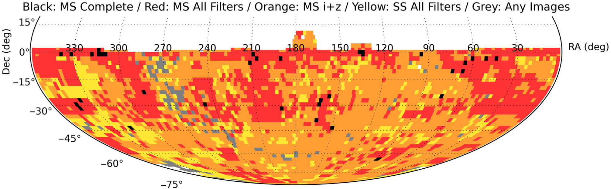
Figure 1. Coverage of SkyMapper DR2, colour-coded to indicate the progress on different fields: (black) complete Main Survey coverage in all six filters; (red) at least one Main Survey image in all six filters; (orange) Main Survey images in iz filters; (yellow) Shallow Survey images in all six filters; (grey) any images. Main Survey images have exposure times of 100 s in each filter, while the Shallow Survey exposures in u,v,g,r,i,z are 40, 20, 5, 5, 10, 20 s, respectively.
This release was made availableFootnote a to Australian astronomers, SkyMapper partners, and their worldwide collaborators on 2019 February 27. The proprietary period is currently expected to last 18 months, after which DR2 will become world-public without restrictions.
This paper is organised as follows: in Section 2, we describe the Main Survey and changes in processing relative to DR1; in Section 3, we describe properties of the DR2 data set; in Section 4, we provide an update on the data access methods; and in Section 5, we discuss the future survey development.
2. Enhancements in DR2
DR2 builds on the Shallow Survey data and processing of DR1 described by Wolf et al. (Reference Wolf, Onken and Luvaul2018a), and we refer the reader to Section 4 of that paper for the details of the image processing and photometric measurements. The primary gain planned for DR2 was the inclusion of deeper images from the Main Survey, as well as more Shallow Survey data. However, we also improve the data products further (as described in the subsections below) by applying stricter cuts on image quality, by removing fringes in iz images, and by using an improved photometric zero-point calibration tied to Gaia DR2.
Main Survey images are always exposed for 100 s, while the Shallow Survey exposure times range from 5 s in g and r filters to 40 s in u-band. The gain in depth is often above the naively expected $\sqrt{t_{\rm exp}}$
factor, as the Shallow Survey images are affected by read noise. Figure 2 compares typical exposures from each survey component side by side, targeting part of the Sculptor galaxy NGC 253 and the open cluster Messier 11.
$\sqrt{t_{\rm exp}}$
factor, as the Shallow Survey images are affected by read noise. Figure 2 compares typical exposures from each survey component side by side, targeting part of the Sculptor galaxy NGC 253 and the open cluster Messier 11.
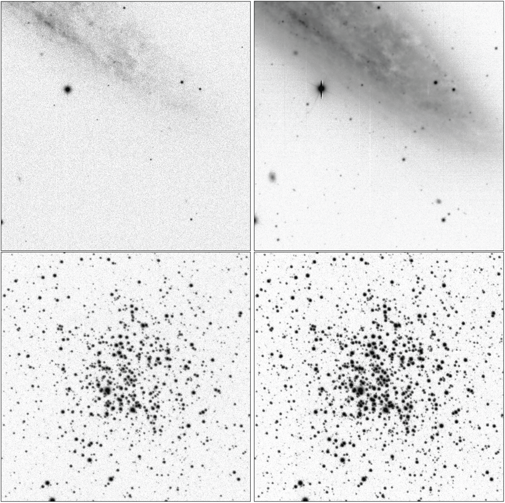
Figure 2. Comparison of image pairs from the two survey components (size 10 $\times\, 10\,\text{arcmin}$
): Shallow Survey (left,
$\times\, 10\,\text{arcmin}$
): Shallow Survey (left, $t_{\rm exp}=5 \ldots 40$
s) and Main Survey (right,
$t_{\rm exp}=5 \ldots 40$
s) and Main Survey (right, $t_{\rm exp}=100$
s). Top: g-band images of the galaxy NGC 253. Bottom: u-band images of the open cluster Messier 11. While the exposure time ratio in g-band is 20, it is only 2.5 in u-band. North is up and East is left.
$t_{\rm exp}=100$
s). Top: g-band images of the galaxy NGC 253. Bottom: u-band images of the open cluster Messier 11. While the exposure time ratio in g-band is 20, it is only 2.5 in u-band. North is up and East is left.
While the saturation magnitude for point sources is typically 10 mag in g and r filters in the Shallow Survey, the factor 20 increase in exposure time in the Main Survey moves it fainter by 3.25 mag. However, the completeness limit of point-source detection, which is on the order of 18 mag in the Shallow Survey, is expected to push fainter by less than that due to increased sky background.
The image data set for DR2 is just like that of DR1—reduced images from each Please spell out ‘CCD’ at first use, if needed. charge-coupled device (CCD) in the mosaic are accessible via an image cut-out service on the SkyMapper website, along with the corresponding mask image. Non-zero values in the mask reflect, for each pixel, one or more of the following issues: 1, non-linear; 4, affected by saturation; 8, affected by cross-talk from the other half of that CCD; 32, a cosmic ray was removed from the pixel; and 64, affected by electronic noise (see Section 2.4). Masked pixels are treated in two ways during the production of photometry: non-linear pixels are interpolated over, while other issues are captured by Source Extractor (version 2.19.5; Bertin & Arnouts Reference Bertin and Arnouts1996) into the parameters IMAFLAGS (the OR-combined values of the mask within the isophotal aperture) and NIMAFLAGS (the number of affected pixels within the isophotal aperture).
The structure of the DR2 data tables is very similar to that of DR1, with a few important modifications described in Section 4. The list of distinct astrophysical objects, and their averaged primary properties, is contained in the master table. The individual photometric measurements from each image are given in the photometry table. The tables describing the observations themselves are organised into an images table containing image-level properties, a ccds table that incorporates CCD-specific information, and a mosaic table that describes the relationship between the CCDs in the mosaic. A set of external catalogues with DR2 cross-matches is also available. The construction of the data tables is described in more detail in Sections 2.6, 3.3, and 3.8.
2.1. Observing strategy and cadence
The observing strategy in the Shallow Survey is very simple: any time a field is targeted, it is observed with a full colour sequence of six filters that is completed within 4 min, if there are no interruptions. The Main Survey, in contrast, has several components that are completed over different visits to a field:
1. For the first long visit, we take a colour sequence that includes three exposures for the filters u and v and one exposure for the remaining filters griz, using the order uvgruvizuv. The sequence is executed as a block and typically completed in 20 min.
2. Additional exposure pairs in the filters g and r are added during dark and grey time; since March 2017 we restricted the gr pairs to dark time, because g-band is our most sensitive filter to moonlight.Footnote b Two gr blocks are collected on different nights and typically executed in 4 min each.
3. Additional iz pairs are executed as 4-min blocks and observed during astronomical twilight (between $-12^{\circ}$
and
$-18^{\circ}$
Sun altitudes) or in bright time, regardless of other progress on the field. Up to three iz pairs are added over the course of the survey.
$-12^{\circ}$
and
$-18^{\circ}$
Sun altitudes) or in bright time, regardless of other progress on the field. Up to three iz pairs are added over the course of the survey.4. The final step is a second colour sequence that is identical to the first.


Owing to this strategy, we obtain near-instantaneous six-filter spectral energy distributions (SEDs) via the colour sequences, and we gain more depth by adding further data when the observing conditions are most suitable. As a result of this strategy, DR2 contains a mix of completion statistics across the hemisphere. Since 2014 November 14, the astronomical twilight time at SkyMapper has been used exclusively for Main Survey iz pairs, which explains why these filters already provide nearly hemispheric coverage with at least one visit. Nearly 33% of the Southern sky is covered with all six filters in the Main Survey, typically including one colour sequence, two gr pairs and some iz pairs, i.e., three exposures per filter. The full data set brings the exposure numbers up to (6,6,4,4,5,5) for the (u,v,g,r,i,z) filters but is only complete for 1% of the hemisphere in DR2.
The resulting cadence of repeat observations also depends on the filter: the colour sequences provide a short-cadence lightcurve in uv consisting of three pairs separated by typically 8 min. Repeat observations of gr pairs and iz pairs take place on separate nights, hence they could be as close as $\sim\! 20$
h, or separated by years. The final colour sequence is typically at least a year after the first colour sequence, so the full spectral energy distribution of faint sources is probed only for long-term variability.
$\sim\! 20$
h, or separated by years. The final colour sequence is typically at least a year after the first colour sequence, so the full spectral energy distribution of faint sources is probed only for long-term variability.
Main Survey exposures have a median separation of 14 d in the filters g and r, and 1 yr in the filters i and z. The distribution of time difference between the first and the second colour sequence has two peaks, at 1 yr and at 1 month (owing to the Lunar period).
While the cadence described above holds for a given SkyMapper field, it does not necessarily apply to every object within the field. Because of the gaps between CCDs within the mosaic (0.5 and 3.2 arcmin between rows, 0.8 arcmin between columns), a dither pattern is been applied for the observations of each visit. For the Main Survey observations in each filter, the nominal pattern of (RA, Dec) offsets from the field centre, in arcmin, is $(-5, -1.7), (-1.7, +5), (+1.7, -5), (+5, +1.7), (-8.6, -8.6), (+8.6, +8.6)$
. The malfunction of various detector controller electronics since October 2017 has led to modifications of the pattern, with step sizes as large as
$(-5, -1.7), (-1.7, +5), (+1.7, -5), (+5, +1.7), (-8.6, -8.6), (+8.6, +8.6)$
. The malfunction of various detector controller electronics since October 2017 has led to modifications of the pattern, with step sizes as large as $12\ \text{arcmin}$
, but only 1% of DR2 data entails such a large offset. For the Shallow Survey, the dither pattern of the first three visits ranges up to
$12\ \text{arcmin}$
, but only 1% of DR2 data entails such a large offset. For the Shallow Survey, the dither pattern of the first three visits ranges up to $5\ \text{arcmin}$
from the field centre, but the subsequent visits apply roughly half-field (
$5\ \text{arcmin}$
from the field centre, but the subsequent visits apply roughly half-field ( $1^{\circ}_{\cdot} 1$
) offsets in each of RA and Dec, in order to yield more homogeneous photometry from the complete data set.
$1^{\circ}_{\cdot} 1$
) offsets in each of RA and Dec, in order to yield more homogeneous photometry from the complete data set.
2.2. Image selection
We started from $\sim160\,000$
images that were observed between 2014 March 15 and 2018 March 14 and processed with our Science Data Pipeline (SDP; Luvaul et al. Reference Luvaul, Onken, Wolf, Smillie, Sebo, Lorente and Shortridge2015; Wolf et al. Reference Wolf, Luvaul, Onken, Smillie, White, Lorente and Shortridge2015). We then selected 121 494 images using the following quality control criteria:
$\sim160\,000$
images that were observed between 2014 March 15 and 2018 March 14 and processed with our Science Data Pipeline (SDP; Luvaul et al. Reference Luvaul, Onken, Wolf, Smillie, Sebo, Lorente and Shortridge2015; Wolf et al. Reference Wolf, Luvaul, Onken, Smillie, White, Lorente and Shortridge2015). We then selected 121 494 images using the following quality control criteria:
1. While the median number of calibrator stars for zero-point determination is over 1 600 per frame, we require at least 6 calibrator stars; only 0.6% of frames have less than 100 stars.
2. We fit linear throughput gradients across our wide field of view to the calibrator stars and reject images with strong gradients. Our mean ensemble gradients are consistent with zero; we require that their slopes do not exceed 0.05 mag per
$2^{\circ}_{\cdot} 3$
width of the field of view in griz filters and no more than 0.1 mag in the uv filters.3. We measure the root mean square (RMS) scatter of zero points among the calibrator stars to identify frames with uneven throughput due to structured cloud or other reasons, and reject frames where the RMS exceeds 0.05 mag in griz filters and 0.12 mag in the uv filters.
4. We determine typical zero points per filter, which drift in time as the telescope optics accumulate dust and reject frames with low throughput, when the loss is on the order of 1 mag or more.
5. We reject frames where the mean point spread function (PSF) has a full-width at half maximum (FWHM) above
$5\ \text{arcsec}$
or elongation (the ratio of semi-major to semi-minor axis lengths) above 1.4.6. We tighten the constraints on the World Coordinate System solutions compared to DR1, such that both corner-to-corner lengths of each CCD are required to be within
$1\ \text{arcsec}$
of the median values for that particular CCD and filter.7. We reject frames with high background and use thresholds ranging from 500 counts for uv filters, irrespective of exposure time, to thresholds of 3 000 counts for Main Survey frames in iz filters.


2.3. Data processing differences
The major improvement in the image processing compared to DR1 is the treatment of fringing in the iz filters. Each filter was investigated with a principal component (PC) analysis to determine the main modes of fringing behaviour [similar procedures have been described by Brooks, Fisher-Levine, & Nomerotski (Reference Brooks, Fisher-Levine and Nomerotski2017) and Bernstein et al. (Reference Bernstein, Abbott and Desai2017)]. We expect the fringes to be a linear combination of patterns, each of which is created by groups of night-sky emission lines that vary separately in intensity. The fringe pattern caused by each independently varying group would thus be represented by a PC. We find that this approach of multiple, independent fringe frames suppresses fringe residuals in SkyMapper images better than using only a mean fringe pattern, i.e. the first PC.
Taking about 5 000 bias- and flat-field-corrected Main Survey images for each filter, the astrophysical objects in each image were removed and a large-spatial-scale background map was created and subtracted. For the final analysis, we chose a subsample of images that were not excessively dense with objects, were free of large numbers of saturated pixels, and had background levels (prior to subtraction) between 250 and 2 500 counts. About 3 000 images per filter, selected independently for each CCD, were run through a PC analysis routine (using the scikit-learn Python module; Pedregosa et al. Reference Pedregosa2011) to produce the top 20 PCs. For each CCD, the PC creation required $1\!-\!2$
h of processing time and
$1\!-\!2$
h of processing time and $400\!-\!500$
GB of RAM on the raijin supercomputer at the National Computational Infrastructure.Footnote c
$400\!-\!500$
GB of RAM on the raijin supercomputer at the National Computational Infrastructure.Footnote c
We employed 3 PCs for i-band images and 10 PCs for z-band images. The choice of the number of PCs to use for each filter was guided by experimentation with fitting different numbers of PCs to a set of test images. This by-eye estimation as to when the fringing pattern was no longer visible against the sky noise turned out to be when the last included PC accounted for about 6% of the variance explained by the first PC. An example of the method’sPlease spell out ‘PCA’ if needed. effectiveness is shown in Figure 3 for a z-band Main Survey image. The fitting process mirrored that of the PC generation: astrophysical objects were removed, a large-spatial-scale background map was created and subtracted, and the PCs were fit using the linear algebra least-squares fitter in NumPy (linalg.lstsq; Oliphant Reference Oliphant2006). While the primary goal of fitting the fringes was to clean the Main Survey images, about 4 200 Shallow Survey images in each of i- and z-band were also corrected (about 1 000 new Shallow Survey images in each filter were not corrected). Any Shallow Survey images that were included in DR1 were not reprocessed (and therefore, not defringed), although new photometric zero points were determined (see Section 2.5). Not defringing Shallow Survey images has a limited effect, as the fringe amplitude is below the read noise of the CCDs. In the future, however, all Shallow Survey images will be re-reduced and defringed.
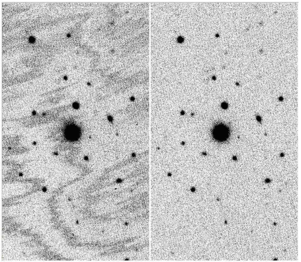
Figure 3. Example Main Survey z-band image before (left) and after (right) defringing with 10 PCs. The peak-to-peak amplitude of the fringes is up to 30 counts in this particular image, with a background level of $\sim400$
counts.
$\sim400$
counts.
2.4. Masking of electronic noise
Following a period of observatory downtime in 2015, a new source of electronic noise became apparent in the raw images. With correlated fluctuations across all amplifiers, amplitudes of tens to hundreds of counts, typically spanning three pixels in the x direction, and small positional differences between the four quadrants of the mosaic related to timing offsets during the readout process, the source of this noise was subsequently identified as due to ground loops being introduced to the electronics. The problem was rectified by cabling modifications on 2018 July 25.
For DR2 images obtained after November 2015, the following procedure was applied to identify and flag the affected pixels in the associated mask file: after flat-field correction and immediately prior to the flagging of cosmic rays, and taking each mosaic quadrant in turn, the astrophysical sources were masked, based on a 2 $\sigma$
detection threshold in SOURCE EXTRACTOR. We also masked the pixels previously flagged by the SDP (bad pixels, saturated pixels, pixels affected by cross-talk, etc.). The data from the 16 amplifiers (eight CCDs) of the quadrant were appropriately flipped to align pixels read out at the same instant, and the minimum unmasked value at each pixel location was used to construct a source-free image. After subtracting the overall median count value of the source-free image to remove the background, pixels with values exceeding 7
$\sigma$
detection threshold in SOURCE EXTRACTOR. We also masked the pixels previously flagged by the SDP (bad pixels, saturated pixels, pixels affected by cross-talk, etc.). The data from the 16 amplifiers (eight CCDs) of the quadrant were appropriately flipped to align pixels read out at the same instant, and the minimum unmasked value at each pixel location was used to construct a source-free image. After subtracting the overall median count value of the source-free image to remove the background, pixels with values exceeding 7 $\sigma$
in either direction were flagged, as was one pixel to the left and one to the right of the outlying pixel. The flagged pixels were assigned values of 64 in the image mask (see Figure 4 for an example).
$\sigma$
in either direction were flagged, as was one pixel to the left and one to the right of the outlying pixel. The flagged pixels were assigned values of 64 in the image mask (see Figure 4 for an example).
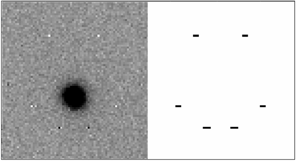
Figure 4. Example of electronic noise near the centre of a CCD, showing the near-symmetric behaviour in the two amplifiers used to read out each detector (left), and the resulting image mask (right) with the affected pixels flagged by the procedure described in Section 2.4.
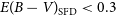
2.5. Photometric zero-point calibration
For DR1, we used the American Association of Variable Star Observers (AAVSO) Photometric All Sky Survey (APASS DR9; Henden et al. Reference Henden, Templeton, Terrell, Smith, Levine and Welch2016) and 2MASS catalogues as the external reference points for photometric calibration, after training a transformation from APASS to Pan-STARRS1 (PS1) bandpasses using stars in a common area and then applying a theoretical colour transformation from PS1 to SkyMapper bandpasses based on stellar templates. We subsequently noted significant inhomogeneities in the APASS zero points across the sky, but now that Gaia DR2 provides all-sky homogeneity, we anchor the SkyMapper DR2 zero points to that.
In the Asteroid Terrestrial-impact Last Alert System (ATLAS) Reference Catalog 2 (Refcat2), Tonry et al. (Reference Tonry, Denneau and Flewelling2018) present a transformation from the Gaia filters Bp and Rp to PS1 griz, including a correction based on the flux density of neighbouring stars. This was capable of predicting PS1 griz magnitudes all over the sky to within less than 0.01 mag RMS. We then apply an updated PS1-to-SkyMapper bandpass transformation, using a restricted set of calibrator stars and an updated dust term. The bandpass transformation is derived from synthetic photometry using the stellar spectral library of Pickles (Reference Pickles1998).
In the case of the uv filters, this process involves extrapolation from the PS1 g-band, which has a strong colour term (see below) and is thus prone to significant error propagation. Since we do not have prior knowledge of the metallicity of our zero-point stars, we ignore the significant metallicity dependence in this transformation, which increases zero-point scatter due to metallicity scatter among the calibrator stars, and potentially introduces a subtle calibration drift due to stellar-population gradients across the sky.
Stars are only used as calibrator stars when (i) Gaia DR2 reports a parallax of $>\!1$
milliarcsec, meaning the stars are closer than 1 kpc, to limit the potential impact of dust extinction, (ii) Gaia photometry is considered reliable and not a blend of sources, and (iii) the star is in a suitable colour range for linear colour terms; for details, see Tonry et al. (Reference Tonry, Denneau and Flewelling2018). We further require that either the integrated
$>\!1$
milliarcsec, meaning the stars are closer than 1 kpc, to limit the potential impact of dust extinction, (ii) Gaia photometry is considered reliable and not a blend of sources, and (iii) the star is in a suitable colour range for linear colour terms; for details, see Tonry et al. (Reference Tonry, Denneau and Flewelling2018). We further require that either the integrated $E(B-V)$
reddening in the all-sky map of Schlegel, Finkbeiner, & Davis (Reference Schlegel, Finkbeiner and Davis1998), hereafter SFD is below 0.3 mag or the star has a meaningful (i.e., non-zero) value for the
$E(B-V)$
reddening in the all-sky map of Schlegel, Finkbeiner, & Davis (Reference Schlegel, Finkbeiner and Davis1998), hereafter SFD is below 0.3 mag or the star has a meaningful (i.e., non-zero) value for the $A_G$
extinction estimated in Gaia DR2.
$A_G$
extinction estimated in Gaia DR2.
We estimate extinction levels for sight lines with $E(B-V)_{\rm SFD}<0.3$
using
$E(B-V)_{\rm SFD}<0.3$
using $A_V = 0.86 \times 3.1 E(B-V)$
(Schlafly & Finkbeiner Reference Schlafly and Finkbeiner2011), while reducing the estimated
$A_V = 0.86 \times 3.1 E(B-V)$
(Schlafly & Finkbeiner Reference Schlafly and Finkbeiner2011), while reducing the estimated $A_V$
further at higher SFD dust levels to take into account that the stars are most likely not reddened by the full dust column. To this end, we use the Gaia reddening estimate
$A_V$
further at higher SFD dust levels to take into account that the stars are most likely not reddened by the full dust column. To this end, we use the Gaia reddening estimate $A_G$
, but we do not simply adopt it owing to its large noise. Instead, we determine a weighted average between the SFD estimate and the Gaia estimate, whereby the fractional SFD weight declines from 1 at
$A_G$
, but we do not simply adopt it owing to its large noise. Instead, we determine a weighted average between the SFD estimate and the Gaia estimate, whereby the fractional SFD weight declines from 1 at $E(B-V)_{\rm SFD}=0.3$
towards zero for extremely high
$E(B-V)_{\rm SFD}=0.3$
towards zero for extremely high $E(B-V)_{\rm SFD}$
values. Our final bandpass transformations are then (subscript to u-band denotes airmass, over which we interpolate when applying to a given image) as follows:
$E(B-V)_{\rm SFD}$
values. Our final bandpass transformations are then (subscript to u-band denotes airmass, over which we interpolate when applying to a given image) as follows:
 $$
\begin{align*}
u_2 & = g_{\rm PS} + 0.783 + 1.127(g-i) - 0.313\times A_V, \\[2pt]
u_1 & = g_{\rm PS} + 0.778 + 1.350(g-i) - 0.354\times A_V, \\[2pt]
v & = g_{\rm PS} + 0.333 + 1.495(g-i) - 0.459\times A_V, \\[2pt]
g & = g_{\rm PS} - 0.012 - 0.174(g-i) + 0.022\times A_V, \\[2pt]
r & = r_{\rm PS} + 0.000 + 0.022(g-i) - 0.004\times A_V, \\[2pt]
i & = i_{\rm PS} + 0.011 - 0.043(g-i) - 0.007\times A_V, \\[2pt]
z & = z_{\rm PS} + 0.016 - 0.043(g-i) - 0.019\times A_V ~.
\end{align*}
$$
$$
\begin{align*}
u_2 & = g_{\rm PS} + 0.783 + 1.127(g-i) - 0.313\times A_V, \\[2pt]
u_1 & = g_{\rm PS} + 0.778 + 1.350(g-i) - 0.354\times A_V, \\[2pt]
v & = g_{\rm PS} + 0.333 + 1.495(g-i) - 0.459\times A_V, \\[2pt]
g & = g_{\rm PS} - 0.012 - 0.174(g-i) + 0.022\times A_V, \\[2pt]
r & = r_{\rm PS} + 0.000 + 0.022(g-i) - 0.004\times A_V, \\[2pt]
i & = i_{\rm PS} + 0.011 - 0.043(g-i) - 0.007\times A_V, \\[2pt]
z & = z_{\rm PS} + 0.016 - 0.043(g-i) - 0.019\times A_V ~.
\end{align*}
$$
For each SkyMapper image, we match as many stars to the zero-point catalogue as possible, and fit a two-dimensional plane to the zero-point values across the mosaic. The resulting zero-point plane is then applied to all photometry across the image.
Currently, the flat-field process includes no correction for scattered light in the twilight flats, which will be introduced in the future. Heavily dithered observations of the SkyMapper standard star fields indicate that corrections are mostly less than 2% in sensitivity, but in the 1% area of the mosaic that is closest to the corners the calibration offsets can reach locally up to 5%. This means that an object measured once in a very corner of the mosaic and another time in the inner bulk area could show apparent variability up to a 5% level in extreme cases.
2.6. Distil process for master table
The final step in the production of the data release is a distil process. It uses the photometry table that has one row per detection and creates a master table with one row per unique astrophysical object. When objects have multiple detections in the same filter, these may be from both the Shallow Survey and the Main Survey, and they are combined into best-estimate values assuming the object is not variable. Variable sources are of course better characterised by their individual detections in the photometry table, as sampled by the observed cadence. (The timescales for and between visits were described in Section 2.1.)
2.6.1. Flagging and combining detections
We retain any FLAGS values assigned by Source Extractor (up to bit 7, value 128) in the photometry table, but can also add several possible values from our post-processing (values 512, 1 024, 2 048, and 4 096):
1. As in DR1, we set bit value 512 for very faint detections that we consider dubious and a potential source of error. This includes all sources on Shallow Survey images that have any one of four crucial magnitudes fainter than 19 mag or NULL: the PSF magnitude, the Petrosian magnitude (Petrosian Reference Petrosian1976), the 15 arcsec aperture magnitude, and the 5 arcsec aperture magnitude (after applying the aperture correction). Sources on the deeper Main Survey images are flagged when any of the PSF, Petrosian, or 5 arcsec aperture magnitude is NULL, or when the error on the 5 arcsec aperture magnitude is greater than 0.3 mag. This treatment makes sure that very faint detections in the Shallow Survey are ignored for the benefit of letting the Main Survey alone define their distilled properties, while faint Main Survey-only detections are included into the master table.
2. We set bit value 1 024 for sources whose light profile appears significantly more concentrated than a PSF, using the selection rule MAG_APC02 minus;MAG_APR15
$<-1$
AND CHI2_PSF
$>10$
; this is unchanged from DR1.Footnote d3. We set bit value 2 048 for detections that are too close to bright stars and thus have a high chance to be affected by optical reflections. Around such stars, we flag all sources within a specific angular distance, using an algorithm improved over DR1. We now use bright stars from ATLAS Refcat2, transform their PS1 photometry to SkyMapper uvgriz magnitudes, and calculate the flagging radius around each star as
$10^{-0.2 m}$
degrees using the expected SkyMapper magnitude. For stars fainter than
$ (u,v,g,r,i,z)=(4,5,8.5,8.5,6,5) ,$
we do not seem to get bad detections and thus do not apply any flags near these. Note that reflections are not concentric around the stars, so the flagging radius has been enlarged to account for the maximum affected area across the whole field of view.4. We set bit value 4 096 for a small set of master table entries around the RA=0/360 boundary that were inadequately merged between filters.


When a detection of a source is identified by Source Extractor as saturated or affected by many masked pixels, or has been flagged with one of the rules above (criterion: FLAGS $\,>=\,$
4 OR NIMAFLAGS
$\,>=\,$
4 OR NIMAFLAGS $\,>=\,$
5), we declare it as a bad detection, and ignore it when determining master table properties for the source. When there are only bad detections for a source, then, to avoid omitting the source from the master table, we use the bad detections to populate just the position-related columns (including cross-matching with other catalogues), and the photometric columns are set to NULL. Objects without good detections in a given filter can be identified by having
$\,>=\,$
5), we declare it as a bad detection, and ignore it when determining master table properties for the source. When there are only bad detections for a source, then, to avoid omitting the source from the master table, we use the bad detections to populate just the position-related columns (including cross-matching with other catalogues), and the photometric columns are set to NULL. Objects without good detections in a given filter can be identified by having $\{\rm F\}\_{\rm NGOOD}\,=\,0$
, where {F} is the filter name; and if no filters have good detections, then
$\{\rm F\}\_{\rm NGOOD}\,=\,0$
, where {F} is the filter name; and if no filters have good detections, then $\text{NGOOD}\,=\,0$
.
$\text{NGOOD}\,=\,0$
.
We follow the same approach as in DR1 to merge individual detections into parent objects, first within a filter, and then among the filters. Sometimes this process creates parent objects with multiple child objects and we treat them as described below. We acknowledge that this process is intrinsically problematic, and hope to improve it for the next data release.
When merging individual detections for one filter, some point sources on some images are split into two child objects due to suboptimal settings in SOURCE EXTRACTOR. In DR1, we added their fluxes in the distil process, but as we have more observations per source in DR2, we chose to remove such detections from the photometry table and use only the others. We note that we lose an object entirely in a filter when it has multiple children in all images of that filter. This also happens to genuine binary stars when they are merged into a single object by the process. Unfortunately, in DR2 this data cannot be recovered from the provided tables.
When merging the six filters, we encounter situations (as in DR1) where a global object ID is associated with two detections in some of the filters. We then leave out the (likely unphysical) results for those filters from the master table. However, data for an omitted filter can still be found in the photometry table.
2.6.2. Combining measurements into distilled values
How we combine individual measurements depends on the nature of the measurement:
1. For RA/Dec positions and the observing epoch, we determine simple averages and standard deviations of all values; the Petrosian radius, selected only from the r-band measurements, is also averaged.
2. For FLUX_MAX and CLASS_STAR, we pick the highest value; FLAGS are bitwise OR-combined, and NIMAFLAGS values are summed up.
3. PSF and Petrosian magnitudes are combined with a more complex algorithm: first, we determine more realistic errors of our individual measurement values by quadratically adding floors of 0.01 mag to reflect flat-field uncertainties (consistent across all filters); then we use the set of PSF magnitudes to identify outlier measurements: we calculate an inverse variance-weighted median magnitude from the list of values; next we obtain their median absolute deviation (MAD) from the weighted median; and then we clip possible outlier measurements from the list when they deviate from the weighted median value by
$>\!3\times$
the larger of the MAD and their individual error. In a final step, we combine the remaining values into an inverse variance-weighted measurement of the mean magnitude and its final error, using the same list of detections for both the PSF and the Petrosian magnitude. The photometry table contains a column USE_IN_CLIPPED that identifies the measurements used for the mean. As a variability indicator, we also determine a reduced
$\chi^2$
from the full set of PSF magnitudes and store it in column {F}_RCHI2VAR, where {F} is the filter name.


Objects that are saturated or have bad flags in all available frames will only have moderately useful information. Several columns are filled with NULL values on purpose, but positions are still averaged and FLAGS are still OR-combined. They can be easily identified by their FLAGS value in the master table ( $\ge 4$
).
$\ge 4$
).
2.6.3. Cross-matched external catalogues
As in DR1, we cross-match the master table with several external catalogues. For large photometric catalogues, we determine the matching external object and record its ID and projected distance within the master table. For small catalogues (mostly spectroscopic), we match in reverse direction and record the SkyMapper object and distance in the external catalogue as DR2_ID and DR2_DIST. The maximum distance for all cross-matches is 15 arcsec, motivated by the region in which our 1D PSF magnitudes may be affected.
The cross-matched large catalogues include 2MASS Point Source Catalog (PSC) (Skrutskie et al. Reference Skrutskie, Cutri and Stiening2006), AllWISE (Wright et al. Reference Wright, Eisenhardt and Mainzer2010; Mainzer et al. Reference Mainzer2011), ATLAS Refcat2 (Tonry et al. Reference Tonry, Denneau and Flewelling2018), Gaia DR2 (Gaia Collaboration et al. Reference Brown and Vallenari2018), the Revised Catalog of GALEX Ultraviolet Sources (GUVcat; Bianchi, Shiao, & Thilker Reference Bianchi, Shiao and Thilker2017), PS1 DR1 (Chambers et al. Reference Chambers2016; Magnier et al. Reference Magnier2016), SkyMapper DR1 (Wolf et al. Reference Wolf, Onken and Luvaul2018a), and UCAC4 (Zacharias et al. Reference Zacharias, Finch, Girard, Henden, Bartlett, Monet and Zacharias2013). In the case of Gaia, we record the two nearest matches, which helps with identifying blended sources. The master table is also cross-matched against itself to identify the ID and distance to the nearest neighbour of every source (up to 15 arcsec).
The reverse-cross-matched catalogues include the 2dF Galaxy Redshift Survey (2dFGRS; Colless et al. Reference Colless2001), the 2dF QSO Redshift Survey (2qz6qz; Croom et al. Reference Croom, Smith, Boyle, Shanks, Miller, Outram and Loaring2004), the 2dFLenS Survey (Blake Reference Blake, Amon and Childress2016), the 2MASS Redshift Survey (2MRS; Huchra et al. Reference Huchra, Macri and Masters2012), the 6dF Galaxy Survey (6dFGS; Jones et al. Reference Jones2004; Jones et al. Reference Jones2009), the GALAH survey DR2.1 (Buder et al. Reference Buder, Asplund and Duong2018), MILLIQUAS v6.2b (Flesch Reference Flesch2015), the Hamburg/ESO Survey for Bright QSOs (HES QSOs; Wisotzki et al. Reference Wisotzki, Christlieb, Bade, Beckmann, Köhler, Vanelle and Reimers2000), and the AAVSO International Variable Star Index (VSX; Watson, Henden, & Price Reference Watson, Henden and Price2006; Watson et al. Reference Watson, Henden and Price2017). When using cross-matched IDs, care needs to be taken to observe the distance column in order to only select detections that are likely to be physically associated.
3. DR2 properties
3.1. Image data set
Data Release 2 contains a total of 121 494 exposures, comprised of 84 946 exposures from the Shallow Survey that provide nearly full hemispheric coverage in all filters with multiple visits, and 36 548 exposures from the Main Survey providing partial coverage in terms of fields, filters, and depth (Table 1). A total of $\sim\!3.7$
millionPlease spell out at ‘FITS’ first use, if needed. individual CCDs passed the quality cuts. The median airmass is 1.11, but a tail to airmass 2 is unavoidable given that the survey footprint includes the South Celestial Pole.
$\sim\!3.7$
millionPlease spell out at ‘FITS’ first use, if needed. individual CCDs passed the quality cuts. The median airmass is 1.11, but a tail to airmass 2 is unavoidable given that the survey footprint includes the South Celestial Pole.
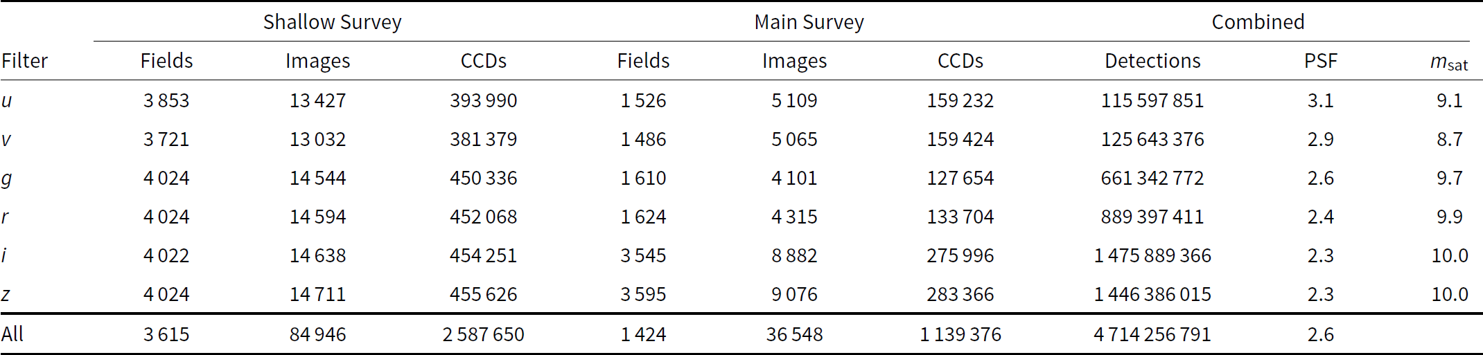
Table 1. DR2 image numbers by filter and survey segment. The row All refers to the sum for the Images, CCDs, and Detections columns, but for the Fields column refers to the distinct number that have coverage in all filters. PSF represents the median FWHM in arcsec. The saturation limit in the last column is the median value, but ranges over more than $\pm 1$
mag within each filter due to variable observing conditions.
$\pm 1$
mag within each filter due to variable observing conditions.
As in DR1, the median FWHM of the PSF among all DR2 images ranges from 2.3 arcsec in z-band to 3.1 arcsec in u-band (see Figure 5). Although the median is similar in the two survey components, the distribution is broader in the Shallow Survey: it benefits from occasional short ( $<\!20$
s) periods of good seeing, but it also includes observations in bad seeing, when the image scheduling software (‘the scheduler’) avoids the Main Survey and defaults to the Shallow Survey. The median elongation is independent of filter, with values of 1.12 and 1.14 in the Shallow and Main Survey, respectively.
$<\!20$
s) periods of good seeing, but it also includes observations in bad seeing, when the image scheduling software (‘the scheduler’) avoids the Main Survey and defaults to the Shallow Survey. The median elongation is independent of filter, with values of 1.12 and 1.14 in the Shallow and Main Survey, respectively.
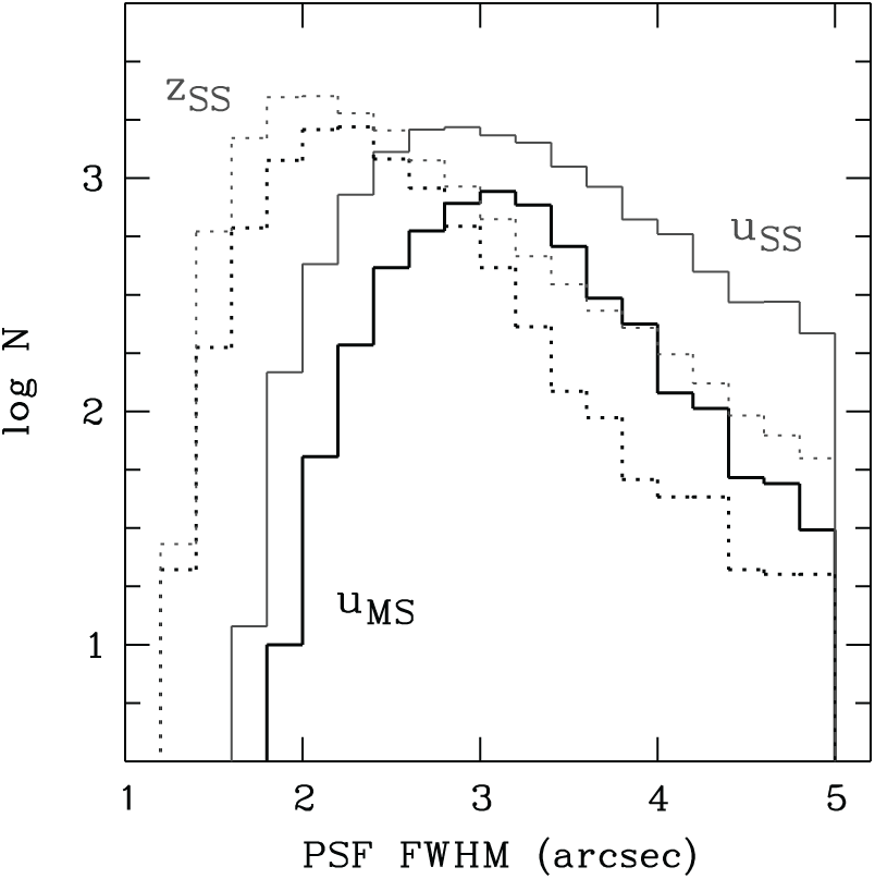
Figure 5. Distribution of PSF FWHM in DR2 images: u-band images (solid lines) have a median seeing of 3.1 arcsec seeing compared to 2.3 arcsec in z-band (dotted lines). The Main Survey (black lines) has a tighter distribution than the Shallow Survey (grey lines).
Most images of the Shallow Survey are read-noise limited, as the median sky background is less than 100 counts, except for the z-band images that are mostly background-limited. Median count levels in the Shallow Survey have slightly increased in DR2 as most of the frames added since DR1 were taken in full-moon conditions. In the Main Survey, 98% of uv frames are read-noise limited because the Main Survey colour sequence is not observed in bright time, and so the median background is 11 counts. The griz frames, in contrast, are all background-limited in the Main Survey, with sky levels always above 100 counts and median levels range from 227 in g-band to 646 in z-band.
The photometric zero points show long-term drifts towards lower efficiencies across all filters due to dust settling on the telescope optics over time (see Figure 6). A cleaning of the telescope optics on 2015 May 5 (Modified Julian Date, MJD, 57147) improved the zero points by $\sim\!0.3$
mag, as did another cleaning on 2018 February 1 (MJD 58150). We observe an average trend in the loss of system throughput on the order of 1% per month, which might motivate an annual cleaning in the future. Most zero points for a given filter scatter within 0.1 mag RMS at a given calendar epoch, but some nights with bad weather produce tails with higher atmospheric extinction.
$\sim\!0.3$
mag, as did another cleaning on 2018 February 1 (MJD 58150). We observe an average trend in the loss of system throughput on the order of 1% per month, which might motivate an annual cleaning in the future. Most zero points for a given filter scatter within 0.1 mag RMS at a given calendar epoch, but some nights with bad weather produce tails with higher atmospheric extinction.
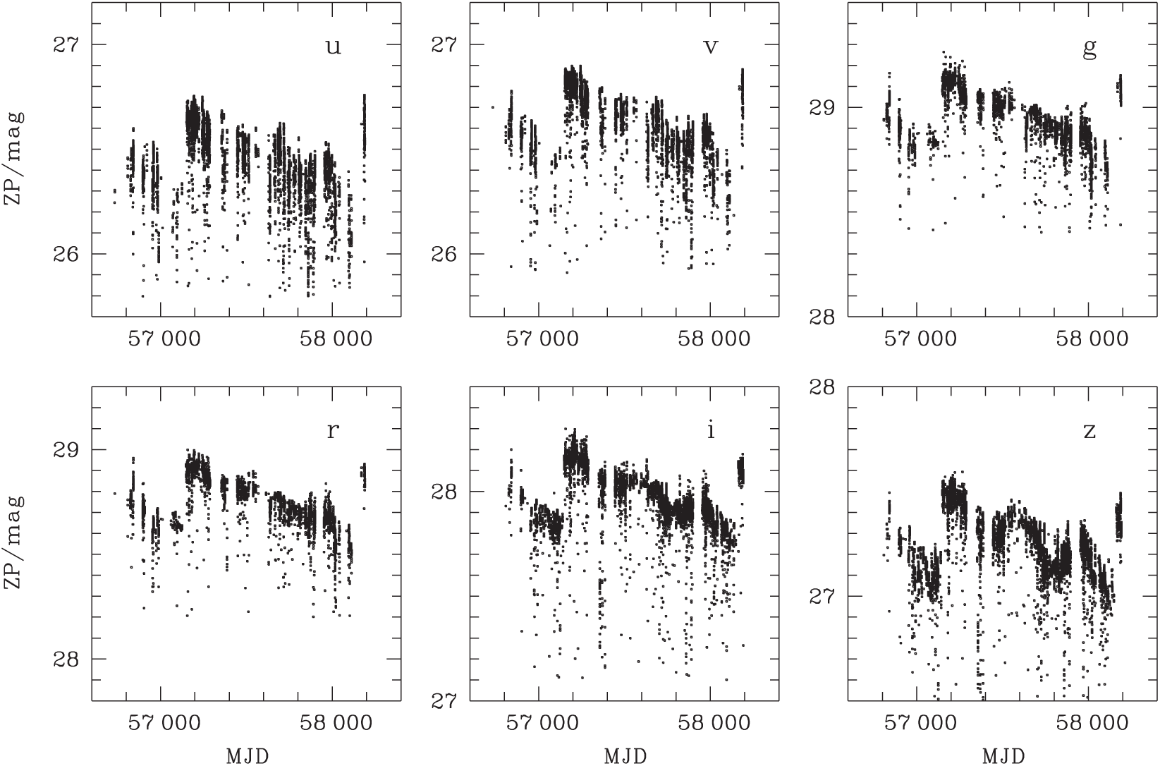
Figure 6. Time evolution of magnitude zero points per filter for Main Survey exposures: the gradient shows gradual deterioration of optical reflectivity at a mean rate of $-0.33$
mmag d-1. Cleaning of the telescope optics on 2015 May 5 (MJD 57147) and 2018 February 1 (MJD 58150) improved the zero points by
$-0.33$
mmag d-1. Cleaning of the telescope optics on 2015 May 5 (MJD 57147) and 2018 February 1 (MJD 58150) improved the zero points by $\sim\!0.3$
mag each time.
$\sim\!0.3$
mag each time.
An important influence on zero points is airmass-dependent atmospheric extinction. The SkyMapper scheduler attempts to observe any field close to meridian, but for fields with near-polar declination that still means high airmass. This effect translates into a declination-dependent upper envelope for the zero points, where fields around $-30^\circ$
enjoy best transparency, while zero points deteriorate towards the South Celestial pole (see Figure 7). The effect is most pronounced in u-band (which even changes its filter curve due to the atmospheric cut-off), where we lose over 0.7 mag between zenithal declinations and the pole.
$-30^\circ$
enjoy best transparency, while zero points deteriorate towards the South Celestial pole (see Figure 7). The effect is most pronounced in u-band (which even changes its filter curve due to the atmospheric cut-off), where we lose over 0.7 mag between zenithal declinations and the pole.
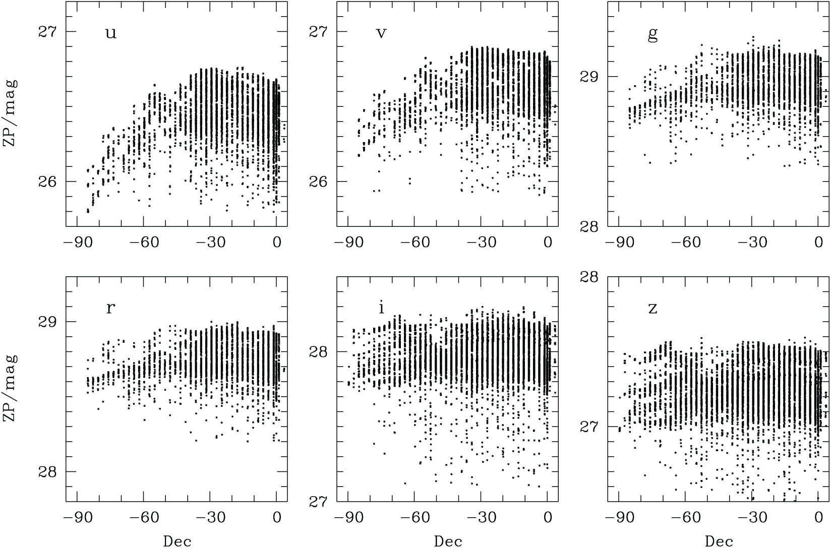
Figure 7. Declination dependence of Main Survey zero points: the upper envelope results from airmass-dependent atmospheric throughput. The u-band suffers $>\!0.75$
mag loss from zenith to the Celestial pole. While the SkyMapper scheduler attempts to observe at minimal airmass, near-polar fields never rise to low airmass.
$>\!0.75$
mag loss from zenith to the Celestial pole. While the SkyMapper scheduler attempts to observe at minimal airmass, near-polar fields never rise to low airmass.
3.2. Sky coverage
The mixture of Shallow Survey and Main Survey data and their sky coverage can be seen from Figure 8, which shows, for each filter, the deepest photometric zero point for each SkyMapper field. While the zero-point maps distinguish between the areas with Shallow Survey (light) and Main Survey (dark) images, the FWHM and background levels for each observation serve to further modify the true point source sensitivity across the sky.
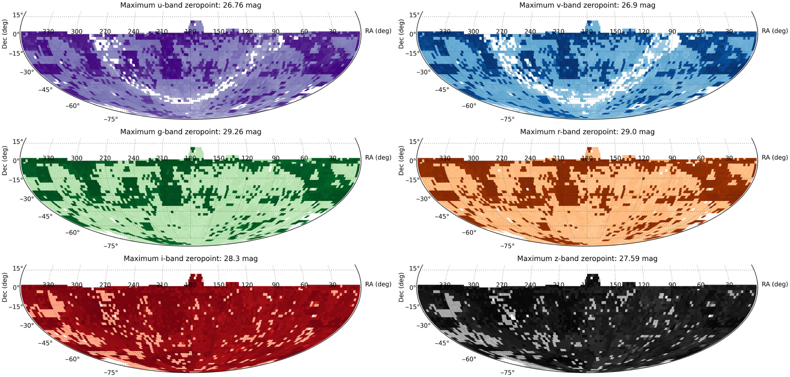
Figure 8. Maximum photometric zero points for each field, separated by filter. Darker colours indicate deeper data, with white fields having no images. The nominal zero-point difference between Shallow Survey and Main Survey is roughly given by the ratio of exposure times, amounting to (1.0, 1.75, 3.25, 3.25, 2.5, 1.75) mag in (u,v,g,r,i,z), respectively.
The sky coverage of the Main Survey falls into two filter groups owing to the observing strategy: uvgr coverage is driven by the colour sequences that are available for 40% of the hemisphere, and slight differences in image availability stem from the application of hard quality thresholds to individual images. In contrast, the iz filters cover nearly the whole hemisphere because of twilight observations that are dedicated to this filter pair.
DR2 has tighter limits on image quality than DR1, in particular for zero-point homogeneity within exposures; this means that users could find data missing in DR2 that was previously part of DR1. Since better data are not always available, some DR1 objects will be absent.
3.3. Photometric table data set
The data set comprises tables with observing information (images, ccds, and mosaic), tables of on-sky photometry, (master and photometry), and copies of external catalogues pre-matched to SkyMapper sources, so that users can quickly generate multi-wavelength table joins.
DR2 provides instantaneous photometry, i.e. measurements made on individual images, as well as averages distilled from repeat measurements, which will be meaningful for non-variable objects. Since objects are only searched on individual images and not on image stacks, the object catalogue is less deep than the data set would allow in principle.
However, the distilled photometry in the master table reduces errors by combining all individual measurements that are flagged as reliable, and the distilled errors reflect variations beyond photon noise, such as resulting from uneven throughput variations. A planned addition for the next release is searching for objects on deeper co-added frames and performing forced-position photometry, which will create a deeper catalogue and more precise photometry for extended sources.
Most science applications will be served well with data from the master table alone, which contains astrometry and six-filter PSF and Petrosian photometry, as well as flags and cross-link IDs to multi-wavelength tables from external sources. Each row in the master table represents one astrophysically unique object.
The more detailed photometry table contains one row per unique detection in any SkyMapper image. A single object from the master table may thus appear in several dozen rows in the photometry table, depending on the number of visits to the field and the number of filters in which the object is visible. Objects can be identified or joined to the master table with the OBJECT_ID column (described further in the next section).
3.3.1. Master table
The DR2 master table contains about half a billion (505 176 667) unique astrophysical objects. Their photometric measurement can have good flags (SOURCE EXTRACTOR FLAGS 0 to 3, no other issues) or bad flags (SOURCE EXTRACTOR FLAGS $\geq$
4 or other issues).
$\geq$
4 or other issues).
Among the half billion objects, about 2.75 million (0.55%) do not have a single good measurement in any filter, either because they are saturated in all filters or because they are too close to a very bright star and thus flagged to have possibly bad photometry or be bogus detections due to scattered light.
A further $\sim82.3$
million (16%) have at least one filter with only one good measurement. The remaining 422 839 424 objects (83%) have more than one good measurement in all filters in which they are detected at all. Filters without any detections do not count towards this consideration.
$\sim82.3$
million (16%) have at least one filter with only one good measurement. The remaining 422 839 424 objects (83%) have more than one good measurement in all filters in which they are detected at all. Filters without any detections do not count towards this consideration.
The astrometric calibration of DR2 is done as in DR1 and astrometric precision has not changed overall. The median offset between our positions and those in Gaia DR2 is 0.16 arcsec for all objects and 0.12 arcsec for bright, well-measured objects. In the next release, we plan to switch the astrometric reference frame to Gaia DR2.
The change in calibration procedure from DR1 to DR2 implies that every object in common between the two releases will have new photometry (and a new OBJECT_ID).Footnote e In the ugri filters, the average change among bright stars is less than 1%, while the average v-band magnitude has dimmed by 2.5%; that is, it moved by the opposite of what was suggested in Casagrande et al. (Reference Casagrande, Wolf and Mackey2019), and the average z-band magnitude has brightened by 1.5%.
Figure 9 shows a map of the magnitude differences between our two data releases, which are almost entirely a result of changing the calibration reference; the change from APASS DR9 in our DR1 to Gaia DR2 in our DR2 imports the all-sky homogeneity of Gaia into the SkyMapper calibration and removes the substructure we had imported previously from APASS DR9.
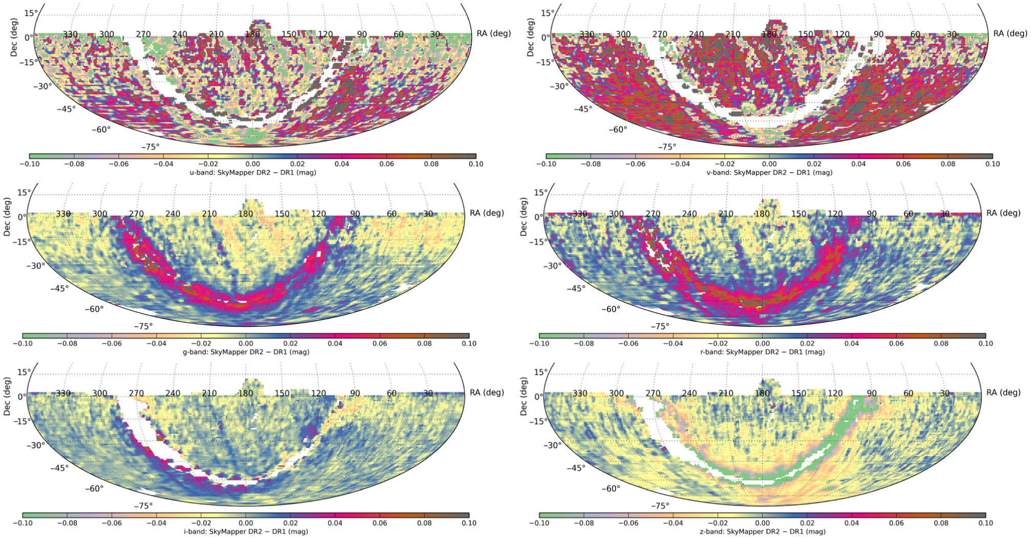
Figure 9. Comparison of DR2 photometry with DR1 photometry in all filters: plotted are the median magnitude differences per deg $^2$
, restricted to objects with PSF magnitudes brighter than 16. These differences are expected to result primarily from the improved calibration procedure in DR2.
$^2$
, restricted to objects with PSF magnitudes brighter than 16. These differences are expected to result primarily from the improved calibration procedure in DR2.
When we compare our measured photometry with that predicted from Gaia for the sample of our zero-point stars, we find on average no offset in any filter, as expected by design of our calibration procedure. We find, however, RMS dispersions among magnitude differences that range from 1.5% for g and r filters to 5% for the u-band. This is a result of true physical dispersion, presumably due to the distribution of metallicity values and their effect on measured u-band magnitudes, where the predicted magnitudes ignore metallicity and involve just a mean transformation for the overall sky population.
Figure 10 compares our measured photometry with that of Pan-STARRS1 DR1, assuming bandpass transformations by Tonry et al. (Reference Tonry, Denneau and Flewelling2018). We restrict the comparison to the magnitude range $[14.5,17.5]$
for all four filters, where both surveys should be complete and free from saturation effects. The predominant differences are close to the Galactic plane and follow Galactic structure, and so are likely due to the treatment of reddening and/or issues of source density in crowded fields (cf. Tonry et al. Reference Tonry, Denneau and Flewelling2018). The mottled effect in the (
$[14.5,17.5]$
for all four filters, where both surveys should be complete and free from saturation effects. The predominant differences are close to the Galactic plane and follow Galactic structure, and so are likely due to the treatment of reddening and/or issues of source density in crowded fields (cf. Tonry et al. Reference Tonry, Denneau and Flewelling2018). The mottled effect in the ( $g-r$
) map (which is shown at higher contrast than the others) is primarily due to residual flat-fielding imperfections in the SkyMapper images.
$g-r$
) map (which is shown at higher contrast than the others) is primarily due to residual flat-fielding imperfections in the SkyMapper images.
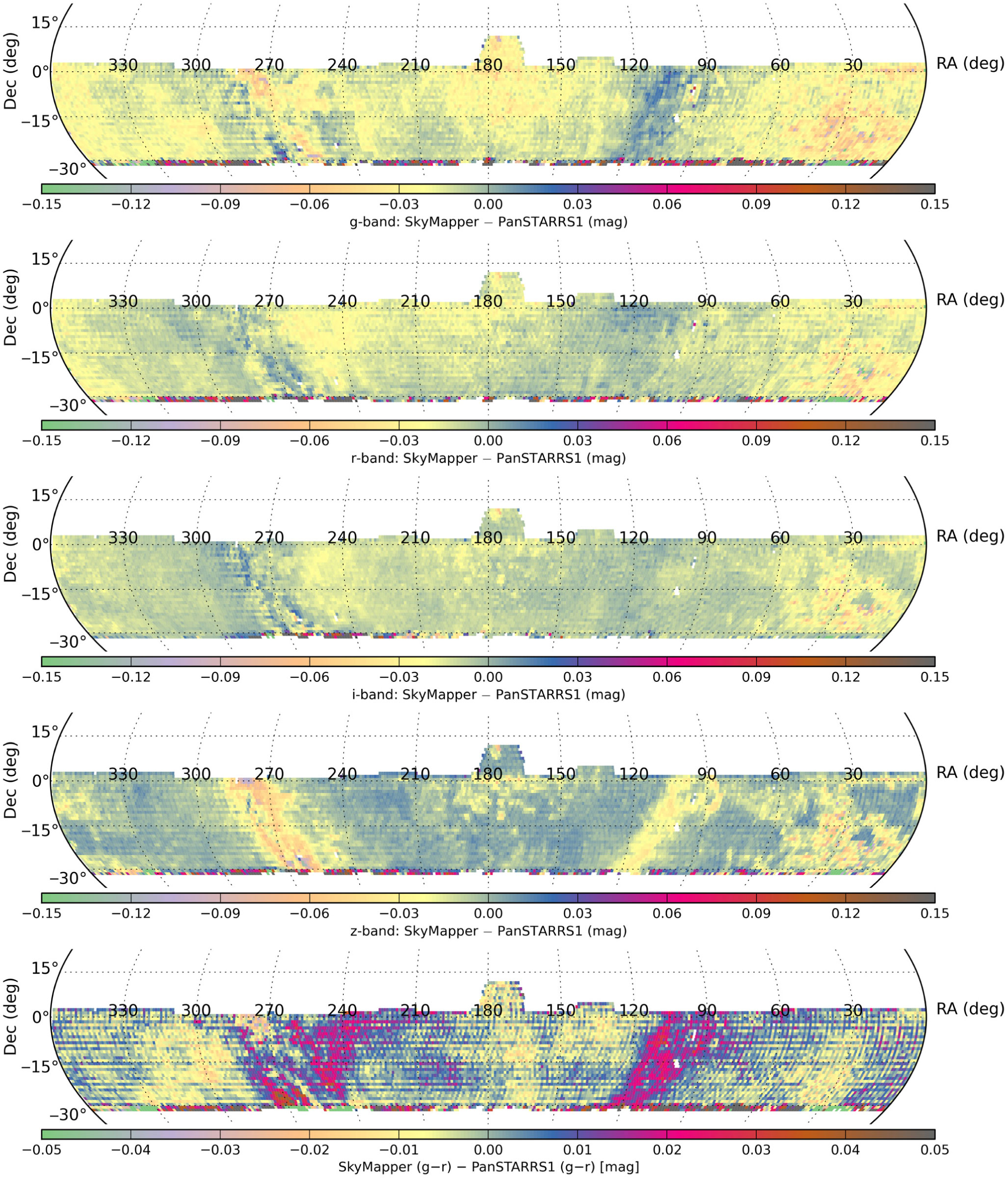
Figure 10. Comparison of SkyMapper DR2 photometry with Pan-STARRS1 DR1 photometry in g,r,i,z after applying bandpass transformations by Tonry et al. (Reference Tonry, Denneau and Flewelling2018): plotted are the median magnitude differences per deg $^2$
, restricted to objects with PSF magnitudes between 14.5 and 17.5. The large offsets at the Southern edge of the PS1 coverage are where PS1 becomes unreliable. The bottom panel compares the median
$^2$
, restricted to objects with PSF magnitudes between 14.5 and 17.5. The large offsets at the Southern edge of the PS1 coverage are where PS1 becomes unreliable. The bottom panel compares the median $g-r$
colours in a high-contrast map and shows that the most extreme differences reach
$g-r$
colours in a high-contrast map and shows that the most extreme differences reach $\pm 0.03$
mag.
$\pm 0.03$
mag.
We also see small-scale structure away from the plane, where star densities should be generally low. Focusing on a small halo region around RA $\,=180$
, we find RMS differences in the map of less than 0.01 mag in gr filters and also in the
$\,=180$
, we find RMS differences in the map of less than 0.01 mag in gr filters and also in the $g-r$
colour map, although peak-to-peak the
$g-r$
colour map, although peak-to-peak the $g-r$
colour can range by 0.035 mag in the halo fields at Northern Galactic latitudes.
$g-r$
colour can range by 0.035 mag in the halo fields at Northern Galactic latitudes.
We estimate the internal reproducibility of DR2 photometry from repeat measurements of bright stars with good flags and find RMS values in the PSF magnitude of 10 mmag in u and v filter, and 7 mmag in griz.
We also show a map of the median colours of stars as measured by SkyMapper and PS1 ( $g-r$
) as well as Gaia (
$g-r$
) as well as Gaia ( $B_p-R_p$
) in Figure 11. We note that the visible structures are extremely similar. Overall, we see the well-known trend with Galactic latitude: halo fields are dominated by red stars seen through little reddening by interstellar dust, while intermediate-latitude fields are populated increasingly by younger and bluer stars; closer to the Galactic plane dust reddening makes the population appear strongly redder, while some special regions on the plane show only unreddened foreground stars, as the most highly reddened stars are invisible.
$B_p-R_p$
) in Figure 11. We note that the visible structures are extremely similar. Overall, we see the well-known trend with Galactic latitude: halo fields are dominated by red stars seen through little reddening by interstellar dust, while intermediate-latitude fields are populated increasingly by younger and bluer stars; closer to the Galactic plane dust reddening makes the population appear strongly redder, while some special regions on the plane show only unreddened foreground stars, as the most highly reddened stars are invisible.
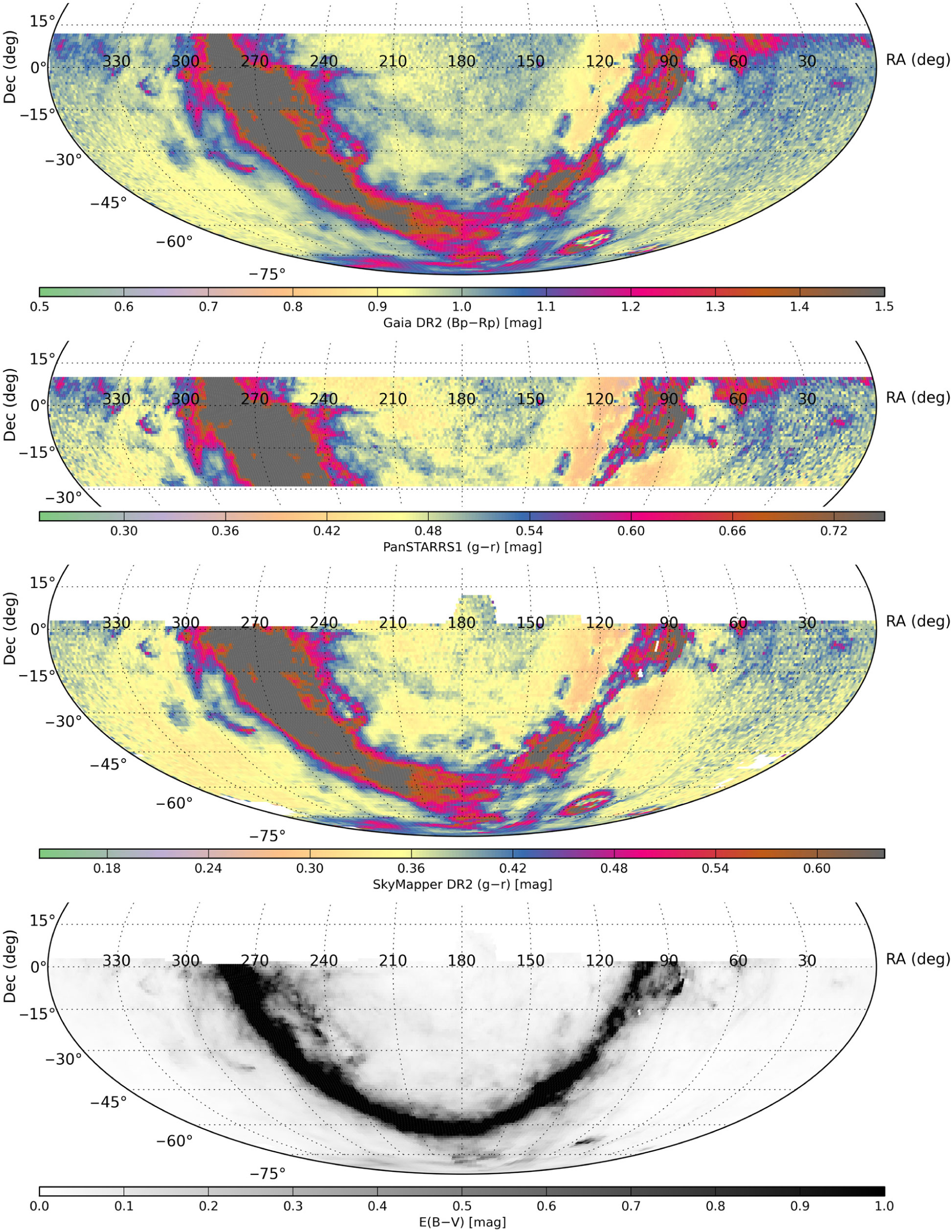
Figure 11. Median colour of the stellar population as seen in Gaia $B_p-R_p$
, Pan-STARRS1
$B_p-R_p$
, Pan-STARRS1 $g-r$
and SkyMapper
$g-r$
and SkyMapper $g-r$
: plotted are the median colours per deg
$g-r$
: plotted are the median colours per deg $^2$
, restricted to objects with magnitudes 14.5 to 17.5. The bottom panel shows the median
$^2$
, restricted to objects with magnitudes 14.5 to 17.5. The bottom panel shows the median $E(B-V)$
reddening value from Schlegel et al. (Reference Schlegel, Finkbeiner and Davis1998).
$E(B-V)$
reddening value from Schlegel et al. (Reference Schlegel, Finkbeiner and Davis1998).
Finally, Figure 12 shows the number counts from the master table in all six passbands using only objects with PSF magnitude errors of less than 5%, corresponding to $>\!20\sigma$
-detections. The curve for each filter shows a double-peaked structure as a result of combining two contributions: the Shallow Survey peaks around 17–18 mag and covers nearly the whole hemisphere, while the deeper Main Survey peaks around 19–20 mag depending on filter but covers a smaller area. In the i and z filters, the double peak is not pronounced because the exposure advantage of the Main Survey translates only into a square-root gain in depth with the sky-limited background in these two filters. Generally, the peaks are softened by a range in sky transparencies and seeing levels mixed in the overall data set.
$>\!20\sigma$
-detections. The curve for each filter shows a double-peaked structure as a result of combining two contributions: the Shallow Survey peaks around 17–18 mag and covers nearly the whole hemisphere, while the deeper Main Survey peaks around 19–20 mag depending on filter but covers a smaller area. In the i and z filters, the double peak is not pronounced because the exposure advantage of the Main Survey translates only into a square-root gain in depth with the sky-limited background in these two filters. Generally, the peaks are softened by a range in sky transparencies and seeing levels mixed in the overall data set.
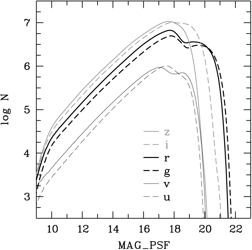
Figure 12. Number of counts per filter, restricted to objects with $<\!5$
% error in PSF magnitude. All filters show the sum of two contributions: a large area covered by the Shallow Survey that is complete to nearly 18 mag, and a smaller area covered by the Main Survey that provides deeper data and creates a second maximum.
$<\!5$
% error in PSF magnitude. All filters show the sum of two contributions: a large area covered by the Shallow Survey that is complete to nearly 18 mag, and a smaller area covered by the Main Survey that provides deeper data and creates a second maximum.
3.3.2. Photometry table
The photometry table serves three purposes that go beyond the role of the master table:
1. It lists photometry in 10 nested apertures ranging from 2 to 30 arcsec diameter. Since aperture magnitudes are seeing-dependent, and seeing changes between exposures, we do not distil these quantities.
2. It lists astrometry and photometry for individual exposures of the object. This can be used to study variability in brightness as well as motions (for examples, see Sections 3.6 and 3.7).
3. It lists photometry that is flagged as potentially (but not necessarily) bad and thus excluded from the results in the master table. Users may find the measurements useful, and the measurements may at times be correct.
Nested-aperture photometry is illustrated in Figure 13 for an extended galaxy as well as for a point source. Crucially, we report the aperture data for counts and magnitudes differently: aperture counts are listed as measured and thus represent a raw growth curve; aperture magnitudes, in contrast, are estimates of total magnitude corrected with the local growth curve (MAG_APCnn, ‘C’ indicating corrected values for an aperture diameter of nn arcsec) for all apertures smaller than 15 arcsec. The growth curve is determined by comparing the ratio of the smaller aperture flux to the 15 arcsec-aperture flux. We do this on a CCD-by-CCD basis, and the fit is allowed to vary linearly in (x, y) position on the CCD. We choose the 15 arcsec aperture as a total-magnitude reference for point source calibration; this magnitude, as well as that from the two larger apertures with diameters of 20 and 30 arcsec, is listed as measured without correction (MAG_APRnn, ‘R’ indicating raw values). PSF magnitudes are estimated as a constant-value fit to the inverse variance-weighted sequence of corrected aperture magnitudes. Formally, these fits produce estimates of PSF magnitude that appear precise to a milli-mag-level, while residual calibration errors can be much larger. Figure 13 also describes the wings of the SkyMapper PSF and shows that point sources still have a few percentage of their flux outside a 15 arcsec aperture in median seeing.
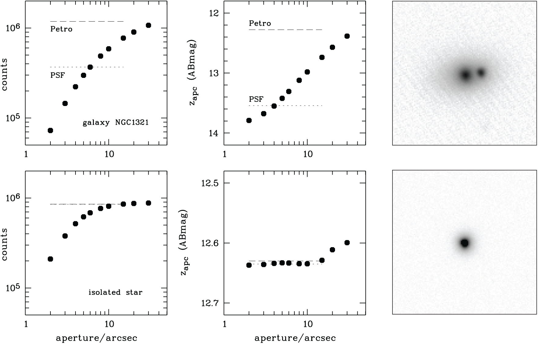
Figure 13. Growth curves of aperture measurements in the photometry table for the double source NGC 1321 (OBJECT_ID 21671053, a galaxy with a foreground star) and for a star (OBJECT_ID 21670913) in the same image (z-band, FWHM 2.7 arcsec). Left: Count rates measured in apertures with diameters of 2, 3, 4, 5, 6, 8, 10, 15, 20, and 30 arcsec (table columns FLUX_AP02 to FLUX_AP30). Overplotted are measured Petrosian and estimated 1D-PSF fluxes, which are identical within 0.5% for the star, while (unsurprisingly) the PSF flux of the galaxy is just a fraction of the total flux. Centre: Aperture magnitudes for apertures from 2 to 10 arcsec (MAG_APC02 to MAG_APC10) are corrected for the growth curve of the expected PSF at the object location assuming that a 15 arcsec aperture represents total magnitude. Aperture magnitudes for 15 arcsec (MAG_APR15) to 30 arcsec (MAG_APR30) are as measured. For the star, the various nested apertures predict nearly identical PSF magnitudes after correction, and the scatter among them is $\sim\!2$
mmag; however, the uncorrected magnitudes in the larger apertures show that there is an additional
$\sim\!2$
mmag; however, the uncorrected magnitudes in the larger apertures show that there is an additional $\sim3.5$
% of flux in the wings of the PSF between the 15 arcsec and the 30 arcsec aperture. Right: Image cut-outs of the two objects, size
$\sim3.5$
% of flux in the wings of the PSF between the 15 arcsec and the 30 arcsec aperture. Right: Image cut-outs of the two objects, size $1 \times 1$
arcmin.
$1 \times 1$
arcmin.
3.4. Limitations of PSF magnitudes
Our PSF magnitudes are based on one-dimensional (1D) growth curves of point-source light profiles over a 15 arcsec diameter, as in DR1. We estimate the precision of these growth curves from the internal reproducibility of the PSF photometry among repeat visits of the same bright objects, and find RMS variations of the PSF flux of 0.7%. However, our 1D PSF magnitudes are affected by close neighbours as a function of separation d and magnitude difference $\Delta m$
; see Figure 14. As a rule of thumb, the PSF magnitudes can be biased brighter by
$\Delta m$
; see Figure 14. As a rule of thumb, the PSF magnitudes can be biased brighter by $>\!1$
% when
$>\!1$
% when $d (\text{arcsec}) < 5 + 2 \times \Delta m$
. Binary stars of equal brightness only affect each other by
$d (\text{arcsec}) < 5 + 2 \times \Delta m$
. Binary stars of equal brightness only affect each other by $>\!1$
% if they are closer than 5 arcsec. Faint sources with bright neighbours, however, can be more strongly affected, even at 15 arcsec separation when the neighbour is over 5 mag brighter.
$>\!1$
% if they are closer than 5 arcsec. Faint sources with bright neighbours, however, can be more strongly affected, even at 15 arcsec separation when the neighbour is over 5 mag brighter.
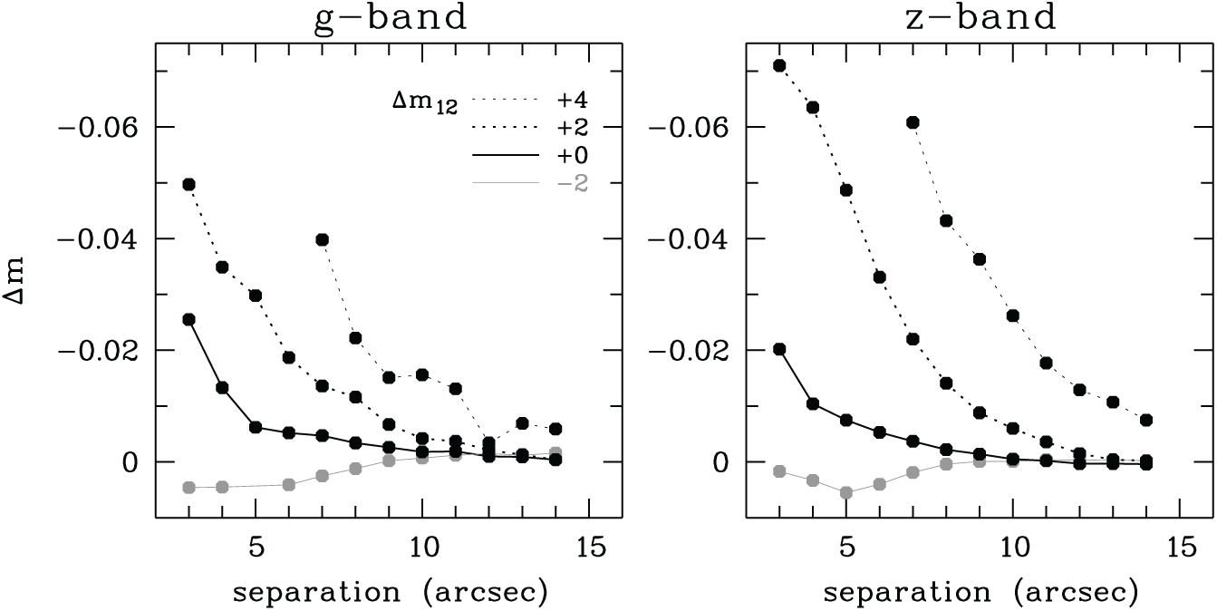
Figure 14. Effect of close neighbours on the 1D PSF magnitude of stars: flux from neighbouring stars contributes to the aperture magnitudes of nearby objects and biases their measurement up relative to isolated stars. The effect is $>\!1$
% for neighbours of equal brightness, when they are closer than 5 arcsec. Brighter neighbours (positive
$>\!1$
% for neighbours of equal brightness, when they are closer than 5 arcsec. Brighter neighbours (positive $\Delta m_{12}$
) have an effect already at larger separations, while fainter neighbours can be ignored.
$\Delta m_{12}$
) have an effect already at larger separations, while fainter neighbours can be ignored.
We have expressed this rule of thumb in the column FLAGS_PSF, where bits 0 to 5 (values 1 to 32) are set when the filters z to u are estimated to be affected by $>\!1$
%. This rule assumes that both sources are PSF-shaped, and it may be wrong when applied to extended objects. Also, saturated neighbours and those with other bad flags in the master table are assumed to have bad effects out to 15 arcsec. We did not record neighbours with separations of
$>\!1$
%. This rule assumes that both sources are PSF-shaped, and it may be wrong when applied to extended objects. Also, saturated neighbours and those with other bad flags in the master table are assumed to have bad effects out to 15 arcsec. We did not record neighbours with separations of $>\!15$
arcsec. If they are sufficiently bright, they might still have an effect, but they would also inhibit the detection of faint neighbours in their PSF wings.
$>\!15$
arcsec. If they are sufficiently bright, they might still have an effect, but they would also inhibit the detection of faint neighbours in their PSF wings.
3.5. Missing table entries
Users of our data services may encounter situations where image cut-outs at the position of a known target show images with a source on them, while the cone search and a full catalogue search reveals an object entry at the position in question, for which the photometry in the relevant filter is missing. How can that be? There are several possible reasons:
1. The most common reason will be the bright-star flag that is set for all detections in the vicinity of very bright (−1 to 8 mag) stars. These flags are set for all objects within a radius around the bright stars that depends on the magnitude of the star and filter. Objects in this zone have all measurements flagged within one filter, or some of them if the object is on the edge of the flagging radius. When no unflagged data survives for a filter, the photometry columns in the master table will be empty, and its FLAGS column will reveal the reason. If no filter provides any good measurements, the object’s entire SED will be lost from the master table, but it will be visible in the photometry table.
2. Another reason may be that all detections of an object in the relevant filter were flagged as bad due to other causes, such as large numbers of bad pixels that are counted in NIMAFLAGS, which have a threshold of 4 for inclusion in the master table, or all detections are saturated (FLAGS
$=4$
bit being set).3. Finally, the parent object identified by the merge algorithm at the location in question might have more than one child in the filter in question, which suppresses the listing of distilled photometry; in this case, the column {F}_NCH ({F} being the filter) contains a value
$>\!1$
and the photometry table contains more information.


It is also possible that the photometry table does not reveal entries for an object in an image, which is clearly visible in the image in question. Unless Source Extractor overlooked the object, given the parameters we chose, this should only happen when Source Extractor extracted two objects in this image while they are considered children of a single parent object for this filter. If all images within one filter show multiple children for what is taken to be a single merged object, all measurements for this object will be missing from the photometry table and hence no distilled summary photometry for this filter can appear in the master table.
3.6. Variable objects
The observing strategy involves multiple exposures per filter on each sky field, with a range of cadences explained in Section 2.1. This allows us to identify variable objects, although the distribution of cadences over filters and survey components means that the selection function will be generally complex and depend on sky position, filter, and object brightness. The master table contains a variability index {F}_RCHI2VAR for each filter {F}, which is calculated as the reduced $\chi^2$
among the repeat measurements for the hypothesis of an object being constant in brightness. This measure is driven by both true brightness variations as well as calibration uncertainties and erroneous measurements.
$\chi^2$
among the repeat measurements for the hypothesis of an object being constant in brightness. This measure is driven by both true brightness variations as well as calibration uncertainties and erroneous measurements.
Figure 15 shows a random sample of objects from a small sky area of $2^\circ \times 2^\circ$
in comparison with known variable objects, for which we use a random 1% subset of the objects from the AAVSO International Variable Star Index (VSX; Watson, Henden, & Price Reference Watson, Henden and Price2006; Watson et al. Reference Watson, Henden and Price2017). Most of the known variable stars are clearly distinguished by a high variability index. New variables can be identified using suitable thresholds, but any analysis of their SEDs for classification purposes would ideally consider the individual detections in the photometry table.
$2^\circ \times 2^\circ$
in comparison with known variable objects, for which we use a random 1% subset of the objects from the AAVSO International Variable Star Index (VSX; Watson, Henden, & Price Reference Watson, Henden and Price2006; Watson et al. Reference Watson, Henden and Price2017). Most of the known variable stars are clearly distinguished by a high variability index. New variables can be identified using suitable thresholds, but any analysis of their SEDs for classification purposes would ideally consider the individual detections in the photometry table.
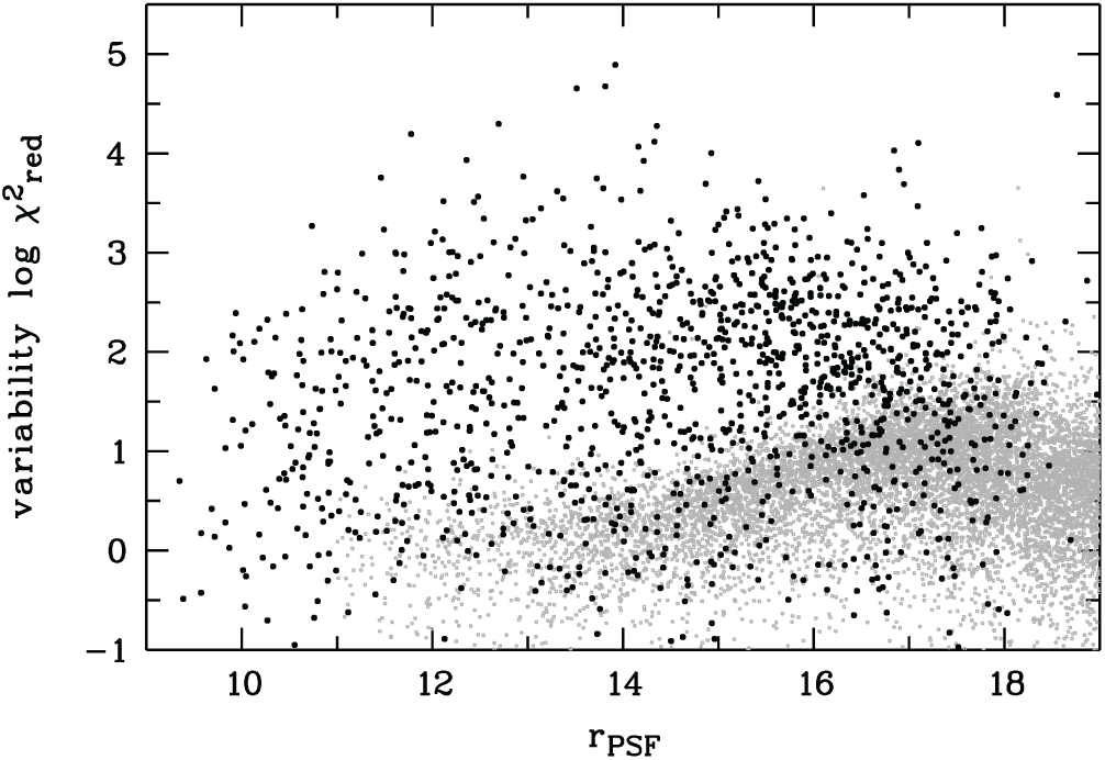
Figure 15. Significance of variability detected among DR2 repeat measurements: we compare a random sample (grey) taken from a small sky area with 1% of the variable source catalogue VSX (large black dots); the plotted variability index is the reduced $\chi^2$
for the set of DR2 photometry being consistent with a constant source, assuming formal flux errors.
$\chi^2$
for the set of DR2 photometry being consistent with a constant source, assuming formal flux errors.
The six-filter SED of variable objects in the master table can be entirely wrong, because filters are observed at different times and clipped for outliers from a median estimate in the distil process. In Figure 16, we compare a known variable star of type RR Lyrae to a random star seen as not varying. The SED of the variable star is plotted from the photometry table for two epochs with Shallow Survey photometry that captures all six filters within a few minutes, while the non-varying star is represented with three to four (depending on filter) epochs. Error bars on magnitudes are mostly too small to be visible, and horizontal error bars represent the filter FWHM.
Table 2. Example of a moving object: multiple appearances of the dwarf planet Pluto in the master table.
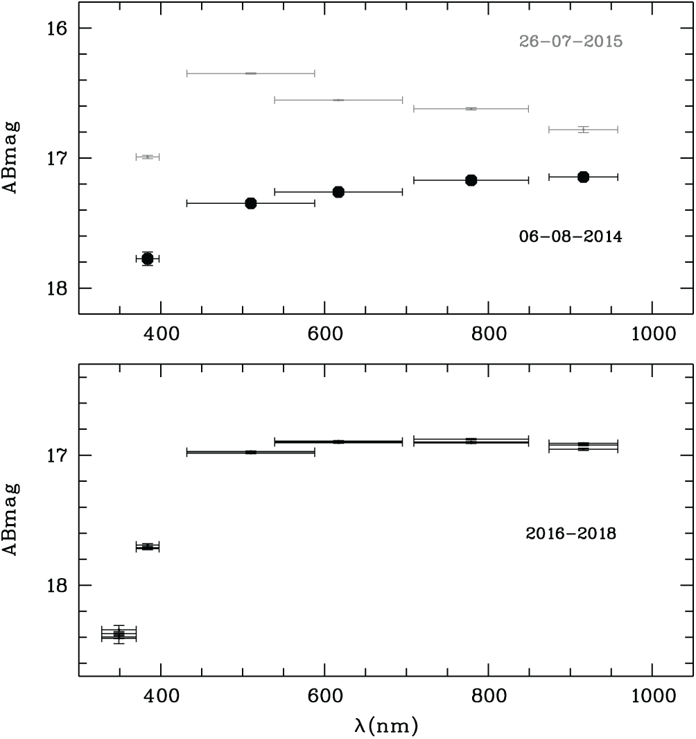
Figure 16. Example SEDs of two stars. Top: a known RR Lyrae star (OBJECT_ID 533362) easily recognisable as variable already in the Shallow Survey photometry (two epochs shown). Bottom: a star (OBJECT_ID 97057927) seen as not varying even with the better precision of the Main Survey (3 to 4 epochs per filter shown).
3.7. Moving and transient objects
Some objects in the master table have only one detection, although that region has been visited multiple times. This includes asteroids and dwarf planets that will be seen at different times in different sky locations, as well as transients that are stable in location but have such high variability amplitudes that they exceed the detection threshold of our imaging only on one occasion. The latter category includes flares on M dwarf stars that are too faint in quiescent state, as well as novae and supernovae.
Here, we note two examples: first, the 14th magnitude dwarf planet Pluto appears five times in the master table between July 2014 and April 2017 (see Table 2). A second, noteworthy, case was identified while selecting M dwarf flares from DR1 (Chang et al. in preparation): an apparent super-flare was seen in an M giant (OBJECT_ID 282264432 in DR2) on 2014 June 18, that seemed to brighten the star to $g\approx 10.7$
mag relative to the other detections around 15 mag. This event turned out to be a chance blend of the star with the
$g\approx 10.7$
mag relative to the other detections around 15 mag. This event turned out to be a chance blend of the star with the $V=10.6$
mag Inner Main Belt asteroid (230) Athamantis, which was moving about half an arcsec min–1.Footnote f Figure 17 shows the time/filter sequence of the Shallow Survey visit to the target location on 2014 June 18 around 16:40 UT, where the middle of the first and last exposures are separated by 3 min. Due to the motion, the u and v centroids differ from the star’s own location such that blended uv magnitudes appear in a separate entry in the master table with OBJECT_ID 282264433.
$V=10.6$
mag Inner Main Belt asteroid (230) Athamantis, which was moving about half an arcsec min–1.Footnote f Figure 17 shows the time/filter sequence of the Shallow Survey visit to the target location on 2014 June 18 around 16:40 UT, where the middle of the first and last exposures are separated by 3 min. Due to the motion, the u and v centroids differ from the star’s own location such that blended uv magnitudes appear in a separate entry in the master table with OBJECT_ID 282264433.
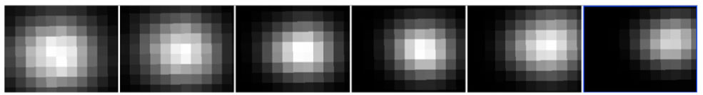
Figure 17. Time/filter sequence of the Shallow Survey visit from 18 June 2014 to the $g\approx 15$
M star with object ID 282264432. Pixel scale is the usual
$g\approx 15$
M star with object ID 282264432. Pixel scale is the usual $\sim 0.5$
arcsec. In these images, the dominant source here is actually the
$\sim 0.5$
arcsec. In these images, the dominant source here is actually the $V=10.6$
mag asteroid (230) Athamantis, which was moving with
$V=10.6$
mag asteroid (230) Athamantis, which was moving with $\sim 0.5$
arcsec per minute. From left to right the filters run along the usual Shallow Survey sequence uvgriz, and the middle of the first and last exposure are separated by 177 s.
$\sim 0.5$
arcsec per minute. From left to right the filters run along the usual Shallow Survey sequence uvgriz, and the middle of the first and last exposure are separated by 177 s.
3.8. Images and CCDs tables
The image table lists dates, positions, exposure times, and quality indicators of each individual telescope exposure. It can be used to differentiate between Shallow Survey and Main Survey images, based on the column IMAGE_TYPE, which is ‘fs’ for the Shallow SurveyFootnote g and ‘ms’ for the Main Survey, or based on EXP_TIME, which is 100 s for the Main Survey but shorter for the Shallow Survey. Images are identified by a unique IMAGE_ID, which encodes roughly the UT date and time of the shutter opening for the exposure in the format YYYYMMDDhhmmss. While the value is rounded to 1 s, it is not actually the time stamp for the exposure start: it is on average 2 s earlier than the exposure start and extreme values in DR2 range from $-11$
to
$-11$
to $+9$
s. (The DATE column contains the actual MJD at the start of the exposure.) Image IDs are listed for every object detection in the photometry table.
$+9$
s. (The DATE column contains the actual MJD at the start of the exposure.) Image IDs are listed for every object detection in the photometry table.
The ccds table contains every valid CCD of every exposure, and thus nearly 32 times as many rows as the images table. Occasionally, CCDs will be missing for some exposures, either because an adequate World Coordinate System (WCS) solution could not be determined or because the read-out amplifiers failed. The COVERAGE column defines the polygon of a CCD’s footprint, and could be used to check whether a known target location has fallen on a CCD that is part of the data release. This information can be used to investigate non-detections of known targets. An alternative approach for a small number of targets is to visually inspect small images served by the cut-out service, which will return all release images at the target location.
4. DR2 data access
Access to DR2 catalogues and images is provided through the SkyMapper node of the All-Sky Virtual Observatory (ASVO), a framework that builds upon the standards of the International Virtual Observatory Alliance (IVOA). Direct access to the tables and image cut-outs is possible using the Table Access and Simple Image Access Protocols (TAP and SIAP), and a Simple Cone Search (SCS) functionality enables position-based object searches. The SkyMapper websiteFootnote h augments those services with an ‘object viewer’ summarising the key information for each object in the master table, a ‘spectrum viewer’ to display associated spectroscopic data (initially with the 6dFGS spectra, and expanding to include other data sets), and a User Forum for obtaining help and posting tips for others.
The changes from the DR1 catalogue structure described by Wolf et al. (Reference Wolf, Onken and Luvaul2018a) include the following:
1. The master table adds a measure of the local source density (the number of master table sources within 15 arcsec), a per-filter count of the number of observations sigma-clipped from the final estimate of the PSF magnitude, a per-filter reduced
$\chi^2$
statistic for the source being non-variable, and a flag indicating for each of the six filters whether the PSF magnitudes are likely affected by close neighbours at more than a 1% level.2. The master table drops the shape measurements provided in DR1, as their robust estimates are difficult with the mix of exposure times and seeing conditions, and drops the visit counts in each filter, since the different photometric depths of the Main Survey and Shallow Survey render such measures difficult to construct in a meaningful manner.
3. The cross-matching to external catalogues now includes SkyMapper DR1, 2MASS, AllWISE, ATLAS Refcat2, GALEX GUVcat, Gaia DR2, PS1 DR1, and UCAC4. The column containing the second-closest 2MASS source has been dropped from the master table in favour of the second-closest Gaia DR2 source. The 2MASS cross-matching has also been restricted to the PSC, allowing the column specifying the catalogue to be omitted. Instead, it is Gaia DR2 for which we record the two closest matches, as Gaia’s superb resolution can flag sources blended in SkyMapper.
4. A number of smaller external catalogues have been updated to include their closest DR2 cross-matches: 2dFGRS, 2dFLenS, 2MRS, 2QZ/6QZ, 6dFGS, GALAH, HES QSO, Milliquas, and VSX.
5. Since DR2 includes both Main Survey and Shallow Survey images, the name of the photometric table has been generalised to photometry.
6. The photometry table adds two columns: a boolean indicator of whether a particular measurement contributed to the clipped mean magnitude in the master table, and a
$\chi^2$
value for that observation relative to the clipped mean magnitude.


5. Future data releases
The next data release will contain more images and better sky coverage for the Main Survey, as well as co-added sky tiles, where we homogenise the PSFs of images and then re-register and co-add them within filters. The co-added tiles will combine data from both the Main Survey and the Shallow Survey to capture the depth of the images while using shallow data on pixels where deep images are saturated, providing images with wide dynamic range and consistent PSFs across the filters.
In the future, we will also do source-finding on co-added frames, which will give us deeper detections than now; presently, our completeness is limited by detections in individual images even though the distilled photometry has relatively low errors due to the combination of all good detections into distilled magnitudes. Forced-position photometry then becomes possible as well.
Irrespective of co-added frames, we aim to include PSF magnitudes that are based on two-dimensional PSF-fitting instead of 1D growth curves, and are thus more reliable in crowded fields or generally for objects with close neighbours.e plan processing enhancements such as astrometry tied to Gaia DR2 as a reference frame and better fitting of electronic interference and CCD bias, especially in areas covered by large galaxies and extended nebulae, where at present the bias is incorrect, causing excess noise and oversubtraction of the background. This is relevant for the creation of high-quality co-added images of galaxies and accurate SEDs of large galaxies.
Finally, we plan to update the photometric calibration: presently, the calibration uses a transformation from Gaia to SkyMapper that assumes a single-parameter family of stars. Especially in the u and v filters, however, colours depend explicitly on metallicity and stellar population gradients across the sky can cause artificial zero-point drifts. These may be removed by an iterative approach that fits the metallicity from the photometry (e.g. Casagrande et al. Reference Casagrande, Wolf and Mackey2019; Huang et al. Reference Huang2019) and thus refines the zero-point table.
At smaller spatial scale, we will tidy up the calibration by improving our flat fields, which currently have issues at the perimeter of the mosaic and can be wrong by up to 5% in the very corners. However, overall the internal reproducibility of flux measurements of bright stars shows already an RMS scatter of only 1% in the uv filters and 0.7% in griz.
The main advantages of using DR2 over DR1 are the improved zero-point calibration and the availability of deeper Main Survey images on part of the hemisphere, both of which enhance the utility of the SMSS for extragalactic research and for Galactic archaelogy studies. We note in particular that the i and z filters cover $\sim 90$
% of the hemisphere already, although not yet at the final number of visits and depth.
$\sim 90$
% of the hemisphere already, although not yet at the final number of visits and depth.
Acknowledgements
The national facility capability for SkyMapper has been funded through ARC LIEF grant LE130100104 from the Australian Research Council, awarded to the University of Sydney, the Australian National University, Swinburne University of Technology, the University of Queensland, the University of Western Australia, the University of Melbourne, Curtin University of Technology, Monash University, and the Australian Astronomical Observatory. Parts of this project were conducted by the Australian Research Council Centre of Excellence for All-sky Astrophysics (CAASTRO), through project number CE110001020. BPS acknowledges support from the ARC Laureate Fellowship FL0992131. LS expresses thanks for support by the China Postdoctoral Science Foundation (2018M641067). We acknowledge support from the ARC Discovery Projects program, most recently through DP150103294 (GDC, MSB, DM). DM also acknowledges support from an ARC Future Fellowship FT160100206. Development and support for the SkyMapper node of the ASVO has been funded in part by Astronomy Australia Limited (AAL) and the Australian Government through the Commonwealth’s Education Investment Fund (EIF) and National Collaborative Research Infrastructure Strategy (NCRIS), particularly the National eResearch Collaboration Tools and Resources (NeCTAR) and the Australian National Data Service Projects (ANDS). The National Computational Infrastructure (NCI), which is supported by the Australian Government, has contributed resources and services to this project and hosts the SkyMapper node of the ASVO. We acknowledge the Gamilaroi people as the traditional owners of the land on which the SkyMapper Telescope stands.
We thank the referee for comments that improved the quality of the manuscript. We thank John Tonry and Luca Casagrande for extensive discussions that led to the improved photometric zero-point calibration of DR2. We thank Marc White, Jon Smillie, Sean Pringle, and Chris Allen for their support of the SkyMapper node of the ASVO. This work has made use of data from the European Space Agency (ESA) mission Gaia Footnote i, processed by the Gaia Data Processing and Analysis ConsortiumFootnote j (DPAC). Funding for the DPAC has been provided by national institutions, in particular the institutions participating in the Gaia Multilateral Agreement. This publication makes use of data products from the Two Micron All Sky Survey, which is a joint project of the University of Massachusetts and the Infrared Processing and Analysis Center/California Institute of Technology, funded by the National Aeronautics and Space Administration and the National Science Foundation. The Pan-STARRS1 Surveys (PS1) and the PS1 public science archive have been made possible through contributions by the Institute for Astronomy, the University of Hawaii, the Pan-STARRS Project Office, the Max-Planck Society and its participating institutes, the Max Planck Institute for Astronomy, Heidelberg and the Max Planck Institute for Extraterrestrial Physics, Garching, The Johns Hopkins University, Durham University, the University of Edinburgh, the Queen’s University Belfast, the Harvard-Smithsonian Center for Astrophysics, the Las Cumbres Observatory Global Telescope Network Incorporated, the National Central University of Taiwan, the Space Telescope Science Institute, the National Aeronautics and Space Administration under Grant No. NNX08AR22G issued through the Planetary Science Division of the NASA Science Mission Directorate, the National Science Foundation Grant No. AST-1238877, the University of Maryland, Eotvos Lorand University (ELTE), the Los Alamos National Laboratory, and the Gordon and Betty Moore Foundation. This research made use of Astropy, a community-developed core Python package for Astronomy (Astropy Collaboration, 2013).


