1. Introduction
The Murchison Widefield Array (MWA) is a low-frequency (80–300 MHz) radio interferometer located at the Murchison Radio-astronomy Observatory (MRO) in Western Australia, the site of the future low-band Square Kilometre Array (SKA-Low). The array was built with four primary science goals (for a full review, see Bowman et al. Reference Bowman2013): detection of the Epoch of Reionisation (EoR); galactic and extragalactic (GEG) science; time domain astrophysics; and solar, heliospheric, and ionospheric (SHI) science. These science drivers motivated a flexible design with 128 electronically beamformed, large field of view (FoV; $25^\circ$
at 150 MHz) antenna tiles, a densely packed core, and smooth uv coverage to nearly 3 km (Tingay et al. Reference Tingay2013a). The MWA has been operational since 2013, and data from the telescope have been used to make progress along each of its science themes.
$25^\circ$
at 150 MHz) antenna tiles, a densely packed core, and smooth uv coverage to nearly 3 km (Tingay et al. Reference Tingay2013a). The MWA has been operational since 2013, and data from the telescope have been used to make progress along each of its science themes.
The EoR collaboration has studied foregrounds and systematics extensively (e.g. Line et al. Reference Line, Webster, Pindor, Mitchell and Trott2017; Carroll et al. Reference Carroll2016; Procopio et al. Reference Procopio2017; Thyagarajan et al. Reference Thyagarajan2015a; Offringa et al. Reference Offringa2016; Jordan et al. Reference Jordan2017; Trott et al. Reference Trott2019), and placed competitive limits on the redshifted 21 cm power spectrum (Beardsley et al. Reference Beardsley2016; Trott et al. Reference Trott2016; Ewall-Wice et al. Reference Ewall-Wice2016; Dillon et al. Reference Dillon2015).
The GEG group has produced the GaLactic and Extragalactic All-sky MWA (GLEAM) catalog of over 300 000 radio sources with declination south of $+30^{\circ}$
(Wayth et al. Reference Wayth2015; Hurley-Walker et al. Reference Hurley-Walker2017), successfully mapped 306 HII regions in the Galaxy (Hindson et al. Reference Hindson2016), detected molecules below 700 MHz (e.g. Tremblay et al. Reference Tremblay, Hurley-Walker, Cunningham, Jones, Hancock, Wayth and Jordan2017), placed limits on the surface brightness of the synchrotron cosmic web (Vernstrom et al. Reference Vernstrom, Gaensler, Brown, Lenc and Norris2017), and mapped the polarised diffuse sky at long wavelengths (Lenc et al. Reference Lenc2016).
$+30^{\circ}$
(Wayth et al. Reference Wayth2015; Hurley-Walker et al. Reference Hurley-Walker2017), successfully mapped 306 HII regions in the Galaxy (Hindson et al. Reference Hindson2016), detected molecules below 700 MHz (e.g. Tremblay et al. Reference Tremblay, Hurley-Walker, Cunningham, Jones, Hancock, Wayth and Jordan2017), placed limits on the surface brightness of the synchrotron cosmic web (Vernstrom et al. Reference Vernstrom, Gaensler, Brown, Lenc and Norris2017), and mapped the polarised diffuse sky at long wavelengths (Lenc et al. Reference Lenc2016).
The MWA has been used to follow up gravitational wave (GW) events (Abbott et al. Reference Abbott2016a) and gamma-ray bursts (Kaplan et al. Reference Kaplan2015 c), place limits on low-frequency fast radio bursts (FRBs; Tingay et al. Reference Tingay2015; Rowlinson et al. Reference Rowlinson2016; Keane et al. Reference Keane2016; Sokolowski et al. Reference Sokolowski2018), detect polarised flares from UV Ceti (Lynch et al. Reference Lynch, Lenc, Kaplan, Murphy and Anderson2017b), survey the southern sky for low-frequency variability (Bell et al. Reference Bell2019), and perform detailed pulsar studies (e.g. Bhat et al. Reference Bhat2014; Bhat et al. Reference Bhat, Ord, Tremblay, McSweeney and Tingay2016; McSweeney et al. Reference McSweeney, Bhat, Tremblay, Deshpande and Ord2017; Meyers et al. Reference Meyers2017; Xue et al. Reference Xue2017; Bell et al. Reference Bell2016; Murphy et al. Reference Murphy2017).
Solar observations require extremely high dynamic range, which has led to new imaging and calibration techniques (Oberoi et al. Reference Oberoi, Sharma and Rogers2017; Mohan & Oberoi Reference Mohan and Oberoi2017). The SHI group has characterised weak nonthermal solar emission (Suresh et al. Reference Suresh2017; Sharma et al. Reference Sharma, Oberoi and Arjunwadkar2018) and detected IPS due to solar wind both serendipitously (Kaplan et al. Reference Kaplan2015a) and with directed observations (Morgan et al. Reference Morgan2018). One of the most exciting discoveries from the MWA has been the first direct detection of plasma ducts aligned with the Earth’s magnetic field in the ionosphere (Loi et al. Reference Loi2015a).
In addition to being a scientifically flexible instrument, the relatively simple front-end infrastructure and compute-based back-end of the MWA make it a strong candidate for continued investment with upgrades that greatly enhance the capabilities at low cost. Since the initial deployment, the MWA has undergone several upgrades, including the addition of 128 tiles resulting in two distinct configurations (compact and extended) (Wayth et al. Reference Wayth2018), an improved triggering system (Hancock et al. Reference Hancock2019), and a new digital back-end to support the search for extraterrestrial intelligence (SETI). These upgrades have grown the scientific capabilities of the MWA and, in some cases, enable entirely new directions to explore.
The MWA collaboration currently includes 21 partner institutions from 6 countries (Australia, Canada, China, Japan, New Zealand, and the United States). The MWA operates under an Open Skies policy, and any researcher may propose for observing timeFootnote a. In addition, all raw visibility data become open access after an initial proprietary period and can be accessed by the All-Sky Virtual ObservatoryFootnote b.
In this paper, we give a brief overview of changes that have been made to the MWA since its initial deployment (Section 2), and highlight many science opportunities that are enabled by these upgrades, categorised by the four primary science themes that drove the instrument design (Sections 3, 4, 5, and 6). The flexibility of observatory and its general-purpose nature have been key to its success. We recognise not all results will fall neatly within the four science themes, and present some examples of such opportunities in Section 7.
2. Upgrades and improvements
We will refer to the MWA as described in Tingay et al. (2013) and operating 2013–2016 as ‘Phase I’. Beginning mid-2016, 128 tiles were added to the array. We will refer to the array at this stage, along with other upgrades described below as ‘Phase II’.
2.1. Additional tiles
The antenna layout of the MWA was substantially changed with the addition of 128 tiles, for a total of 256 tiles. This upgrade is described fully in Wayth et al. (Reference Wayth2018), and we provide a brief summary here. The 256-input correlator can process 128 dual-polarisation signals at a time, so the array is periodically reconfigured between compact and extended configurations.
2.1.1. Compact configuration
The compact configuration of Phase II consists of 56 tiles from the original Phase I core (including a few tiles an intermediate distance from the centre) and adds two hexagonal (‘hex’) cores of 36 tiles each. The size of the hex cores was chosen to be comparable to the original core, and the spacing was chosen to yield relatively smooth uv coverage to $\sim\!~100\, \text{m}$
. The spacing is also approximately that of the hydrogen epoch of reionisation array (HERA; DeBoer et al. Reference DeBoer2017), which will allow cross checks for EoR science. The layout is shown in Figure 1.
$\sim\!~100\, \text{m}$
. The spacing is also approximately that of the hydrogen epoch of reionisation array (HERA; DeBoer et al. Reference DeBoer2017), which will allow cross checks for EoR science. The layout is shown in Figure 1.
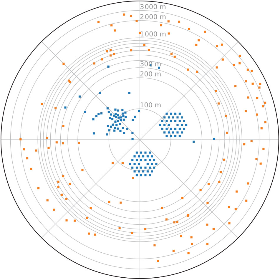
Figure 1. The compact and extended configurations of the Phase II MWA. The blue and orange squares show the tiles which are correlated in the compact and extended configurations, respectively. Note the linear radial scale within 200 m to show the dense pseudo-random/redundant hybrid core, and logarithmic radial scale beyond to capture the nearly 6 km diameter.
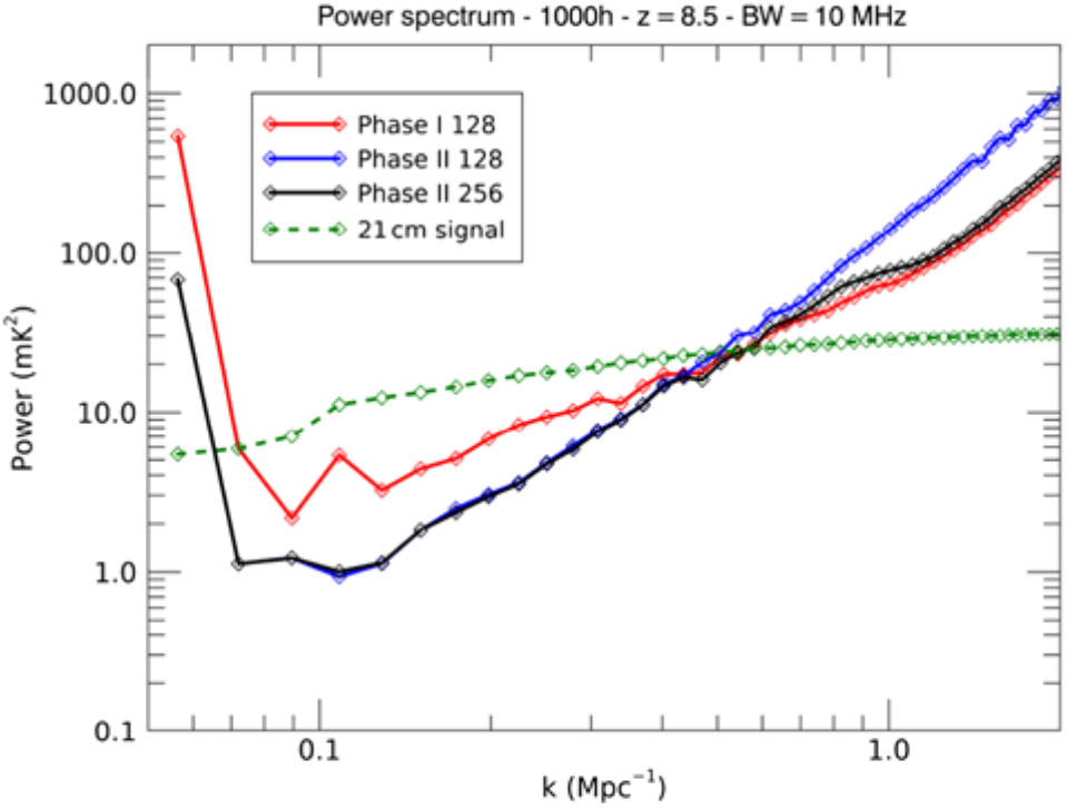
The primary motivation for the compact configuration is to increase surface brightness sensitivity relative to the Phase I array. The net effect is a significant increase in sensitivity to diffuse signals like the 21 cm signal from the EoR. Figure 2 demonstrates the thermal noise levels achievable in a power spectrum measurement of the 21 cm signal for Phase I (red), Phase II (blue), and a hypothetical Phase II array with all 256 tiles correlated (black). Phase II achieves lower noise levels by a factor of $\sim\! 2$
–5 (in
$\sim\! 2$
–5 (in $\text{mK}^2$
) compared with Phase I over a wide range of scales. Comparisons with other facilities such as HERA, the Low-Frequency Array (LOFAR), and the Precision Array for Probing the Epoch of Reionisation (PAPER) can be found in DeBoer et al. (Reference DeBoer2017) (their Figure 4) and the appendix of Pober et al. (Reference Pober2014).
$\text{mK}^2$
) compared with Phase I over a wide range of scales. Comparisons with other facilities such as HERA, the Low-Frequency Array (LOFAR), and the Precision Array for Probing the Epoch of Reionisation (PAPER) can be found in DeBoer et al. (Reference DeBoer2017) (their Figure 4) and the appendix of Pober et al. (Reference Pober2014).

Figure 2. Typical EoR power spectrum model at 150 MHz with associated noise levels available to the Phase I and Phase II arrays with 1000 h observation. ‘Phase II 256’ represents the result from a future MWA upgrade where all 256 tiles are used simultaneously. (From Wayth et al. Reference Wayth2018).
Beyond the increased surface brightness sensitivity, the substantial number of redundant baselines serves a dual-purpose. First, they enable coherent addition of redundant visibilities without requiring gridding or imaging. This redundancy can ultimately serve to increase the sensitivity of a class of non-imaging EoR power spectrum estimators like the delay spectrum approach pioneered by PAPER (Parsons et al. Reference Parsons, Pober, McQuinn, Jacobs and Aguirre2012a,b). For a pedagogical description of imaging and non-imaging EoR power spectrum estimators, see Morales et al. (Reference Morales, Beardsley, Pober, Barry, Hazelton, Jacobs and Sullivan2019). Second, redundancy enables a new class of interferometric calibration techniques that derive antenna-based gains by minimising deviations between visibilities from redundant baselines (Wieringa Reference Wieringa1992; Liu et al. Reference Liu, Tegmark, Morrison, Lutomirski and Zaldarriaga2010; Zheng et al. Reference Zheng2014). The Phase II compact configuration is somewhat unique, however, in retaining a large number of non-redundant baselines to preserve a high-fidelity point spread function (PSF) for imaging and image-based calibration.
2.1.2. Extended configuration
The extended configuration of Phase II consists of 72 tiles from the original Phase I array and 56 new long baseline tiles (Figure 1). The extended layout nearly doubles the longest baselines (from 3 to 5.3 km), resulting in a resolution of $\sim\!1.3\,\text{arcmin}$
at 154 MHz. Franzen et al. (Reference Franzen2016) estimated the Phase I classical confusion limit to be
$\sim\!1.3\,\text{arcmin}$
at 154 MHz. Franzen et al. (Reference Franzen2016) estimated the Phase I classical confusion limit to be $\sim1.7~\text{mJy}$
at 154 MHz, and the improved resolution is expected to reduce this by a factor of 5–10.
$\sim1.7~\text{mJy}$
at 154 MHz, and the improved resolution is expected to reduce this by a factor of 5–10.
In addition, the naturally weighted PSF of the extended configuration is significantly smoother than that of the Phase I array, owing to the lack of a dense core and instead a more uniform sampling of the uv plane (Wayth et al. Reference Wayth2018). Therefore, we expect lower sidelobe confusion noise, and improved point source sensitivity.
2.2. Digital back-ends
2.2.1. Correlator data rate
The data rate of the archive restricted the correlator during Phase I to a time–frequency resolution set by
 $$\tau \Delta f \mathbin{\lower.3ex\hbox{$\buildrel>\over
{\smash{\scriptstyle\sim}\vphantom{_x}}$}} 2{\mkern 1mu} 000$$
, where
$$\tau \Delta f \mathbin{\lower.3ex\hbox{$\buildrel>\over
{\smash{\scriptstyle\sim}\vphantom{_x}}$}} 2{\mkern 1mu} 000$$
, where $\tau$
is the visibility integration time and
$\tau$
is the visibility integration time and $\Delta f$
is the bandwidth of a single frequency channel. However, the longer baselines of the extended configuration of Phase II necessitated finer time–frequency resolution. This was made possible by implementing a lossless in-situ compression on the visibilities (Kitaeff Reference Kitaeff, Taylor and Rosolowsky2015) and an expansion of the onsite archive system. The result is a factor of 4 increase in possible output data rate, for example, typical observations in the extended configuration have frequency and time resolution of 10 kHz and 0.5 s, respectively.
$\Delta f$
is the bandwidth of a single frequency channel. However, the longer baselines of the extended configuration of Phase II necessitated finer time–frequency resolution. This was made possible by implementing a lossless in-situ compression on the visibilities (Kitaeff Reference Kitaeff, Taylor and Rosolowsky2015) and an expansion of the onsite archive system. The result is a factor of 4 increase in possible output data rate, for example, typical observations in the extended configuration have frequency and time resolution of 10 kHz and 0.5 s, respectively.
2.2.2. Voltage capture buffer
The MWA voltage capture system (VCS; Tremblay et al. Reference Tremblay2015) facilitates recording of raw antenna voltage data (before correlation and tied-array beamforming) at
 $${\rm{100\mu s}}$$
and 10 kHz resolution. This capability has been exploited for a variety of pulsar science applications such as investigating pulsar emission physics and studies of millisecond pulsars (e.g. Bhat et al. Reference Bhat, Ord, Tremblay, McSweeney and Tingay2016; McSweeney et al. Reference McSweeney, Bhat, Tremblay, Deshpande and Ord2017; Meyers et al. Reference Meyers2017; Bhat et al. Reference Bhat2018; Meyers et al. Reference Meyers2018). A new feature has enabled buffering voltage data up to 150 s, which can be recorded after receiving a trigger (Subsection 2.3). In this mode, instead of recording directly to disk, the voltages are stored in a ring buffer in the on-board memory of the VCS servers (Hancock et al. Reference Hancock2019). The voltages are kept in the rolling memory buffer for as long as possible (depending on the available memory) on a first-in-first-out basis.
$${\rm{100\mu s}}$$
and 10 kHz resolution. This capability has been exploited for a variety of pulsar science applications such as investigating pulsar emission physics and studies of millisecond pulsars (e.g. Bhat et al. Reference Bhat, Ord, Tremblay, McSweeney and Tingay2016; McSweeney et al. Reference McSweeney, Bhat, Tremblay, Deshpande and Ord2017; Meyers et al. Reference Meyers2017; Bhat et al. Reference Bhat2018; Meyers et al. Reference Meyers2018). A new feature has enabled buffering voltage data up to 150 s, which can be recorded after receiving a trigger (Subsection 2.3). In this mode, instead of recording directly to disk, the voltages are stored in a ring buffer in the on-board memory of the VCS servers (Hancock et al. Reference Hancock2019). The voltages are kept in the rolling memory buffer for as long as possible (depending on the available memory) on a first-in-first-out basis.
2.2.3. Breakthrough listen
Although replacement of the correlator hardware was not included in the Phase II upgrades, work is currently underway to enable much higher frequency resolution and more flexible beamforming. Additionally, a fibre link from the MRO to Curtin University means that raw voltage data can be accessed offsite, enabling easier deployment of commensal instruments that can produce beams and spectra within the primary FOV, independent of the science user who is controlling the primary beam pointing. The breakthrough listen (BL; Worden et al. Reference Worden2017) team has deployed hardware to Curtin as part of a pilot program to perform experiments to SETI (Section 7.2). The BL hardware will also serve as a general purpose instrument for targets such as fast transients and pulsars—in essence an enhanced version of the existing VCS.
2.3. Rapid-response triggering
Recently, an upgraded automatic observation triggering system has been deployed on the MWA. Hancock et al. (Reference Hancock2019) describe the triggering system in detail, while we provide a brief overview here. The system handles alerts from the Virtual Observatory Event standard (VOEvent; Seaman et al. Reference Seaman2011) and can interrupt ongoing observations based on project priorities set ahead of time by the MWA director. Observations can be triggered in one of three modes: (1) using the regular visibility correlator; (2) using the VCS to capture voltage data; or (3) if the telescope is already in a buffered capture mode, the trigger can cause the buffer to be drained to disk. Due to scheduling constraints and processing time, the first two modes have a latency of 6–14 s from the time the alert is received, while the third mode can have an effective negative latency because it can hold up to 150 s of buffered data.
The remaining sections of this article will recap some of the progress to date in the MWA’s key science themes and discuss further science opportunities enabled by the Phase II upgrades.
3. Epoch of reionisation
The MWA EoR project collected more than 2 000 h of data during the 4 yr of Phase I. These data were observed in pointed and zenith drift mode, and concentrated primarily on three southern fields away from the Galactic plane. Jacobs et al. (Reference Jacobs2016) describe the observational parameters and data analysis pipelines. Subsets of these data were published to place upper limits on the EoR spatial brightness temperature fluctuation power spectrum at $z=7.0-8.6$
(Barry et al. Reference Barry2019; Trott et al. Reference Trott2016; Beardsley et al. Reference Beardsley2016; Paul et al. Reference Paul2016; Ewall-Wice et al. Reference Ewall-Wice2016; Dillon et al. Reference Dillon2015), as shown graphically in Figure 3 together with expected signal strengths from 21cmFAST (Mesinger et al. Reference Mesinger, Furlanetto and Cen2011). A larger body of research used these data to design, test, and improve data analysis methodology and calibration schemes (Barry et al. Reference Barry, Hazelton, Sullivan, Morales and Pober2016; Line et al. Reference Line, Webster, Pindor, Mitchell and Trott2017; Procopio et al. Reference Procopio2017; Carroll et al. Reference Carroll2016; Offringa et al. Reference Offringa2016), and to explore aspects of the data set and instrument that affect the potential to detect the EoR signal (Jordan et al. Reference Jordan2017; Lenc et al. Reference Lenc2017; Loi et al. Reference Loi2016; Pober et al. Reference Pober2016). The combined output of these analyses has demonstrated that exquisite knowledge of the sky, instrument, and data processing methodology is crucial for successful and robust EoR detection. As such, instrumentation advances such as the hexagonal redundant sub-arrays of Compact Phase II, combined with the long baselines and excellent snapshot uv-coverage of the extended configuration, afford new avenues for data calibration and sky model building.
$z=7.0-8.6$
(Barry et al. Reference Barry2019; Trott et al. Reference Trott2016; Beardsley et al. Reference Beardsley2016; Paul et al. Reference Paul2016; Ewall-Wice et al. Reference Ewall-Wice2016; Dillon et al. Reference Dillon2015), as shown graphically in Figure 3 together with expected signal strengths from 21cmFAST (Mesinger et al. Reference Mesinger, Furlanetto and Cen2011). A larger body of research used these data to design, test, and improve data analysis methodology and calibration schemes (Barry et al. Reference Barry, Hazelton, Sullivan, Morales and Pober2016; Line et al. Reference Line, Webster, Pindor, Mitchell and Trott2017; Procopio et al. Reference Procopio2017; Carroll et al. Reference Carroll2016; Offringa et al. Reference Offringa2016), and to explore aspects of the data set and instrument that affect the potential to detect the EoR signal (Jordan et al. Reference Jordan2017; Lenc et al. Reference Lenc2017; Loi et al. Reference Loi2016; Pober et al. Reference Pober2016). The combined output of these analyses has demonstrated that exquisite knowledge of the sky, instrument, and data processing methodology is crucial for successful and robust EoR detection. As such, instrumentation advances such as the hexagonal redundant sub-arrays of Compact Phase II, combined with the long baselines and excellent snapshot uv-coverage of the extended configuration, afford new avenues for data calibration and sky model building.

Figure 3. Upper limits (95% confidence) on the power spectrum of brightness temperature fluctuations from the Epoch of Reionisation at their respective redshifts and k-modes, published using MWA Phase I data (filled triangles): Barry et al. (Reference Barry2019) (purple), Trott et al. (Reference Trott2016) (red), Beardsley et al. (Reference Beardsley2016) (green), Dillon et al. (Reference Dillon2015) (black), Dillon et al. (Reference Dillon2014) (blue), and Ewall-Wice et al. (Reference Ewall-Wice2016) (orange). Leading results from other telescopes are shown with unfilled squares: Paciga et al. (Reference Paciga2013) (GMRT, orange), Patil et al. (Reference Patil2017) (LOFAR, purple), and Kolopanis et al. (Reference Kolopanis2019) (PAPER, red). Expected signal strength using 21cmFAST for the same redshifts and scales is shown with corresponding circles (Mesinger et al. Reference Mesinger, Furlanetto and Cen2011).
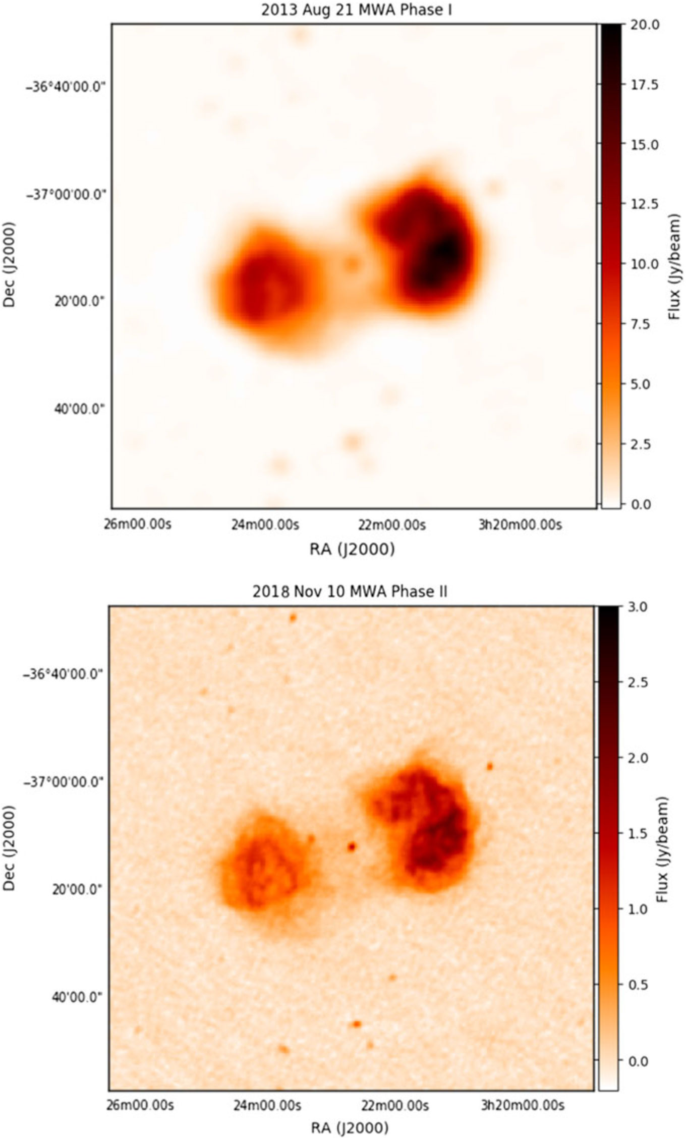
Figure 4. Comparison of MWA Phase I and Phase II extended array images of Fornax A. The extended array resolves the finer structures in the lobes of this source while over-resolving the bright, more diffuse emission. The MWA Phase I image adapted from McKinley et al. (Reference McKinley2015).
3.1. Redundant calibration
Precision calibration is one of the most significant challenges facing EoR experiments, as spurious spectral structure in calibration solutions can spread foreground power through k space (see, e.g., Yatawatta Reference Yatawatta2015; Thyagarajan et al. Reference Thyagarajan2015b; Thyagarajan et al. Reference Thyagarajan2015 c; Barry et al. Reference Barry, Hazelton, Sullivan, Morales and Pober2016; Dillon et al. Reference Dillon2018). Barry et al. (Reference Barry, Hazelton, Sullivan, Morales and Pober2016), in particular, demonstrate how calibration algorithms that rely on a sky model can introduce contamination into the EoR window when the sky model is incomplete. Redundant calibration (Wieringa Reference Wieringa1992; Liu et al. Reference Liu, Tegmark, Morrison, Lutomirski and Zaldarriaga2010; Zheng et al. Reference Zheng2014) therefore presents an appealing alternative for EoR experiments, because it only requires a sky model to constrain a subset of the calibration parameters. Because of its unique layout, with substantial numbers of both redundant and non-redundant baselines, the compact configuration of Phase II is a valuable testing ground for comparing redundant and sky-based calibration techniques in the pursuit of EoR science. Li et al. (Reference Li2018) conducted just such a study, developing redundant calibration techniques for the Phase II compact array and comparing them with the sky-based calibration techniques similar to those used in Beardsley et al. (Reference Beardsley2016). They find that applying redundant and sky-based calibration techniques in tandem yields small but significant reductions in foreground contamination of the EoR power spectrum.
A number of other theoretical studies are under way to determine optimal strategies for calibrating data from the compact array for EoR science, augmenting existing literature of results from other arrays (Thyagarajan et al. Reference Thyagarajan, Carilli and Nikolic2018; Orosz et al. Reference Orosz, Dillon, Ewall-Wice, Parsons and Thyagarajan2018). Joseph et al. (Reference Joseph, Trott and Wayth2018) demonstrate how the flux density distribution of the sky can affect redundant calibration techniques, despite the lack of explicit reference to a sky model. Byrne et al. (Reference Byrne2019) study the subset of parameters that cannot be constrained by redundant calibration and show how sky model incompleteness errors still affect these terms, which, in turn, introduce contamination into the EoR window. Continued studies of redundant and sky-based calibration techniques using the compact array may be invaluable for the future of 21 cm science, as a combination of both techniques may be necessary to mitigate the limitations of each one independently.
3.2. 21 cm power spectra
As stated in Section 2, the compact configuration of Phase II provides a significant increase in surface brightness sensitivity over the Phase I configuration. Figure 2 shows how this upgrade translates into expected improvements in the sensitivity of the array to the power spectrum of the EoR. Li et al. (Reference Li2018) present the first preliminary power spectra from Phase II, using a few hours of data, and show that existing power spectrum pipelines from Phase I like FHD/ $\epsilon$
ppsilon (Jacobs et al. Reference Jacobs2016) can be adapted and applied to Phase II data. Work is now in progress to process the first season of Phase II data and produce a deep power spectrum limit comparable to Beardsley et al. (Reference Beardsley2016). Other efforts are under way to analyse data taken from Phase II in a drift scan mode using alternate power spectrum pipelines.
$\epsilon$
ppsilon (Jacobs et al. Reference Jacobs2016) can be adapted and applied to Phase II data. Work is now in progress to process the first season of Phase II data and produce a deep power spectrum limit comparable to Beardsley et al. (Reference Beardsley2016). Other efforts are under way to analyse data taken from Phase II in a drift scan mode using alternate power spectrum pipelines.
3.3. LoBES and diffuse emission
The MWA EoR fields were chosen based on their low sky temperature and preferable elevation angles for night-time observing. Yet, these fields are imperfect: the large FOV of the MWA, extending beyond $40^{\circ}$
in the sidelobes, makes it difficult to avoid all bright extended radio galaxies and the Galactic plane entirely. Therefore, the MWA EoR fields contain several bright, extended sources (e.g. Hydra A, Fornax A, 3C444) located either at the edges of the MWA primary beam or in the primary beam sidelobes (Jacobs et al. Reference Jacobs2016). These sources are expected to produce significant foreground contamination in the EoR power spectrum, with Procopio et al. (Reference Procopio2017) estimating that mis-modelling the brightest 10 sources contributes
$40^{\circ}$
in the sidelobes, makes it difficult to avoid all bright extended radio galaxies and the Galactic plane entirely. Therefore, the MWA EoR fields contain several bright, extended sources (e.g. Hydra A, Fornax A, 3C444) located either at the edges of the MWA primary beam or in the primary beam sidelobes (Jacobs et al. Reference Jacobs2016). These sources are expected to produce significant foreground contamination in the EoR power spectrum, with Procopio et al. (Reference Procopio2017) estimating that mis-modelling the brightest 10 sources contributes $>$
90% of the power bias. Trott & Wayth (Reference Trott and Wayth2017) compared bias in the EoR power spectrum from poorly resolved extended sources, showing that detection of the EoR with the MWA would require the spatial resolution of the extended MWA combined with some TGSS data from the Giant Metrewave Radio Telescope (GMRT).
$>$
90% of the power bias. Trott & Wayth (Reference Trott and Wayth2017) compared bias in the EoR power spectrum from poorly resolved extended sources, showing that detection of the EoR with the MWA would require the spatial resolution of the extended MWA combined with some TGSS data from the Giant Metrewave Radio Telescope (GMRT).
The frequency dependence of an interferometer’s PSF becomes stronger far from the pointing centre and so sources located far from the primary FOV produce more foreground contamination than sources located in the centre of the primary beam (Thyagarajan et al. Reference Thyagarajan2015a; Trott et al. Reference Trott, Wayth and Tingay2012). Pober et al. (Reference Pober2016) showed that subtracting a foreground model that includes sources in both the main FOV and the first sidelobe is found to reduce the contamination in EoR power spectrum by several per cent relative to a model including only the sources in the main field of view, and other recent work has studied the impact of incomplete sky models on calibration (Patil et al. Reference Patil2016; Barry et al. Reference Barry, Hazelton, Sullivan, Morales and Pober2016). Additionally, detailed models for extended sources and double sources are required for foreground modelling and subtraction, as subtracting these sources as point sources leaves residual excess power that has the potential to introduce bias into the EoR power spectrum (Procopio et al. Reference Procopio2017; Trott & Wayth Reference Trott and Wayth2017).
In an effort to improve the source models of both point and extended sources in the MWA primary beam sidelobes of the EoR0 (Right Ascension (RA) $=$
0.00 h, Declination
$=$
0.00 h, Declination $\text{(Dec)}\,=\,{-27}^{\circ}$
) and EoR1
$\text{(Dec)}\,=\,{-27}^{\circ}$
) and EoR1 $\text{(RA}\,=\,{4.00}\,\text{h, Dec}\,=\,{-27}^{\circ}\text{)}$
fields, members of the MWA EoR team are conducting the Long Baseline Epoch of Reionisation Survey (LoBES). This survey consists of multi-frequency (four bands covering 103–230 MHz) observations of EoR0, EoR1, and their eight neighbouring fields using the MWA Phase II extended array. Observations were undertaken in Semester 2017B and are being calibrated for future publication. Observations of the EoR0 and EoR1 fields using the longer baselines will provide high-resolution uv-components to complement the existing uv-plane sampling of these fields. The neighbouring fields will provide high-resolution observations of troublesome sidelobe sources within the centre of the MWA primary beam, where the primary beam is well modelled (Sutinjo et al. Reference Sutinjo2015). As an example, Figure 4 compares MWA Phase I and Phase II extended array images of Fornax A, highlighting the more complex structure revealed by the higher resolution of the extended array. The longer baselines will also allow for deeper measurements of foreground sources due to the reduced classical confusion limit, expanding the foreground catalogue by a factor of 3–4. Using a model of extragalactic foreground contamination similar to that of Trott et al. (Reference Trott2016), this could reduce the amount of leaked foreground power by an estimated factor of
$\text{(RA}\,=\,{4.00}\,\text{h, Dec}\,=\,{-27}^{\circ}\text{)}$
fields, members of the MWA EoR team are conducting the Long Baseline Epoch of Reionisation Survey (LoBES). This survey consists of multi-frequency (four bands covering 103–230 MHz) observations of EoR0, EoR1, and their eight neighbouring fields using the MWA Phase II extended array. Observations were undertaken in Semester 2017B and are being calibrated for future publication. Observations of the EoR0 and EoR1 fields using the longer baselines will provide high-resolution uv-components to complement the existing uv-plane sampling of these fields. The neighbouring fields will provide high-resolution observations of troublesome sidelobe sources within the centre of the MWA primary beam, where the primary beam is well modelled (Sutinjo et al. Reference Sutinjo2015). As an example, Figure 4 compares MWA Phase I and Phase II extended array images of Fornax A, highlighting the more complex structure revealed by the higher resolution of the extended array. The longer baselines will also allow for deeper measurements of foreground sources due to the reduced classical confusion limit, expanding the foreground catalogue by a factor of 3–4. Using a model of extragalactic foreground contamination similar to that of Trott et al. (Reference Trott2016), this could reduce the amount of leaked foreground power by an estimated factor of $10^{2}-10^{3}$
.
$10^{2}-10^{3}$
.
3.4. 21 cm-LAE cross power spectrum
The cross correlation between the 21 cm signal and the high redshift Lyman- $\alpha$
emitter (LAE) distribution can help to identify the 21 cm signal and enhance the detectability because the foregrounds are expected to have negligible correlation with the LAE distribution (Sobacchi et al. Reference Sobacchi, Mesinger and Greig2016; Lidz et al. Reference Lidz, Zahn, Furlanetto, McQuinn, Hernquist and Zaldarriaga2008). In the absence of foregrounds, the MWA Phase II compact configuration is predicted to have sufficient sensitivity to detect the 21 cm-LAE cross power spectrum (CPS) with an observation of 1 000 h combined with the LAE survey by Subaru Hyper Suprime Cam (HSC) (Kubota et al. Reference Kubota, Yoshiura, Takahashi, Hasegawa, Yajima, Ouchi, Pindor and Webster2018). With realistic models for foregrounds, Yoshiura et al. Reference Yoshiura, Line, Kubota, Hasegawa and Takahashi2018 found that subtraction of 80% of diffuse and 99% of point source foregrounds will be needed to reach a CPS detection at
$\alpha$
emitter (LAE) distribution can help to identify the 21 cm signal and enhance the detectability because the foregrounds are expected to have negligible correlation with the LAE distribution (Sobacchi et al. Reference Sobacchi, Mesinger and Greig2016; Lidz et al. Reference Lidz, Zahn, Furlanetto, McQuinn, Hernquist and Zaldarriaga2008). In the absence of foregrounds, the MWA Phase II compact configuration is predicted to have sufficient sensitivity to detect the 21 cm-LAE cross power spectrum (CPS) with an observation of 1 000 h combined with the LAE survey by Subaru Hyper Suprime Cam (HSC) (Kubota et al. Reference Kubota, Yoshiura, Takahashi, Hasegawa, Yajima, Ouchi, Pindor and Webster2018). With realistic models for foregrounds, Yoshiura et al. Reference Yoshiura, Line, Kubota, Hasegawa and Takahashi2018 found that subtraction of 80% of diffuse and 99% of point source foregrounds will be needed to reach a CPS detection at $k=0.4\,\text{hMpc}^{-1}$
. The removal of these contaminants is an ongoing effort by the MWA collaboration and is aided by innovative Phase II surveys as described in Sections 3.3 and 3.6.
$k=0.4\,\text{hMpc}^{-1}$
. The removal of these contaminants is an ongoing effort by the MWA collaboration and is aided by innovative Phase II surveys as described in Sections 3.3 and 3.6.
The LAE survey is ongoing and, recently, the LAE distribution with partial survey data at z $=$
5.7 and 6.6 has been reported (Ouchi et al. Reference Ouchi2018; Shibuya et al. Reference Shibuya2018a,b; Konno et al. Reference Konno2018). Thus, there is an opportunity for the analysis of 21 cm-LAE cross correlation. Although the areas of sky do not overlap with the MWA EoR fields, the MWA Phase II will observe the HSC fields and can place a competitive limit on the CPS with a relatively short duration of survey because the Compact Phase II has high sensitivity at large scales as shown in Figure 2. Furthermore, the detectability is enhanced when a spectrographic survey by the Prime Focus Spectrograph (PFS) determines the precise redshift of LAEs, and the three-dimensional information is available. The expected sensitivity is shown in Figure 5.
$=$
5.7 and 6.6 has been reported (Ouchi et al. Reference Ouchi2018; Shibuya et al. Reference Shibuya2018a,b; Konno et al. Reference Konno2018). Thus, there is an opportunity for the analysis of 21 cm-LAE cross correlation. Although the areas of sky do not overlap with the MWA EoR fields, the MWA Phase II will observe the HSC fields and can place a competitive limit on the CPS with a relatively short duration of survey because the Compact Phase II has high sensitivity at large scales as shown in Figure 2. Furthermore, the detectability is enhanced when a spectrographic survey by the Prime Focus Spectrograph (PFS) determines the precise redshift of LAEs, and the three-dimensional information is available. The expected sensitivity is shown in Figure 5.
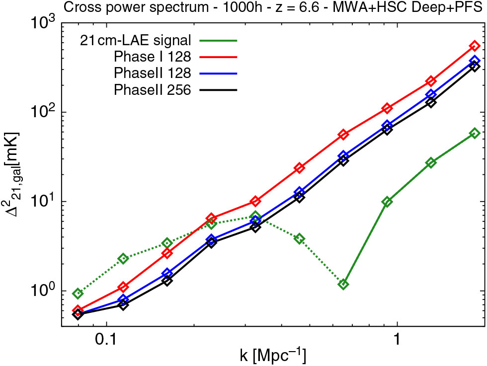
Figure 5. Expected sensitivity to the 21 cm-LAE power spectrum at z $=$
6.6 with an observation of 1 000 h, HSC and PFS survey. The signal is calculated using large-scale radiative transfer simulation of reionisation, which is identical to the simulation used in Kubota et al. (Reference Kubota, Yoshiura, Takahashi, Hasegawa, Yajima, Ouchi, Pindor and Webster2018).
$=$
6.6 with an observation of 1 000 h, HSC and PFS survey. The signal is calculated using large-scale radiative transfer simulation of reionisation, which is identical to the simulation used in Kubota et al. (Reference Kubota, Yoshiura, Takahashi, Hasegawa, Yajima, Ouchi, Pindor and Webster2018).
3.5. 21 cm bispectrum
The bispectrum is the Fourier transform of the three-point correlation function and extracts non-Gaussian information about the 21 cm brightness temperature field that is lost in two-point statistics such as the power spectrum (Watkinson et al. Reference Watkinson, Majumdar, Pritchard and Mondal2017; Watkinson et al. Reference Watkinson, Giri, Ross, Dixon, Iliev, Mellema and Pritchard2019; Mondal et al. Reference Mondal, Bharadwaj, Majumdar, Bera and Acharyya2015; Majumdar et al. Reference Majumdar, Pritchard, Mondal, Watkinson, Bharadwaj and Mellema2018; Yoshiura et al. Reference Yoshiura, Shimabukuro, Takahashi, Momose, Nakanishi and Imai2015). Bispectra are fundamentally formed from closed triplets of interferometric baselines, with equilateral, isosceles, and more generalised triangle configurations encoding information on different scales. The 21 cm bispectrum is difficult to measure with current experiments (Yoshiura et al. Reference Yoshiura, Shimabukuro, Takahashi, Momose, Nakanishi and Imai2015) but allows a fresh approach to treating foregrounds by using the data in a different way to power spectra. In particular, the redundant triangles available in the hexagonal sub-arrays of the Compact Phase II configuration afford a direct bispectrum estimator with increased instantaneous sensitivity. In Trott et al. (Reference Trott2019), a direct bispectrum estimator is applied to 20 h of Phase II data and compared with the estimates using a gridded bispectrum estimator, which uses visibilities gridded to the uv-plane to extract triangles. For stretched isosceles triangles that probe regions of parameter space outside of the wedge foreground contamination region, bispectral estimates are consistent with noise at the 20 h integration stage.
3.6. Large-scale foreground mapping
With a compact core and massively redundant sampling of short baselines, the MWA Phase II is optimised for measurements of the power spectrum on large (many degree) scales. This is in large part because simulations of the 21 cm signal generally suggest that the brightest modes occur on degree scales. Expressed in units of $\text{mK}^{2}\text{Mpc}^{3}$
, the predicted power spectrum, P(k), rises as a power law with decreasing k, while noise remains flat (Mesinger et al. Reference Mesinger, Furlanetto and Cen2011). Unfortunately, a similar spectrum holds for smooth foreground emissions; at degree scales bright galactic power begins to dominate over extragalactic sources (see, e.g., Beardsley et al. Reference Beardsley2016). Accuracy of foreground models used in calibration and foreground subtraction continue to be a limiting factor in 21 cm experiments both interferometric (Barry et al. Reference Barry, Hazelton, Sullivan, Morales and Pober2016) and global (Mozdzen et al. Reference Mozdzen, Mahesh, Monsalve, Rogers and Bowman2019); better maps are needed in the southern hemisphere. However, reconstructing the largest scales probed by an interferometer is difficult where deconvolution must distinguish between primary beam and true structure (Rau & Cornwell Reference Rau and Cornwell2011). Surveys by the Long Wavelength Array (LWA) and the Owens Valley LWA dipole arrays image the largest scales across the visible sky but do not cover the southern hemisphere (Eastwood et al. Reference Eastwood2018; Dowell et al. Reference Dowell, Taylor and Collaboration2015).
$\text{mK}^{2}\text{Mpc}^{3}$
, the predicted power spectrum, P(k), rises as a power law with decreasing k, while noise remains flat (Mesinger et al. Reference Mesinger, Furlanetto and Cen2011). Unfortunately, a similar spectrum holds for smooth foreground emissions; at degree scales bright galactic power begins to dominate over extragalactic sources (see, e.g., Beardsley et al. Reference Beardsley2016). Accuracy of foreground models used in calibration and foreground subtraction continue to be a limiting factor in 21 cm experiments both interferometric (Barry et al. Reference Barry, Hazelton, Sullivan, Morales and Pober2016) and global (Mozdzen et al. Reference Mozdzen, Mahesh, Monsalve, Rogers and Bowman2019); better maps are needed in the southern hemisphere. However, reconstructing the largest scales probed by an interferometer is difficult where deconvolution must distinguish between primary beam and true structure (Rau & Cornwell Reference Rau and Cornwell2011). Surveys by the Long Wavelength Array (LWA) and the Owens Valley LWA dipole arrays image the largest scales across the visible sky but do not cover the southern hemisphere (Eastwood et al. Reference Eastwood2018; Dowell et al. Reference Dowell, Taylor and Collaboration2015).
Reconstruction of large-scale structure with the MWA could be pursued in two ways: mosaicing with many pointings and reconfiguring tile beamforming to widen the FOV. Phase I EoR observations specifically targeted large-scale structure by increasing uv coverage on pointings flanking the primary EoR fields. These observations are currently under study. A similar program with the MWA Phase II, taking advantage of redundancy to supplement calibration models, could potentially offer higher calibration dynamic range as well as a model better matched to Phase II EoR observations. Another method for reconstruction of power on large scales is the m-mode formalism (e.g. Shaw et al. Reference Shaw, Sigurdson, Pen, Stebbins and Sitwell2014; Eastwood et al. Reference Eastwood2018) which is particularly well suited for very large FOV observations where a full 24 sidereal hours are available. This is the goal of the MWA Phase II m-mode project which is currently running a series of observations with all but one dipole per tile disconnected, increasing the FOV to nearly the full sky.
4. Galactic and extragalactic science
The category of GEG science includes a wide variety of targets ranging from molecular transitions in our own Galaxy to large-scale structure in the Universe. The commonality between these objectives lies in the imaging analysis and the need for high resolution, low noise sky maps. The extended configuration of the Phase-II upgrade offers significantly improved resolution, lower sidelobe confusion limit, and improved sensitivity in uniform weighted images. These factors will enhance the scientific return on many of the GEG science goals and improve synergy with other surveys.
4.1. Galactic continuum
4.1.1. Cosmic ray tomography
Below $\sim\!150$
MHz, most H II regions become optically thick and therefore appear in absorption relative to the background Galactic synchrotron. When the distance to the H II region is known, the difference between its surface brightness and a nearby (source-free) region gives a direct measurement of the integrated cosmic ray electron emissivity between the H II region and the edge of the Galactic plane. Phase I of the MWA was successfully used by Hindson et al. (Reference Hindson2016) to detect and measure 306 H II regions. Su et al. (Reference Su2017); Su et al. (Reference Su2018) went on to use the distinct spectral signature of these regions to perform cosmic ray tomography of the Galactic plane. Foreground measurements, between the H II region and Earth, are more difficult, as an absolute measurement of the emissivity must be calculated, which is impossible for an interferometer which does not measure total power. However, Su et al. (Reference Su2018) spectrally scaled the 408 MHz total power image of Haslam et al. (Reference Haslam, Klein, Salter, Stoffel, Wilson, Cleary, Cooke and Thomasson1981); Haslam et al. (Reference Haslam, Salter, Stoffel and Wilson1982) to fit the foreground emissivity, albeit with large errors. Their results showed an increase in emissivity towards the Galactic Centre and a decrease with galactocentric radius, consistent with other results in the literature.
$\sim\!150$
MHz, most H II regions become optically thick and therefore appear in absorption relative to the background Galactic synchrotron. When the distance to the H II region is known, the difference between its surface brightness and a nearby (source-free) region gives a direct measurement of the integrated cosmic ray electron emissivity between the H II region and the edge of the Galactic plane. Phase I of the MWA was successfully used by Hindson et al. (Reference Hindson2016) to detect and measure 306 H II regions. Su et al. (Reference Su2017); Su et al. (Reference Su2018) went on to use the distinct spectral signature of these regions to perform cosmic ray tomography of the Galactic plane. Foreground measurements, between the H II region and Earth, are more difficult, as an absolute measurement of the emissivity must be calculated, which is impossible for an interferometer which does not measure total power. However, Su et al. (Reference Su2018) spectrally scaled the 408 MHz total power image of Haslam et al. (Reference Haslam, Klein, Salter, Stoffel, Wilson, Cleary, Cooke and Thomasson1981); Haslam et al. (Reference Haslam, Salter, Stoffel and Wilson1982) to fit the foreground emissivity, albeit with large errors. Their results showed an increase in emissivity towards the Galactic Centre and a decrease with galactocentric radius, consistent with other results in the literature.
The limitations of this work are due to two main factors: the low resolution of Phase I, which reduces both the number of detectable H II regions due to confusion noise, and the separability of H II regions in complex areas; and the lack of distance estimates towards H II regions, which are necessary in order to perform the tomography measurement. The improved resolution of Phase II MWA will considerably improve the detectability and separability of H II regions, revealing $\sim\!2\times$
more, which, with distance estimates, could be used for tomography. Upcoming radio recombination line surveys such as the H II Region Discovery Survey (HRDS; Anderson et al. Reference Anderson, Bania, Balser and Rood2011; Bania et al. Reference Bania, Anderson and Balser2012; Anderson et al. Reference Anderson, Armentrout, Johnstone, Bania, Balser, Wenger and Cunningham2015) and its Southern counterpart, SHRDS (Brown et al. Reference Brown2017a), aim to find distances to the hundreds of H II regions catalogued by the WideField Infrared Survey Explorer (Anderson et al. Reference Anderson, Bania, Balser, Cunningham, Wenger, Johnstone and Armentrout2014). The combination of improved resolution and distance estimates also gives the ability to measure more distant (smaller apparent size) H II regions, which yields more 3D sampling of the Galactic plane, considerably improving the leverage of the data over the models of cosmic ray electron distribution (Strong et al. Reference Strong, Orlando and Jaffe2011) and magnetic field distribution (Han Reference Han2017).
$\sim\!2\times$
more, which, with distance estimates, could be used for tomography. Upcoming radio recombination line surveys such as the H II Region Discovery Survey (HRDS; Anderson et al. Reference Anderson, Bania, Balser and Rood2011; Bania et al. Reference Bania, Anderson and Balser2012; Anderson et al. Reference Anderson, Armentrout, Johnstone, Bania, Balser, Wenger and Cunningham2015) and its Southern counterpart, SHRDS (Brown et al. Reference Brown2017a), aim to find distances to the hundreds of H II regions catalogued by the WideField Infrared Survey Explorer (Anderson et al. Reference Anderson, Bania, Balser, Cunningham, Wenger, Johnstone and Armentrout2014). The combination of improved resolution and distance estimates also gives the ability to measure more distant (smaller apparent size) H II regions, which yields more 3D sampling of the Galactic plane, considerably improving the leverage of the data over the models of cosmic ray electron distribution (Strong et al. Reference Strong, Orlando and Jaffe2011) and magnetic field distribution (Han Reference Han2017).
4.1.2. Planetary nebulae
More than 300 planetary nebulae (PNe), visible to MWA, have angular sizes larger than 1 arcmin (Parker et al. Reference Parker2006; Filipović et al. Reference Filipović2009; Miszalski et al. Reference Miszalski, Parker, Acker, Birkby, Frew and Kovacevic2008; Parker et al. Reference Parker, Bojičić and Frew2016), which can be resolved by Phase II of the MWA. Nearly all PNe are optically thick and will only show self-absorption features at the MWA frequencies, thus can be used to perform cosmic ray tomography, similarly with that of the H II region absorption. Furthermore, excellent MWA low-frequency coverage, in combination with high-frequency measurements, will be extremely useful for PNe spectral energy distribution (SED) construction and examination of potential radial density gradients and the emission measure to angular diameter relationship (Leverenz et al. Reference Leverenz, Filipović, Vukotić, Urošević and Grieve2017).
4.1.3. Supernova remnants and pulsar wind nebulae
The currently detected population of supernova remnants (SNRs) is considerably lower than the total number of SNRs expected in our Galaxy (Modjaz et al. Reference Modjaz, Gutiérrez and Arcavi2019). In particular, examination of pulsar creation rates, heavy element abundances, OB star counts and stellar life-cycle models, as well as detection rates of SNRs in other galaxies, all suggest that there should be well over 1 000 SNRs detectable in the plane of the Galaxy (Li et al. Reference Li, Wheeler, Bash and Jefferys1991; Tammann et al. Reference Tammann, Loeffler and Schroeder1994; Brogan et al. Reference Brogan, Gelfand, Gaensler, Kassim and Lazio2006). To date, only a fraction of these (<30%) have been detected despite the ever-increasing number of observational surveys of the Galactic plane; over 90% of those detections have been made at radio frequencies.
Older SNRs are expected to have various angular scales and low-surface brightnesses (e.g. G $108.2-0.6$
, a low-surface brightness SNR detected in the Canadian Galactic Plane Survey; Tian et al. Reference Tian, Leahy and Foster2007). It is detecting this latter category of SNRs to which the MWA is well-suited, with its superb diffuse source sensitivity. As expected (Bowman et al. Reference Bowman2013), the Phase I MWA proved itself to be a powerful machine for the detection of new SNRs (Hurley-Walker et al. Reference Hurley-Walker2019a; Maxted et al. Reference Maxted2019; Onić et al. Reference Onić2019), including several that had been previously misclassified as Hii regions (Hindson et al. Reference Hindson2016). These reclassifications were possible, thanks to the low-frequency coverage and the high-spectral resolution of the MWA: the spectra of H II regions turn over and go into absorption at the lowest part of the MWA band, and are thus readily distinguished from SNRs, which display power law spectra.
$108.2-0.6$
, a low-surface brightness SNR detected in the Canadian Galactic Plane Survey; Tian et al. Reference Tian, Leahy and Foster2007). It is detecting this latter category of SNRs to which the MWA is well-suited, with its superb diffuse source sensitivity. As expected (Bowman et al. Reference Bowman2013), the Phase I MWA proved itself to be a powerful machine for the detection of new SNRs (Hurley-Walker et al. Reference Hurley-Walker2019a; Maxted et al. Reference Maxted2019; Onić et al. Reference Onić2019), including several that had been previously misclassified as Hii regions (Hindson et al. Reference Hindson2016). These reclassifications were possible, thanks to the low-frequency coverage and the high-spectral resolution of the MWA: the spectra of H II regions turn over and go into absorption at the lowest part of the MWA band, and are thus readily distinguished from SNRs, which display power law spectra.
However, the angular resolution of the Phase I array confined detections to SNRs that had angular sizes greater than $0.1^\circ$
, leaving potential populations of smaller SNRs waiting for discovery with the Phase II array. Combining Phase I and Phase II data will potentially reveal low surface brightness emission below previous confusion limits, both within and outside of the Galactic Plane, as well as having the higher angular resolution of Phase II with the large-angular scale sensitivity of Phase I (see Figure 6 for an example of the combined imaging potential). The complete population of SNRs in the nearby Magellanic Clouds will also be detectible (Bozzetto et al. Reference Bozzetto2017; For et al. Reference For2018).
$0.1^\circ$
, leaving potential populations of smaller SNRs waiting for discovery with the Phase II array. Combining Phase I and Phase II data will potentially reveal low surface brightness emission below previous confusion limits, both within and outside of the Galactic Plane, as well as having the higher angular resolution of Phase II with the large-angular scale sensitivity of Phase I (see Figure 6 for an example of the combined imaging potential). The complete population of SNRs in the nearby Magellanic Clouds will also be detectible (Bozzetto et al. Reference Bozzetto2017; For et al. Reference For2018).
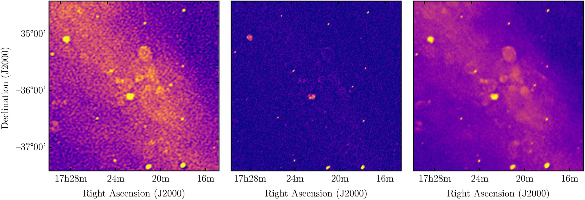
Figure 6. A region of sky centred on $\text{RA}\, 17^{\rm h}22^{\rm m}$
,
$\text{RA}\, 17^{\rm h}22^{\rm m}$
, $\text{Dec} -36^\circ$
at 139–170 MHz is shown using three different data sets and imaging techniques. Left: A single 2-min snapshot from the original Phase I configuration, imaged with multiscale WSCLean and a Briggs weighting of minus;1 (Hurley-Walker et al. Reference Hurley-Walker2019 c); Middle: A single 2-min snapshot from the extended array, imaged with multiscale WSClean and a Briggs weighting of 0; Right: The two observations imaged together using image-domain-gridding (van der Tol et al. Reference van der Tol, Veenboer and Offringa2018) in WSClean and a Briggs weighting of 0. Known SNRs are shown with solid lines, while SNRs detected by Hurley-Walker et al. (Reference Hurley-Walker2019b) are shown with dotted lines. The increased resolution and imaging quality of Phase II MWA make it possible to discern these SNRs in 4 min, instead of
$\text{Dec} -36^\circ$
at 139–170 MHz is shown using three different data sets and imaging techniques. Left: A single 2-min snapshot from the original Phase I configuration, imaged with multiscale WSCLean and a Briggs weighting of minus;1 (Hurley-Walker et al. Reference Hurley-Walker2019 c); Middle: A single 2-min snapshot from the extended array, imaged with multiscale WSClean and a Briggs weighting of 0; Right: The two observations imaged together using image-domain-gridding (van der Tol et al. Reference van der Tol, Veenboer and Offringa2018) in WSClean and a Briggs weighting of 0. Known SNRs are shown with solid lines, while SNRs detected by Hurley-Walker et al. (Reference Hurley-Walker2019b) are shown with dotted lines. The increased resolution and imaging quality of Phase II MWA make it possible to discern these SNRs in 4 min, instead of $\approx\!30$
min.
$\approx\!30$
min.
4.2. Nearby galaxies and Magellanic Clouds
Galaxy evolution is mainly governed by the combination of physical processes within the galaxy’s interstellar medium (ISM), and interactions between the galaxy and its local environment (e.g. Dickey et al. Reference Dickey, Gibson, Gomez, Imai, Jones, McClure-Griffiths, Stanimirović, van Loon, Kothes, Landecker and Willis2010). The MWA Phase II will enable significant progress within the field of galaxy evolution through integrated low-frequency synchrotron spectra studies of many more SFGs and active galactic nuclei (AGN) than was previously possible due to the order of magnitude lower noise floor compared with MWA Phase I. The low-frequency radio properties of low-redshift SFGs, for which much multi-wavelength data are available, will now be accessible through direct detections and stacking techniques.
Resolved radio observations of galactic disks, in combination with observations at other wavelengths such as the far-infrared, relate the ISM process of star formation to the magnetic fields that generate the observed radio emission observed at low frequencies (e.g. Schleicher & Beck Reference Schleicher and Beck2016; Hughes et al. Reference Hughes, Wong, Ekers, Staveley-Smith, Filipovic, Maddison, Fukui and Mizuno2006; Leverenz & Filipović Reference Leverenz and Filipović2013). Klein et al. (Reference Klein, Lisenfeld and Verley2018) show that the synchrotron spectra of nearby SFGs are not well-represented by a simple power law extending from MHz to GHz frequencies. Rather, the synchrotron spectrum at low frequencies (below 1 GHz) is rather flat, with a spectral index ( $\alpha$
where
$\alpha$
where $S_{\nu} \propto \nu^{\alpha}$
) of approximately
$S_{\nu} \propto \nu^{\alpha}$
) of approximately $-0.6$
, coupled with a break and an exponential decline at GHz frequencies. Previous studies show that the MWA Phase I synthesised beam is too large to allow for resolved radio spectral index maps of specific star-forming regions even in the nearest galaxies, such as the Magellanic Clouds (For et al. Reference For2018) and NGC 253 (Kapińska et al. Reference Kapińska2017).
$-0.6$
, coupled with a break and an exponential decline at GHz frequencies. Previous studies show that the MWA Phase I synthesised beam is too large to allow for resolved radio spectral index maps of specific star-forming regions even in the nearest galaxies, such as the Magellanic Clouds (For et al. Reference For2018) and NGC 253 (Kapińska et al. Reference Kapińska2017).
In the neighbouring Magellanic Clouds, the MWA Phase II capabilities will enable the quantification of the cosmic ray energy spectrum and the measurement of spatial variations that arise from shock re-acceleration, spectral aging, and absorption effects—the primary goal of The Deep Survey of the Magellanic System (MAGE-X, For et al. Reference For2018). The importance of hydrodynamical environmental processes such as ram pressure is understood in the cluster environment (e.g. Kenney et al. Reference Kenney, van Gorkom and Vollmer2004) as well as galaxy groups with known hot IGM (observed in X-rays; e.g. Rasmussen et al. Reference Rasmussen, Ponman and Mulchaey2006). Murphy et al. (Reference Murphy, Kenney, Helou, Chung and Howell2009) also suggest that the intracluster wind can sweep the cosmic ray electrons and associate magnetic fields to one side, creating synchrotron tails. However, the importance of these processes in low-density environments such as galaxy groups is less clear. Recent studies suggest that ram pressure may be occurring in lower-density galaxy groups without hot observable X-ray halos (Westmeier et al. Reference Westmeier, Koribalski and Braun2013). Ram pressure could also explain some of the extended radio halos that are observed in some but not all galaxies (e.g. Heesen et al. Reference Heesen2018). The role of ram pressure can be directly confirmed through the detection of synchrotron emission from a high Mach number shock at the eastern boundary of the Large Magellanic Cloud through the MAGE-X project.
Within the Magellanic Clouds, the combination of Phase II observations and soft X-ray emission (from the forthcoming eROSITA mission) will enable the investigation of the SNR population and the host ISM within the Clouds through detailed and global studies of Magellanic Cloud SNRs and superbubbles (Maggi et al. Reference Maggi2016; Kavanagh et al. Reference Kavanagh2019). Resolved analyses from the MAGE-X project are complemented by multiwavelength ancillary observations that include high-frequency radio observations (Kim et al. Reference Kim, Staveley-Smith, Dopita, Sault, Freeman, Lee and Chu2003; Hughes et al. Reference Hughes, Staveley-Smith, Kim, Wolleben and Filipović2007; Wong et al. Reference Wong2012, Reference Wong2011b; Crawford et al. Reference Crawford, Filipovic, de Horta, Wong, Tothill, Draskovic, Collier and Galvin2011; Wong et al. Reference Wong, Filipovic, Crawford, de Horta, Galvin, Draskovic and Payne2011a) in addition to forthcoming HI and continuum observations from the Galactic Australian Square Kilometre Array Pathfinder (GASKAP; Dickey et al. Reference Dickey2013) and Evolutionary Map of the Universe (EMU; (Bernal et al. Reference Bernal, Raccanelli, Kovetz, Parkinson, Norris, Danforth and Schmitt2019)) surveys using ASKAP; the mid- and far-infrared observations from Spitzer (Surveying the Agents of Galaxy Evolution minus;SAGE; Meixner et al. Reference Meixner2006) and Herschel (The HERschel Inventory of The Agents of Galaxy Evolution minus;HERITAGE; Meixner et al. Reference Meixner2013); and near-infrared observations from the ongoing VISTA survey (Cioni et al. Reference Cioni2013; Ivanov et al. Reference Ivanov2016). The Phase II observations will also have comparable angular resolution to large area optical narrow-band surveys, such as the Southern H-Alpha Sky Survey Atlas (SHASSA; Gaustad et al. Reference Gaustad, McCullough, Rosing and Van Buren2001) or the Magellanic Cloud Emission Line Survey (MCELS; Pellegrini et al. Reference Pellegrini, Oey, Winkler, Points, Smith, Jaskot and Zastrow2012) in H $\alpha$
. Such H
$\alpha$
. Such H $\alpha$
observations can be used to separate the thermal from the nonthermal components of the observed radio continuum observations (e.g. Tabatabaei et al. Reference Tabatabaei, Beck, Krügel, Krause, Berkhuijsen, Gordon and Menten2007). The resulting thermal and nonthermal radio continuum maps can be used to derive ISM physical parameters, such as magnetic field strength and thermal electron density of warm ionised gas.
$\alpha$
observations can be used to separate the thermal from the nonthermal components of the observed radio continuum observations (e.g. Tabatabaei et al. Reference Tabatabaei, Beck, Krügel, Krause, Berkhuijsen, Gordon and Menten2007). The resulting thermal and nonthermal radio continuum maps can be used to derive ISM physical parameters, such as magnetic field strength and thermal electron density of warm ionised gas.
Stellar winds and supernovae give rise to bubbles (De Horta et al. Reference De Horta2014) and superbubbles (Kavanagh et al. Reference Kavanagh, Sasaki, Bozzetto, Filipović, Points, Maggi and Haberl2015). The expansion of superbubbles is responsible for the compression and fragmentation of cool gas, and is well-traced by observations of HI, dust, and molecules (Sano et al. Reference Sano2017). Such winds may also create chimneys which bridge a galaxy’s star-forming disk and halo, facilitating the propagation of cosmic rays towards the halo via the magnetic fields in these chimneys (Norman & Ikeuchi Reference Norman and Ikeuchi1989). The abundance of extended radio halos, which are observed in a few nearby galaxies (e.g. Duric et al. Reference Duric, Irwin and Bloemen1998; Kepley et al. Reference Kepley, Mühle, Everett, Zweibel, Wilcots and Klein2010; Srivastava et al. Reference Srivastava, Kantharia, Basu, Srivastava and Ananthakrishnan2014; Kapińska et al. Reference Kapińska2017; Krause et al. Reference Krause2018), is not well understood. Significant progress in this area will also further our understanding of the connection between the galactic disk and the halo—currently one of the most active areas of investigation (e.g. Bland-Hawthorn et al. Reference Bland-Hawthorn, Maloney, Stephens, Zovaro and Popping2017). A more exotic theoretical model suggests that the observed excess of radio continuum emission in the halo of NGC 1569 may be due to dark matter annihilation (Ho et al. Reference Ho2018). Therefore, the new observations, with improved sensitivity and resolution, from the MWA Phase II will significantly further our understanding of the resolved ISM processes that connect the galactic disks to halos, as well as provide vital constraints to theoretical models.
4.3. Spectroscopy
One of the unexpected results from Phase I of the MWA is the first detections of molecules below 700 MHz (Tremblay et al. Reference Tremblay, Hurley-Walker, Cunningham, Jones, Hancock, Wayth and Jordan2017; Tremblay et al. Reference Tingay, Tremblay and Croft2018a). Tremblay et al. (Reference Tingay2018b) also made tentative detections of carbon radio recombination lines around 106 MHz. However, Phase II allows for better detection due to the reduced beam size which decreases the beam dilution. A standard assumption when determining the column density or total intensity of the emission is that the source fills the telescope’s synthesised beam. With a 2–3 arcminute beam in the surveys done with Phase I, stellar sources at 400 pc or greater distances are likely significantly smaller than the beam, creating an error in the measurements. With the longer baselines from Phase II, the beam size decreases to about 1 arcminute, allowing for better detection of weak signals and signals from greater distances. A future upgrade to the correlator will greatly improve the frequency resolution and therefore the sensitivity for currently unresolved spectral lines, further enhancing study of the kinematics and physical properties of interstellar gas for a vast range of astronomical objects.
LOFAR (van Haarlem et al. Reference van Haarlem2013) has been the current leader in the study and analysis of low-frequency carbon recombination lines with studies of Cassiopeia A (Asgekar et al. Reference Asgekar, Oonk, Yatawatta, van Weeren and McKean2013; Salas et al. Reference Salas, Oonk, van Weeren, Salgado and Morabito2017), Cygnus A (Oonk et al. Reference Oonk2014), and the extragalactic detection in M82 (Morabito et al. Reference Morabito2014). Recently, Salgado et al. (Reference Salgado, Morabito, Oonk, Salas, Toribio, Röttgering and Tielens2017a,b) published two in-depth papers on the full theoretical analysis of carbon recombination lines at the quantum states of n–bound states $>$
200 including the level population determination (influencing the strength of the detected lines) in order to develop carbon recombination lines as tools to study the physical conditions of the local gas. Following on from the work using LOFAR in the northern hemisphere, the MWA can equivalently view the low-frequency sky from the southern hemisphere. However, no other telescope has reported molecular line detections below 700 MHz.
$>$
200 including the level population determination (influencing the strength of the detected lines) in order to develop carbon recombination lines as tools to study the physical conditions of the local gas. Following on from the work using LOFAR in the northern hemisphere, the MWA can equivalently view the low-frequency sky from the southern hemisphere. However, no other telescope has reported molecular line detections below 700 MHz.
There is a range of science cases for studying astronomical phenomena in molecular and atomic spectral lines at low frequencies: high-mass star formation (Codella et al. Reference Codella2015), detection of complex organics to look for signs of life in stars and planets (Danilovich et al. Reference Danilovich, De Beck, Black, Olofsson and Justtanont2016), reviving investigation of the disproportionate ratio of organic and inorganic molecules (Cosmovici et al. Reference Cosmovici, Olthof, Strafella, Barbieri, Canton and D’Anna1979), and determining the physical properties of the ISM (Salgado et al. Reference Salgado, Morabito, Oonk, Salas, Toribio, Röttgering and Tielens2017b), including its cold diffused component (Oonk et al. Reference Oonk, Morabito, Salgado, Toribio, van Weeren, Tielens and Rottgering2015; Peters et al. Reference Peters, Lazio, Clarke, Erickson and Kassim2011). The study of molecules around high-mass stars is complicated partially due to strong emission of prominent molecules which would not be present at lower radio frequencies. In addition, spectroscopic capability at low frequencies offers the opportunity to search for highly redshifted (z > 5) neutral hydrogen absorption towards radio AGN in the early Universe (e.g. Bañados et al. Reference Bañados, Carilli, Walter, Momjian, Decarli, Farina, Mazzucchelli and Venemans2018), and hydrogen recombination line masers from the EoR (Spaans & Norman Reference Spaans and Norman1997). Detections will enable a unique investigation of the physical conditions of the intergalactic medium at the end of the EoR and the cold gas feeding massive galaxy formation in the early Universe.
4.4. The cosmic web and galaxy clusters
4.4.1. The synchrotron cosmic web
The large-scale structure of the Universe requires the presence of intergalactic shocks, which are in turn expected to accelerate electrons and amplify intergalactic magnetic fields (Keshet et al. Reference Keshet, Waxman and Loeb2004b; Brüggen et al. Reference Brüggen, Ruszkowski, Simionescu, Hoeft and Dalla Vecchia2005; Hoeft & Brüggen Reference Hoeft and Brüggen2007; Battaglia et al. Reference Battaglia, Pfrommer, Sievers, Bond and Enßlin2009; Araya-Melo et al. Reference Araya-Melo, Aragón-Calvo, Brüggen and Hoeft2012). These shocks should thus produce faint synchrotron emission, which can act as a tracer of large-scale structure, cosmic filaments, and primordial magnetic fields (Keshet et al. Reference Keshet, Waxman and Loeb2004a; Wilcots Reference Wilcots2004; Donnert et al. Reference Donnert, Dolag, Lesch and Müller2009; Vazza et al. Reference Vazza, Ferrari, Bonafede, Brüggen, Gheller, Braun and Brown2015a,b; Brown et al. Reference Brown2017b). Detection of this ‘synchrotron cosmic web’ can provide a direct image of the large-scale structure of the Universe, act as a laboratory for studying particle acceleration in low-density shocks, lead to a measurement of the magnetic field strength of the intergalactic medium, and provide a direct discriminant on competing models for the origin of cosmic magnetism. It is predicted that the signal from the synchrotron cosmic web should dominate other radio signals on scales of $\sim10'$
to
$\sim10'$
to $\sim1^\circ$
at frequencies around 100 MHz (Keshet et al. Reference Keshet, Waxman and Loeb2004b; Vazza et al. Reference Vazza, Ferrari, Bonafede, Brüggen, Gheller, Braun and Brown2015a), making the MWA a well-suited facility to search for these structures.
$\sim1^\circ$
at frequencies around 100 MHz (Keshet et al. Reference Keshet, Waxman and Loeb2004b; Vazza et al. Reference Vazza, Ferrari, Bonafede, Brüggen, Gheller, Braun and Brown2015a), making the MWA a well-suited facility to search for these structures.
Vernstrom et al. (Reference Vernstrom, Gaensler, Brown, Lenc and Norris2017) have carried out a search for the synchrotron cosmic web with the Phase I MWA, in which they cross-correlated diffuse radio emission imaged at 180 MHz with large-scale structure traced by infrared galaxy surveys. They were able to place upper limits on the surface brightness of the synchrotron cosmic web of $0.01\,-\,0.3\text{mJy\,arcmin}^{-2}$
, which translates to upper limits on the magnetic field strength of 0.03 – 1.98
$0.01\,-\,0.3\text{mJy\,arcmin}^{-2}$
, which translates to upper limits on the magnetic field strength of 0.03 – 1.98
 $${\rm{\mu }}$$
G, assuming equipartition. While these constraints are not yet deep enough to differentiate between different cosmic magnetism models, the limits are comparable to other limits from cluster observations (e.g. Feretti et al. Reference Feretti, Perley, Giovannini and Andernach1999; Brunetti et al. Reference Brunetti, Setti, Feretti and Giovannini2001; Brown et al. Reference Brown, Farnsworth and Rudnick2010) or predictions from MHD simulations (e.g. Donnert et al. Reference Donnert, Dolag, Lesch and Müller2009; Vazza et al. Reference Vazza, Ferrari, Brüggen, Bonafede, Gheller and Wang2015b).
$${\rm{\mu }}$$
G, assuming equipartition. While these constraints are not yet deep enough to differentiate between different cosmic magnetism models, the limits are comparable to other limits from cluster observations (e.g. Feretti et al. Reference Feretti, Perley, Giovannini and Andernach1999; Brunetti et al. Reference Brunetti, Setti, Feretti and Giovannini2001; Brown et al. Reference Brown, Farnsworth and Rudnick2010) or predictions from MHD simulations (e.g. Donnert et al. Reference Donnert, Dolag, Lesch and Müller2009; Vazza et al. Reference Vazza, Ferrari, Brüggen, Bonafede, Gheller and Wang2015b).
The depth of the search reported by Vernstrom et al. (Reference Vernstrom, Gaensler, Brown, Lenc and Norris2017) was limited by confusion, in that large numbers of unresolved extragalactic radio sources have not been subtracted from the data, and may mimic diffuse radio emission that traces large-scale structure. As for many other continuum science programs, the improved angular resolution and reduced confusion levels offered by MWA Phase II will enable much deeper searches for the synchrotron cosmic web, whether by direct imaging (e.g. Kronberg et al. Reference Kronberg, Kothes, Salter and Perillat2007), statistical cross-correlations (Vernstrom et al. Reference Vernstrom, Gaensler, Brown, Lenc and Norris2017; Brown et al. Reference Brown2017b), or also in polarimetry (Rudnick & Brown Reference Rudnick and Brown2009; Brown et al. Reference Brown, Rudnick, Farnsworth, Strassmeier, Kosovichev and Beckman2009).
4.4.2. Diffuse emission in galaxy clusters
In addition to the potential detection of the large-scale, diffuse emission predicted by the cosmic web, the Phase I MWA has proven itself to be a powerful instrument for the detection and study of diffuse, low-surface brightness emission in galaxy clusters.
Diffuse emission in clusters manifests in a variety of forms including central radio halos, which are believed to be the result of turbulence in the cluster core; mini-halos powered by central AGN; peripheral radio relics which result from strong shocks generated in cluster mergers; and radio phoenices which trace the passage of these shocks across the lobes of AGN (see Kempner et al. (Reference Kempner, Blanton, Clarke, Enßlin, Johnston-Hollitt, Rudnick, Reiprich, Kempner and Soker2004) for the taxonomy of cluster sources and Brunetti & Jones (Reference Brunetti and Jones2014) for a review of the physics of emission in galaxy clusters). Recently, Govoni et al. (Reference Govoni2019) observed diffuse emission at 140 MHz connecting the clusters Abell 0399 and Abell 0401 with LOFAR.
Although on different physical scales from hundreds of kpc (mini-halos and phoenices) to Mpc-scale (halos and relics), one defining characteristic of these sources is their steep radio spectral indices. In the case of halos, the average spectral index is $-1.3$
, with some examples with spectral indices steeper than
$-1.3$
, with some examples with spectral indices steeper than $-2$
being detected in MWA data (Duchesne et al. Reference Duchesne, Johnston-Hollitt, Offringa, Pratt, Zheng and Dehghan2017). Such emission characteristics make the detection of diffuse cluster emission considerably easier at low frequencies and the large physical scales make detection easier with instruments sensitive to angular scales of the order of arcminutes. The MWA is thus ideal, and a large number of new and existing sources of diffuse emission in clusters and groups have already been detected and studied with the Phase I array (Hindson et al. Reference Hindson2014; Schellenberger et al. Reference Schellenberger, Vrtilek, David, O’Sullivan, Giacintucci, Johnston-Hollitt, Duchesne and Raychaudhury2017; Duchesne et al. Reference Duchesne, Johnston-Hollitt, Offringa, Pratt, Zheng and Dehghan2017).
$-2$
being detected in MWA data (Duchesne et al. Reference Duchesne, Johnston-Hollitt, Offringa, Pratt, Zheng and Dehghan2017). Such emission characteristics make the detection of diffuse cluster emission considerably easier at low frequencies and the large physical scales make detection easier with instruments sensitive to angular scales of the order of arcminutes. The MWA is thus ideal, and a large number of new and existing sources of diffuse emission in clusters and groups have already been detected and studied with the Phase I array (Hindson et al. Reference Hindson2014; Schellenberger et al. Reference Schellenberger, Vrtilek, David, O’Sullivan, Giacintucci, Johnston-Hollitt, Duchesne and Raychaudhury2017; Duchesne et al. Reference Duchesne, Johnston-Hollitt, Offringa, Pratt, Zheng and Dehghan2017).
A particular strength of the MWA is the ability to perform detailed spectral studies of these sources across the MWA band. Figure 7 shows the in-band spectral measurements and resultant fit for the source complex extended cluster source NGC 741 taken from the MWA’s GLEAM survey (Wayth et al. Reference Wayth2015). This plot demonstrates the extremely fine spectral resolution of the MWA as compared to existing arrays (for a full analysis of these data, see Schellenberger et al. Reference Schellenberger, Vrtilek, David, O’Sullivan, Giacintucci, Johnston-Hollitt, Duchesne and Raychaudhury2017). Having such high-fidelity spectral information has been invaluable in constraining the physical processes at work to generate the emission, allowing separation of sources that would otherwise be morphologically indistinct into classes based on the underlying acceleration mechanisms and age of the electron population (Schellenberger et al. Reference Schellenberger, Vrtilek, David, O’Sullivan, Giacintucci, Johnston-Hollitt, Duchesne and Raychaudhury2017).
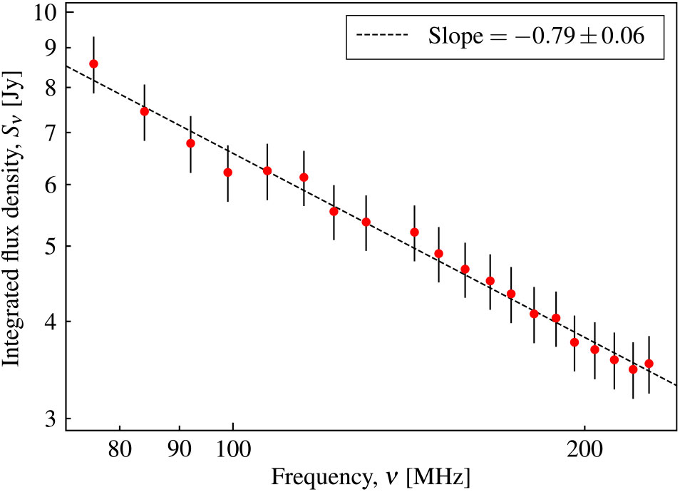
Figure 7. MWA data for the complex cluster source NGC 741, showing the unprecedented ability of the MWA to determine spectral indices across the MWA band. Further information and analysis of these data are available in Schellenberger et al. (Reference Schellenberger, Vrtilek, David, O’Sullivan, Giacintucci, Johnston-Hollitt, Duchesne and Raychaudhury2017).
4.5. AGN and star-forming galaxies
The population of radio continuum sources is dominated by radio-loud AGN at bright fluxes with an increasing fraction of star-forming galaxies (SFGs) as radio surveys reach lower sensitivities (Seymour et al. Reference Seymour, McHardy and Gunn2004). Consequently, the first extragalactic data release of GLEAM (Hurley-Walker et al. Reference Hurley-Walker2017) contains mostly radio-loud AGN with only a few local SFGs detected. The wide area of GLEAM and the broadband radio SEDs have allowed unique classifications of radio sources by their SEDs (Harvey et al. Reference Harvey, Franzen, Morgan and Seymour2018). Detailed studies of radio-loud AGN (Herzog et al. Reference Herzog2016; Callingham et al. Reference Callingham2017) and local powerful SFGs (Kapińska et al. Reference Kapińska2017; Galvin et al. Reference Galvin2018) are therefore possible. However, the depth of GLEAM was limited by the confusion limit from the 3 km baselines. With MWA Phase II, the confusion limit drops by over an order of magnitude allowing far deeper surveys to be conducted.
4.5.1. AGN evolution
The long baselines have allowed us to conduct new broad-frequency continuum surveys: the eXtended GLEAM survey (GLEAM-X) and the MWA Interestingly Deep Astrophysical (MIDAS) survey. GLEAM-X is a repeat of the all-sky GLEAM, but with longer total integration in addition to the higher resolution (reaching more than $\sim\! 5\times$
the depth of GLEAM). MIDAS is going at least twice as deep as GLEAM-X, targeting six well-studied extragalactic fields: the five Galaxy And Mass Assembly (GAMA) survey fields (Driver et al. Reference Driver2009) and the Spitzer South Pole Telescope Deep Field (Ashby et al. Reference Ashby2014). The GAMA survey fields cover
$\sim\! 5\times$
the depth of GLEAM). MIDAS is going at least twice as deep as GLEAM-X, targeting six well-studied extragalactic fields: the five Galaxy And Mass Assembly (GAMA) survey fields (Driver et al. Reference Driver2009) and the Spitzer South Pole Telescope Deep Field (Ashby et al. Reference Ashby2014). The GAMA survey fields cover $250 \text{deg}^{2}$
with exquisite photometry from UV to the far-IR. These fields also include spectroscopic redshifts, group catalogues, and derived data products such as stellar mass and star formation rate. The fusion of these data sets will allow a plethora of science including determining the luminosity function, and the nature and evolution of the low-frequency selected radio population.
$250 \text{deg}^{2}$
with exquisite photometry from UV to the far-IR. These fields also include spectroscopic redshifts, group catalogues, and derived data products such as stellar mass and star formation rate. The fusion of these data sets will allow a plethora of science including determining the luminosity function, and the nature and evolution of the low-frequency selected radio population.
In concert with deep ongoing surveys from ASKAP (Norris et al. Reference Norris2011), uGMRT (Swarup et al. Reference Swarup, Ananthakrishnan, Kapahi, Rao, Subrahmanya and Kulkarni1991), and the Australia Telescope Compact Array (ATCA; GAMA Legacy ATCA Southern Survey minus;GLASS) MWA observations will yield broadband SEDs for tens of thousands of sources in the GAMA fields. A large fraction of these will have spectroscopic redshifts and derived host galaxies properties. This unique data set will provide estimates of jet powers for these radio-loud AGN which can be compared to other processes such as accretion rate and star formation (e.g. Gürkan et al. Reference Gürkan2018).
The improvement in sensitivity is also beneficial to the study of Giant Radio Galaxies (GRGs), which are AGN with emission that extends over $\sim$
700 kpc. Fine details of this extended emission can now be resolved with the addition of the long baselines, allowing for studies of spectral properties such as the spectral ageing of the lobes, enabling detailed modelling of source environments. As an example, Figure 8 compares images of the giant radio galaxy ESO 422 minus;G028 using Phase I and Phase II data. The Phase II data were imaged using robust
$\sim$
700 kpc. Fine details of this extended emission can now be resolved with the addition of the long baselines, allowing for studies of spectral properties such as the spectral ageing of the lobes, enabling detailed modelling of source environments. As an example, Figure 8 compares images of the giant radio galaxy ESO 422 minus;G028 using Phase I and Phase II data. The Phase II data were imaged using robust $=+1.0$
to improve sensitivity to ultra-diffuse large-scale emission from this GRG. The improvement in sensitivity and resolution offered by Phase II of the MWA is illustrated by the ultra-faint diffuse emission from the tails of ESO 422 recovered at much greater significance compared to Phase I. With the factor
$=+1.0$
to improve sensitivity to ultra-diffuse large-scale emission from this GRG. The improvement in sensitivity and resolution offered by Phase II of the MWA is illustrated by the ultra-faint diffuse emission from the tails of ESO 422 recovered at much greater significance compared to Phase I. With the factor $\sim\!2-3$
improvement in resolution offered by Phase II, such data can be used in conjunction with higher-frequency data from other cutting edge radio telescopes (e.g. uGMRT, ASKAP, and the ATCA) to probe the spectral properties of extended radio galaxies at much improved angular resolution compared to Phase I.
$\sim\!2-3$
improvement in resolution offered by Phase II, such data can be used in conjunction with higher-frequency data from other cutting edge radio telescopes (e.g. uGMRT, ASKAP, and the ATCA) to probe the spectral properties of extended radio galaxies at much improved angular resolution compared to Phase I.
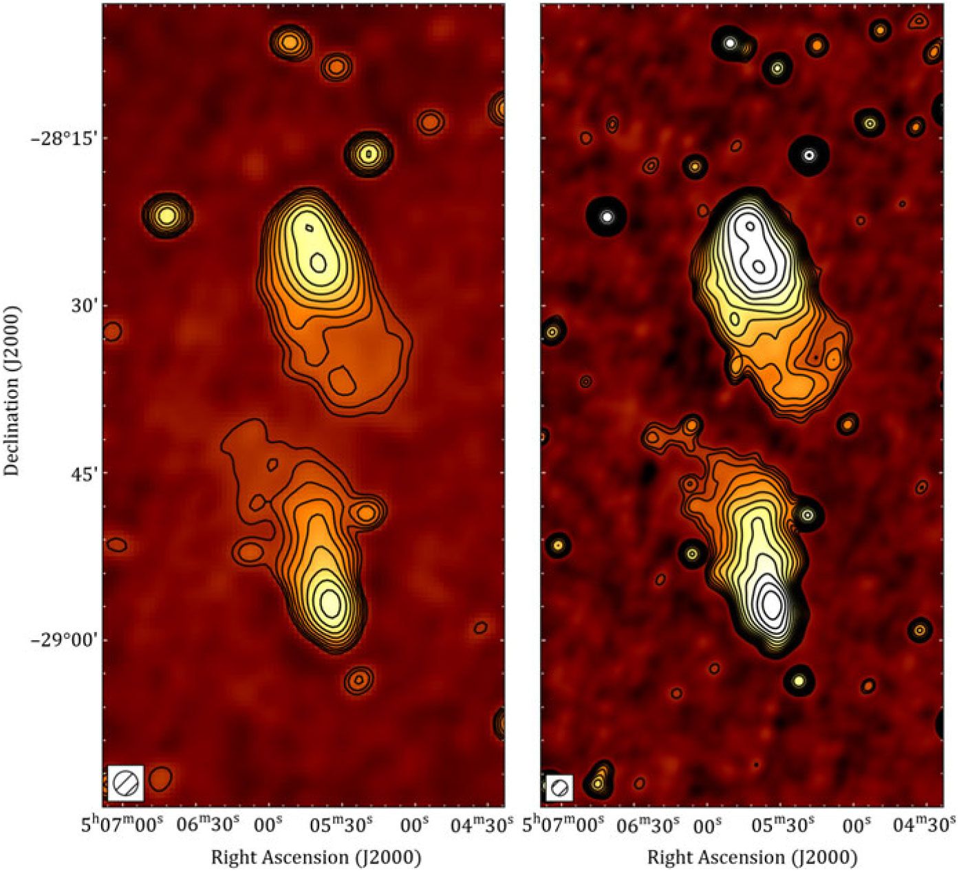
Figure 8. Images of ESO 422 minus;G028 from Phase I (left, from GLEAM; Hurley-Walker et al. (Reference Hurley-Walker2017)) and Phase II (right, from GLEAM-X). Colour-scale and contours both denote the surface brightness at 200 MHz. Colour scale ranges from $-3$
to
$-3$
to $100\sigma$
on an arcsinh stretch to emphasise faint diffuse emission. Contours start at
$100\sigma$
on an arcsinh stretch to emphasise faint diffuse emission. Contours start at $3\sigma$
and scale by a factor
$3\sigma$
and scale by a factor $\sqrt{2}$
, where
$\sqrt{2}$
, where $\sigma=14.9 \text{mJy beam}^{-1}$
(
$\sigma=14.9 \text{mJy beam}^{-1}$
( $2.0 \text{mJy beam}^{-1}$
) in the Phase I (Phase II) image. The beam size is shown by the hatched ellipse in the lower-left corner.
$2.0 \text{mJy beam}^{-1}$
) in the Phase I (Phase II) image. The beam size is shown by the hatched ellipse in the lower-left corner.
4.5.2. Powerful AGN
The GLEAM 4-Jy Sample (White et al. Reference White2018), selected at 151 MHz, contains 1 863 bright radio sources and is dominated by AGN. This includes 77 radio galaxies that are so extended that they are resolved into multiple GLEAM components by the MWA Phase I beam. However, approximately one-fifth of the sample suffers from confusion which will be alleviated by higher resolution allowing them to be more easily classified and cross-matched. The 4-Jy sample will be a benchmark for the bright radio galaxy population, like 3CRR (Laing et al. Reference Laing, Riley and Longair2003), but is an order of magnitude larger.
GLEAM has also allowed us to search for powerful very high-redshift sources through a number of techniques including ultra-steep spectrum, curved SED, and compactness (from IPS, see Section 6.2.1). This ongoing work to obtain their redshifts is proving fruitful with follow-up on 8 m class telescopes and with the Atacama Large Millimetre Array (e.g. Seymour Reference Seymour2019).
4.6. Star-forming galaxies
While SFGs are rare in GLEAM, one of the dramatic results to come out of their study was the fact that their SEDs are more complex than had generally been appreciated with flattening and even turnovers at low frequency as well as kinks at high frequency (Kapińska et al. Reference Kapińska2017; Galvin et al. Reference Galvin2018). These features are thought to be due to multiple star-forming components, and free–free absorption. Understanding how this complexity is related to the underlying star formation is important as using deep radio surveys to trace the star formation history of the Universe is key science goal of the SKA (Braun et al. Reference Braun, Bourke, Green, Keane and Wagg2015).
4.6.1. Compact steep spectrum and gigahertz-peaked spectrum radio sources
Compact steep spectrum (CSS) and gigahertz-peaked spectrum (GPS) radio sources are a class of compact radio-loud AGN that are thought to be the young precursors to large-scale radio galaxies (O’Dea Reference O’Dea1998). The lower radio luminosity ( $< 10^{25}\text{ W/Hz}$
at 5 GHz) sample of GPS and CSS sources has been suggested to be dominated by the objects strongly affected during their evolution by an interaction with the ISM or instability in the accretion disk (Czerny et al. Reference Czerny, Siemiginowska, Janiuk, Nikiel-Wroczyński and Stawarz2009; Bicknell et al. Reference Bicknell, Mukherjee, Wagner, Sutherland and Nesvadba2018). Such sources could be the short-lived precursors needed to account for the overabundance of GPS and CSS sources relative to the large-scale radio galaxies (Kunert-Bajraszewska et al. Reference Kunert-Bajraszewska, Gawroński, Labiano and Siemiginowska2010). However, none of the low-luminosity peaked-spectrum samples to date have been large enough, or devoid of selection biases, to justify this conclusion. The increased sensitivity of MWA Phase II will be able to probe a significantly fainter population of peaked-spectrum sources than previously possible (Callingham et al. Reference Callingham2017). While other telescopes such as LOFAR have the required sensitivity to access the low-luminosity peaked-spectrum population, LOFAR currently lacks the wide fractional bandwidth needed to identify peaked-spectrum candidates nontrivially when solely using LOFAR data. Therefore, the large fractional bandwidth of the MWA, combined with the high sensitivity of Phase II, represents a significant advantage for this science.
$< 10^{25}\text{ W/Hz}$
at 5 GHz) sample of GPS and CSS sources has been suggested to be dominated by the objects strongly affected during their evolution by an interaction with the ISM or instability in the accretion disk (Czerny et al. Reference Czerny, Siemiginowska, Janiuk, Nikiel-Wroczyński and Stawarz2009; Bicknell et al. Reference Bicknell, Mukherjee, Wagner, Sutherland and Nesvadba2018). Such sources could be the short-lived precursors needed to account for the overabundance of GPS and CSS sources relative to the large-scale radio galaxies (Kunert-Bajraszewska et al. Reference Kunert-Bajraszewska, Gawroński, Labiano and Siemiginowska2010). However, none of the low-luminosity peaked-spectrum samples to date have been large enough, or devoid of selection biases, to justify this conclusion. The increased sensitivity of MWA Phase II will be able to probe a significantly fainter population of peaked-spectrum sources than previously possible (Callingham et al. Reference Callingham2017). While other telescopes such as LOFAR have the required sensitivity to access the low-luminosity peaked-spectrum population, LOFAR currently lacks the wide fractional bandwidth needed to identify peaked-spectrum candidates nontrivially when solely using LOFAR data. Therefore, the large fractional bandwidth of the MWA, combined with the high sensitivity of Phase II, represents a significant advantage for this science.
4.6.2. Dying radio galaxies
As with the diffuse emission in galaxy clusters, the MWA has a niche capability in the detection of diffuse, low surface brightness emission from the lobes of old, dead, or dying radio galaxies. One such early example was the detection of previously unknown giant radio lobes associated with the lenticular galaxy NGC 1534 (Hurley-Walker et al. Reference Hurley-Walker2015; Duchesne & Johnston-Hollitt Reference Duchesne and Johnston-Hollitt2018). Work in this field across a range of low-frequency telescopes has seen the detection of several more such sources, suggesting a significant and previously unknown population of sources (e.g. de Gasperin et al. Reference de Gasperin, Intema, Williams, Brüggen, Murgia, Beck and Bonafede2014; Brienza et al. Reference Brienza2016; Mahatma et al. Reference Mahatma2018). However, as with the diffuse emission in galaxy clusters, the volume over which remnant or dying radio galaxies can be detected was limited with the Phase I array to the very local Universe. If we assume a typical size for such sources of 700 kpc, in order to resolve the lobes of such galaxies, the Phase I MWA would have been limited to sources with redshifts less than 0.17. Even detecting such sources in the nearby Universe, the Phase I MWA had insufficient resolution to perform spectral imaging across the lobes of the radio sources, which is vital to understanding the physics of such sources. As a result while the Phase I MWA was able to detect some of this class of object, no detailed imaging could be undertaken. The detection limits with the Phase II array can be pushed out to redshifts of z $\sim$
0.42, which considerably expands the volume in which such sources can be found. Furthermore, there will be sufficient resolution to perform detailed statistical spectral studies over the radio lobes of nearby sources, which is vital to understand the physics of such systems.
$\sim$
0.42, which considerably expands the volume in which such sources can be found. Furthermore, there will be sufficient resolution to perform detailed statistical spectral studies over the radio lobes of nearby sources, which is vital to understand the physics of such systems.
4.7. Polarimetry
The detection and characterisation of polarised sources in the low-frequency sky is a challenging endeavour due to the Faraday depolarisation of radio sources with increasing wavelength. This is further compounded in the case of low-resolution instruments where beam depolarisation can occur. Nevertheless, polarimetry campaigns are ongoing across a number of low-frequency instruments including LOFAR, PAPER, and the upgraded GMRT (Jelić et al. Reference Jelić2014; Kohn et al. Reference Kohn2016; Van Eck et al. Reference Van Eck2018; O’Sullivan et al. Reference O’Sullivan2018a). The MWA’s wide FOV and broad frequency coverage make it a highly efficient facility for the detection of polarised radio sources, highly precise determinations of their Faraday rotation measures (RMs), and the study of Faraday complexity.
Exploration of the polarised sky with the MWA commenced with the 32-tile prototype array (Bernardi et al. Reference Bernardi2013) and has continued for both compact extragalactic (Lenc et al. Reference Lenc2017; Riseley et al. Reference Riseley2018) and diffuse, wide-field Galactic emission with the Phase I array (Lenc et al. Reference Lenc2016). The total number of discrete polarised point sources detected with the Phase I MWA was expected to be low due to limited sensitivity and angular resolution ( $\sim\!250$
linearly polarised sources estimated across the visible Southern sky; Lenc et al. Reference Lenc2017). Re-analysis of the Phase I GLEAM survey data as described by Riseley et al. (Reference Riseley2018) has proven to be an effective method of identifying and studying such sources, and has now yielded about a factor of 2 higher source density of extragalactic polarised sources than projected, in addition to 10 of pulsars detected in polarisation after targeted inspection. All of the extragalactic polarised sources are AGN. Many are detected in polarisation from the hotspots of Fanaroff–Riley type II (FRII) sources, and some are interesting multi-component cases such as PKS J0636 minus;2036, which is the first source for which a broadband polarimetric study (wavelength-squared coverage from 1.7 to
$\sim\!250$
linearly polarised sources estimated across the visible Southern sky; Lenc et al. Reference Lenc2017). Re-analysis of the Phase I GLEAM survey data as described by Riseley et al. (Reference Riseley2018) has proven to be an effective method of identifying and studying such sources, and has now yielded about a factor of 2 higher source density of extragalactic polarised sources than projected, in addition to 10 of pulsars detected in polarisation after targeted inspection. All of the extragalactic polarised sources are AGN. Many are detected in polarisation from the hotspots of Fanaroff–Riley type II (FRII) sources, and some are interesting multi-component cases such as PKS J0636 minus;2036, which is the first source for which a broadband polarimetric study (wavelength-squared coverage from 1.7 to $16\text{ m}^2$
) has been undertaken using combined MWA and ATCA imaging (O’Sullivan et al. Reference O’Sullivan, Lenc, Anderson, Gaensler and Murphy2018b). Detailed study of the Faraday complexity of polarised sources detected with the MWA is possible by combining data from ASKAP’s forthcoming Polarisation Sky Survey of the Universe’s Magnetism (POSSUM; Gaensler et al. Reference Gaensler, Landecker, Taylor and Collaboration2010) survey and the ATCA QUOCKA survey which spans the 1–8.5 GHz frequency range.
$16\text{ m}^2$
) has been undertaken using combined MWA and ATCA imaging (O’Sullivan et al. Reference O’Sullivan, Lenc, Anderson, Gaensler and Murphy2018b). Detailed study of the Faraday complexity of polarised sources detected with the MWA is possible by combining data from ASKAP’s forthcoming Polarisation Sky Survey of the Universe’s Magnetism (POSSUM; Gaensler et al. Reference Gaensler, Landecker, Taylor and Collaboration2010) survey and the ATCA QUOCKA survey which spans the 1–8.5 GHz frequency range.
The Phase II MWA is expected to detect vastly more compact polarised sources through both the reduction in beam depolarisation provided by the longer baselines and the improvement in sensitivity, particularly for imaging modes where the longest baselines are not significantly down-weighted (Lenc et al. Reference Lenc2017).
In addition, the improved resolution of the Phase II MWA will allow a more detailed exploration of the vast swaths of diffuse, linearly polarised Galactic emission detectable by the MWA (Lenc et al. Reference Lenc2016). Study of the diffuse Galactic polarised emission, together with Faraday RMs of extragalactic sources and polarised pulsars, allows holistic modelling of the three-dimensional Milky Way magnetic field. For example, RMs of pulsars embedded within the Galactic halo provide constraints on the vertical change in magnetic field strength (Sobey et al. Reference Sobey2019).
Finally, consideration of circular polarisation measurements with the Phase II MWA will detect flare stars and has the potential to make the first low-frequency detection of exoplanets. In the case of flare stars, the Phase I MWA has already verified the potential for faint flares to be detected in polarised images. Lynch et al. (Reference Lynch, Lenc, Kaplan, Murphy and Anderson2017b) detected four flares from UV Ceti with the Phase I array, each with flux densities over two orders of magnitude fainter than previously reported. Due to confusion in the total intensity imaging, these faint flares were only detectable in the polarised images, demonstrating the power of low-frequency arrays to perform such searches in circular polarisation. The improved characteristics of the Phase II MWA should thus allow for more such detections and an assessment of their temporal characteristics. Furthermore, although previous attempts to directly detect exoplanet emission with the MWA via circular polarisation have been unsuccessful, setting only upper limits (Murphy et al. Reference Murphy2015; Lynch et al. Reference Lynch, Murphy, Kaplan, Ireland and Bell2017a), the experiment should be repeated with the Phase II array which is expected to be an order of magnitude more sensitive as discussed in Section 4.4.1. We further discuss MWA exoplanet searches in the context of transient science in Section 5.4.
4.8. Complementarity with other surveys
The MWA upgrade is taking place in the context of a revolutionary period in radio astronomy, with several new large radio surveys taking place on major new or dramatically upgraded telescopes around the world, resulting in an increase by a factor of $\sim$
50 in the number of known radio sources (Norris Reference Norris2017). Of particular relevance to MWA surveys is the northern-hemisphere LOFAR Two-Metre Sky Survey (LoTSS Shimwell et al. Reference Shimwell2017), with similar frequency band (120168 MHz) and higher angular resolution (
$\sim$
50 in the number of known radio sources (Norris Reference Norris2017). Of particular relevance to MWA surveys is the northern-hemisphere LOFAR Two-Metre Sky Survey (LoTSS Shimwell et al. Reference Shimwell2017), with similar frequency band (120168 MHz) and higher angular resolution ( $\sim$
5 arcsecond). The SKA precursor continuum surveys MIGHTEE (Jarvis et al. Reference Jarvis2016) on MeerKAT (Jonas Reference Jonas2009), and EMU (Norris et al. Reference Norris2011) and POSSUM (Gaensler et al. Reference Gaensler, Landecker, Taylor and Collaboration2010) on ASKAP (Johnston et al. Reference Johnston2008) will provide higher-frequency data for MWA sources, and the VLASS survey (Murphy & VLASS Survey Science Group Reference Murphy2015; Lacy et al., Reference Lacy2019) will provide even higher frequency and high-resolution coverage over the northern half of the MWA coverage. Also important is the major upgrade of the GMRT (Gupta et al. Reference Gupta2017), which is likely to generate surveys of large parts of the sky from 150 to 1400 MHz. For total intensity studies of extragalactic source SEDs, the EMU survey on ASKAP is particularly important as it will produce a catalogue of high-frequency counterparts for all sources detected by the MWA. ASKAP can measure the SED from 700 to 1800 MHz. Because the ASKAP configuration includes many short baselines, the data can be tapered in the uv plane to match MWA resolution with only a small loss of sensitivity. Thus, images with matched resolution can be generated at 150–300 MHz with MWA, and 700–1800 MHz with ASKAP, to produce reliable SEDs from 150 to 1800 MHz with only a relatively small gap (300–700 MHz) in frequency coverage. These broadband SEDs will obviously be important for studies of clusters (see Section 4.4), but will be particularly important for studies of radio AGN. Recent studies (e.g. Callingham et al. Reference Callingham2017) have shown that a significant fraction of radio sources have curved or peaked SEDs accessible by the joint MWA/ASKAP coverage, and modelling of this is likely to lead to a good understanding of their evolutionary stage, and perhaps even redshifts.
$\sim$
5 arcsecond). The SKA precursor continuum surveys MIGHTEE (Jarvis et al. Reference Jarvis2016) on MeerKAT (Jonas Reference Jonas2009), and EMU (Norris et al. Reference Norris2011) and POSSUM (Gaensler et al. Reference Gaensler, Landecker, Taylor and Collaboration2010) on ASKAP (Johnston et al. Reference Johnston2008) will provide higher-frequency data for MWA sources, and the VLASS survey (Murphy & VLASS Survey Science Group Reference Murphy2015; Lacy et al., Reference Lacy2019) will provide even higher frequency and high-resolution coverage over the northern half of the MWA coverage. Also important is the major upgrade of the GMRT (Gupta et al. Reference Gupta2017), which is likely to generate surveys of large parts of the sky from 150 to 1400 MHz. For total intensity studies of extragalactic source SEDs, the EMU survey on ASKAP is particularly important as it will produce a catalogue of high-frequency counterparts for all sources detected by the MWA. ASKAP can measure the SED from 700 to 1800 MHz. Because the ASKAP configuration includes many short baselines, the data can be tapered in the uv plane to match MWA resolution with only a small loss of sensitivity. Thus, images with matched resolution can be generated at 150–300 MHz with MWA, and 700–1800 MHz with ASKAP, to produce reliable SEDs from 150 to 1800 MHz with only a relatively small gap (300–700 MHz) in frequency coverage. These broadband SEDs will obviously be important for studies of clusters (see Section 4.4), but will be particularly important for studies of radio AGN. Recent studies (e.g. Callingham et al. Reference Callingham2017) have shown that a significant fraction of radio sources have curved or peaked SEDs accessible by the joint MWA/ASKAP coverage, and modelling of this is likely to lead to a good understanding of their evolutionary stage, and perhaps even redshifts.
This wide frequency range will also be important for polarisation studies. Combining the polarisation data from MWA (Lenc et al. Reference Lenc2017) with that from the POSSUM project on ASKAP and the ATCA QUOCKA survey will be ideal for studying Faraday synthesis. A full understanding of the magnetic field properties of polarised sources detected with the MWA will be provided by detailed modelling of the combined polarised SEDs (see, e.g., Anderson et al. Reference Anderson, Gaensler and Feain2016; O’Sullivan et al. Reference O’Sullivan2018a). Here, most of the coverage in the relevant $\lambda^2$
domain comes from the MWA.
$\lambda^2$
domain comes from the MWA.
5. Time domain astrophysics
Many exciting astrophysics topics of the day lie in the time domain including the deluge of characterised exoplanets, the intriguing nature of FRBs, the first detections of GWs and their electromagnetic counterparts, and indeed most multi-messenger astrophysics. The MWA’s recently deployed rapid-response triggering system and new VCS buffer mode have greatly improved the telescope’s ability to react to alerts from other observatories. The high resolution of the extended configuration will enable better localisation constraints, while the higher correlator data rate enables transient follow-up at high time resolution and exploration of wider range of DMs of prompt radio signals (e.g. Sokolowski et al. Reference Sokolowski2018). On the other hand, the already wide FOV, new compact configuration, continued development of tied-array beamforming (Ord et al. Reference Ord, Tremblay, McSweeney, Bhat, Sobey, Mitchell, Hancock and Kirsten2019; Xue et al. Reference Xue, Ord, Tremblay, Bhat, Sobey, Meyers, McSweeney and Swainston2019), and the new BL back-end make the MWA an extremely powerful instrument for blind transient searches. Here, we discuss the new science afforded by these improvements.
5.1. Gamma-ray bursts
Gamma-ray bursts (GRBs) are one of the most energetic phenomena in the Universe, hallmarked by their bright flash of gamma-ray emission. GRBs are detected by dedicated satellites such as the Fermi Swift Burst Alert Telescope (Barthelmy et al. Reference Barthelmy2005) and the Fermi Fermi Gamma-ray Burst Monitor (Meegan et al. Reference Meegan2009), which transmit alerts in near-real-time that allow for rapid multi-wavelength follow-up. Short-duration gamma-ray bursts (SGRBs, which last $<\!2$
s; Kouveliotou et al. Reference Kouveliotou, Meegan, Fishman, Bhat, Briggs, Koshut, Paciesas and Pendleton1993) are of particular interest due to the recent, near-simultaneous detection of the GW event GW170817 and GRB 170817A (the latter of which was detected by Fermi Fermi; Abbott et al. Reference Abbott2017 c), which strongly supports the proposed link between binary neutron star (BNS) mergers and SGRBs (Eichler et al. Reference Eichler, Livio, Piran and Schramm1989). Detailed multi-wavelength studies of SGRBs can therefore shed light on GW afterglows by providing a template of their brightness and timing properties that will inform the follow-up of future GW events by wide-field instruments.
$<\!2$
s; Kouveliotou et al. Reference Kouveliotou, Meegan, Fishman, Bhat, Briggs, Koshut, Paciesas and Pendleton1993) are of particular interest due to the recent, near-simultaneous detection of the GW event GW170817 and GRB 170817A (the latter of which was detected by Fermi Fermi; Abbott et al. Reference Abbott2017 c), which strongly supports the proposed link between binary neutron star (BNS) mergers and SGRBs (Eichler et al. Reference Eichler, Livio, Piran and Schramm1989). Detailed multi-wavelength studies of SGRBs can therefore shed light on GW afterglows by providing a template of their brightness and timing properties that will inform the follow-up of future GW events by wide-field instruments.
GRBs afterglows, which are generated by the interactions of their relativistic jets with the surrounding medium, are also known sources of radio emission in the GHz range (Piran Reference Piran1999). However, it is unlikely that such afterglows will be detected by the MWA as the synchrotron emission produced at MHz frequencies only peaks after hundreds to thousands of days and can be quite faint. Instead, we examine the fact that BNS mergers, and therefore SGRBs, may produce prompt, coherent emission (Totani Reference Totani2013; Falcke & Rezzolla Reference Falcke and Rezzolla2014; Zhang Reference Zhang2014), and may therefore be responsible for at least some (non-repeating) FRBs (Lorimer et al. Reference Lorimer, Bailes, McLaughlin, Narkevic and Crawford2007; Thornton et al. Reference Thornton2013). In fact, the recent detection of a candidate gamma-ray transient temporally and spatially coincident with an FRB provides a further suggestion for such an association (DeLaunay et al. Reference DeLaunay2016). Such prompt emission may be related to the initial merger or the creation, lifespan, and collapse of a short-lived (
 $$\mathop < \limits_ \sim {10^4}$$
s), supramassive and highly magnetised NS, commonly referred to as a magnetar (Usov Reference Usov1992; Rowlinson et al. Reference Rowlinson, O’Brien, Metzger, Tanvir and Levan2013; Ravi & Lasky Reference Ravi and Lasky2014). The initial interaction of the gamma-ray jets with the surrounding medium may also produce FRB-like emission (Usov & Katz Reference Usov and Katz2000). Many of these theories may also hold for long-duration GRBs (which are the collapse of massive stars into black holes and last
$$\mathop < \limits_ \sim {10^4}$$
s), supramassive and highly magnetised NS, commonly referred to as a magnetar (Usov Reference Usov1992; Rowlinson et al. Reference Rowlinson, O’Brien, Metzger, Tanvir and Levan2013; Ravi & Lasky Reference Ravi and Lasky2014). The initial interaction of the gamma-ray jets with the surrounding medium may also produce FRB-like emission (Usov & Katz Reference Usov and Katz2000). Many of these theories may also hold for long-duration GRBs (which are the collapse of massive stars into black holes and last $>\!2$
s; Kouveliotou et al. Reference Kouveliotou, Meegan, Fishman, Bhat, Briggs, Koshut, Paciesas and Pendleton1993), such as prompt emission from jet interactions or the formation of magnetars (Bernardini et al. Reference Bernardini, Margutti, Mao, Zaninoni and Chincarini2012). However, it is unclear if any pulsed coherent emission would be detected due to their higher density environments (Lyubarsky & Liverts Reference Lyubarsky and Liverts2008).
$>\!2$
s; Kouveliotou et al. Reference Kouveliotou, Meegan, Fishman, Bhat, Briggs, Koshut, Paciesas and Pendleton1993), such as prompt emission from jet interactions or the formation of magnetars (Bernardini et al. Reference Bernardini, Margutti, Mao, Zaninoni and Chincarini2012). However, it is unclear if any pulsed coherent emission would be detected due to their higher density environments (Lyubarsky & Liverts Reference Lyubarsky and Liverts2008).
A summary of prompt radio emission models from BNS mergers can be found in Chu et al. (Reference Chu, Howell, Rowlinson, Gao, Zhang, Tingay, Boër and Wen2016), with additional models proposed later (Wang et al. Reference Wang, Yang, Wu, Dai and Wang2016; Metzger & Zivancev Reference Metzger and Zivancev2016; Paschalidis & Ruiz Reference Paschalidis and Ruiz2018). The detection of emission associated with SGRBs would distinguish between different binary merger models and in-turn constrain the equation-of-state of nuclear matter (Lasky et al. Reference Lasky, Haskell, Ravi, Howell and Coward2014).
As pulsed radio emission arrives at later times with decreasing frequency due to dispersion by the intergalactic medium, low-frequency ( $<\!300\,$
MHz) radio telescopes like the MWA are ideal for probing these prompt signatures, provided they can be on source within seconds to minutes following the outburst.
$<\!300\,$
MHz) radio telescopes like the MWA are ideal for probing these prompt signatures, provided they can be on source within seconds to minutes following the outburst.
The rapid-response system described in Section 2.3 is capable of receiving external transient alerts transmitted via the VOEvent standard and automatically repointing the telescope, beginning observations of the transient event within 14 s of receiving the alert (Hancock et al. Reference Hancock2019). With such a quick repointing response, combined with the expected dispersion delay of $10-100$
s at 185 MHz within the redshift range of
$10-100$
s at 185 MHz within the redshift range of $0.04 \leq z \leq 0.7$
(spanning the aLIGO/Virgo expected sensitivity limit of 200 Mpc and the average redshift of Fermi Swift SGRBs; Rowlinson & Anderson Reference Rowlinson and Anderson2019), the MWA is capable of being on target in-time to probe FRB-like emission associated with GRBs. Such prompt signals are also expected to smear in time at the above redshift range, taking between 5 and 30 s to cross the MWA’s 30 MHz bandwidth (for
$0.04 \leq z \leq 0.7$
(spanning the aLIGO/Virgo expected sensitivity limit of 200 Mpc and the average redshift of Fermi Swift SGRBs; Rowlinson & Anderson Reference Rowlinson and Anderson2019), the MWA is capable of being on target in-time to probe FRB-like emission associated with GRBs. Such prompt signals are also expected to smear in time at the above redshift range, taking between 5 and 30 s to cross the MWA’s 30 MHz bandwidth (for $170-200$
MHz). An additional advantage of the MWA is its wide FOV, which makes it one of the few telescopes capable of covering the positional uncertainties (
$170-200$
MHz). An additional advantage of the MWA is its wide FOV, which makes it one of the few telescopes capable of covering the positional uncertainties ( $\sim\!10$
deg) of Fermi Fermi GRBs (Kaplan et al. Reference Kaplan, Murphy, Rowlinson, Croft, Wayth and Trott2016).
$\sim\!10$
deg) of Fermi Fermi GRBs (Kaplan et al. Reference Kaplan, Murphy, Rowlinson, Croft, Wayth and Trott2016).
The original rapid-response system triggered on SGRB 150424A within 23 s following the Fermi Swift detection, placing some of the most stringent limits on pulsed radio emission from GRBs at MHz frequencies with MWA Phase I (3 Jy on 4 s timescales; Kaplan et al. Reference Kaplan2015 c). Many of the prompt emission models predict single radio pulses that reach Jy levels from GRBs at $z=0.7$
(e.g. Zhang Reference Zhang2014), and are therefore likely detectable with any MWA configuration, none of which are confusion limited on second timescales. However, it is unclear what sort of flux levels to expect from prolonged pulsar-like emission produced by a magnetar formed during the BNS merger, which is dependent on the efficiency ratio of the radio luminosity to its total energy loss rate (Totani Reference Totani2013). As the Phase II extended configuration is not confusion limited in 30 min, observations following up on SGRB alerts will be far more sensitive than Phase I, and therefore more capable of detecting such a signature. Both the standard correlator imaging mode and the VCS, applying appropriate de-DMs, will be used to search for these pulsed signals from GRBs.
$z=0.7$
(e.g. Zhang Reference Zhang2014), and are therefore likely detectable with any MWA configuration, none of which are confusion limited on second timescales. However, it is unclear what sort of flux levels to expect from prolonged pulsar-like emission produced by a magnetar formed during the BNS merger, which is dependent on the efficiency ratio of the radio luminosity to its total energy loss rate (Totani Reference Totani2013). As the Phase II extended configuration is not confusion limited in 30 min, observations following up on SGRB alerts will be far more sensitive than Phase I, and therefore more capable of detecting such a signature. Both the standard correlator imaging mode and the VCS, applying appropriate de-DMs, will be used to search for these pulsed signals from GRBs.
5.2. Multi-messenger astrophysics
Astrophysical signals beyond electromagnetic (EM) radiation provide unique windows into the universe. The wide FOV, high sensitivity, and rapid triggering response of the MWA afford opportunities to complement observations of GWs, neutrinos, and high energy cosmic rays. Here, we outline efforts underway to detect low-frequency EM counterparts.
5.2.1. Gravitational waves
In 2016, the LIGO/Virgo Consortium (LVC) reported the first two detections of GWs (Abbott et al. Reference Abbott2016a,b). The LVC sent private alerts to the EM follow-up community (Abbott et al. Reference Abbott2016 d; Abbott et al. Reference Abbott2016 c) to identify coincident EM transients. While identifying an EM counterpart would greatly enhance the utility of the GW signal (e.g. Phinney Reference Phinney2009; Metzger & Berger Reference Metzger and Berger2012; Singer et al. Reference Singer2014; Chu et al. Reference Chu, Howell, Rowlinson, Gao, Zhang, Tingay, Boër and Wen2016; Branchina & De Domenico Reference Branchina and De Domenico2016), it is not a simple task owing to very large uncertainty regions for the GW events, which can be hundreds of degrees (e.g. Kasliwal & Nissanke Reference Kasliwal and Nissanke2014; Singer et al. Reference Singer2014).
As mentioned in Section 5.1, this hard work bore amazing fruit in 2017, when LVC detected a neutron star merger GW 170817 (Abbott et al. Reference Abbott2017a) coincident with a short (underluminous) gamma-ray burst, GRB 170817A (Abbott et al. Reference Abbott2017 c) which was subsequently detected across the EM spectrum (where MWA participated Abbott et al. Reference Abbott2017b). While this one event has generated a wealth of information, there are still fundamental questions as to the nature of the multi-wavelength emission, the energetics of the explosion, the properties of the environment, and the degree of beaming (e.g. Kasliwal et al. Reference Kasliwal2017; Mooley et al. Reference Mooley2018b; Mooley et al. Reference Mooley2018a; Gottlieb et al. Reference Gottlieb, Nakar, Piran and Hotokezaka2018; Troja et al. Reference Troja2018; Lazzati et al. Reference Lazzati, Perna, Morsony, Lopez-Camara, Cantiello, Ciolfi, Giacomazzo and Workman2018; Alexander et al. Reference Alexander2018; Dobie et al. Reference Dobie2018). Many of these can only be answered by looking at a much larger sample of objects, and it must be determined what strategies and types of signals will give the best return in the radio domain.
A number of models for neutron star-neutron star mergers predict a prompt flash of coherent radio emission that should accompany (slightly before or after) the GW signal and be detectable by the MWA (see Section 5.1 for specific examples). In fact, low-frequency telescopes have a number of advantages over optical/infrared searches: they have fields-of-view of hundreds to thousands of square degrees; the radio sky is relatively quiet at these frequencies (Karastergiou et al. Reference Karastergiou2015; Tingay et al. Reference Tingay2015; Stewart et al. Reference Stewart2016; Rowlinson et al. Reference Rowlinson2016; Polisensky et al. Reference Polisensky2016) with very few transients unassociated with the GW event (e.g. Hotokezaka et al. Reference Hotokezaka, Nissanke, Hallinan, Lazio, Nakar and Piran2016); and owing to the new rapid-response mode, the MWA can respond within seconds to an external trigger. A detection of a prompt coherent flash would give immediate localisation of the GW signal with a very low false-positive rate, and would help probe the distance to the source through constraints on the line-of-sight electron density if dispersion can be measured. Unfortunately, GW 170817 was not visible to the MWA when the trigger was announced, and observations from other sites were not sufficiently sensitive (Callister et al. Reference Callister2017, using the LWA was a factor of $\sim\!100$
less sensitive than typical MWA observations discussed below).
$\sim\!100$
less sensitive than typical MWA observations discussed below).
Along with the VOEvent triggering mechanism discussed in Section 2.3, an optimal strategy for MWA follow-up of prompt emission from GW transients has been implemented (Kaplan et al. Reference Kaplan, Murphy, Rowlinson, Croft, Wayth and Trott2016). This is complementary to approaches taken with other facilities (e.g. Yancey et al. Reference Yancey2015) where the wide FoV, rapid response, and Southern location of the MWA give it an advantage (Chu et al. Reference Chu, Howell, Rowlinson, Gao, Zhang, Tingay, Boër and Wen2016; Howell et al. Reference Howell2015). Kaplan et al. (Reference Kaplan, Murphy, Rowlinson, Croft, Wayth and Trott2016) used simulated GW events from Singer et al. (Reference Singer2014) to compute the expected fraction of events that the MWA would observe and the sensitivity to them, given the optimised pointing strategy. For optimum conditions, the limiting (10 $\sigma$
) flux density is
$\sigma$
) flux density is $\sim 0.1$
Jy. However, given the influence of Galactic synchrotron emission and the limited collecting area away from zenith, only 5% of simulated events are close to that limit; a more typical sensitivity is 1 Jy. For typical distances (
$\sim 0.1$
Jy. However, given the influence of Galactic synchrotron emission and the limited collecting area away from zenith, only 5% of simulated events are close to that limit; a more typical sensitivity is 1 Jy. For typical distances ( $\sim 200\,$
Mpc), it corresponds to luminosity limits of
$\sim 200\,$
Mpc), it corresponds to luminosity limits of $10^{38-39}\,{\rm erg/s}$
. These luminosities are squarely in the range of various predictions for prompt radio emission (Usov & Katz Reference Usov and Katz2000; Pshirkov & Postnov Reference Pshirkov and Postnov2010; Totani Reference Totani2013; Zhang Reference Zhang2014; Falcke & Rezzolla Reference Falcke and Rezzolla2014) and should seriously constrain the underlying physics (Kaplan et al. Reference Kaplan2015 c) even with a non-detection. Note that the MWA’s rapid (6–14 s) repointing is crucial to capturing prompt emission, because dispersive delays of only tens of seconds are expected at the MWA frequencies. During the LIGO/Virgo O3 run (started 2019 April) there is an expectation of low-latency alerts with reduced information, which will be ideal for triggering MWA follow-up. Note that if prompt gamma-ray emission is detected again the system will trigger on the GRB itself, since that notice is sent within seconds of the event.
$10^{38-39}\,{\rm erg/s}$
. These luminosities are squarely in the range of various predictions for prompt radio emission (Usov & Katz Reference Usov and Katz2000; Pshirkov & Postnov Reference Pshirkov and Postnov2010; Totani Reference Totani2013; Zhang Reference Zhang2014; Falcke & Rezzolla Reference Falcke and Rezzolla2014) and should seriously constrain the underlying physics (Kaplan et al. Reference Kaplan2015 c) even with a non-detection. Note that the MWA’s rapid (6–14 s) repointing is crucial to capturing prompt emission, because dispersive delays of only tens of seconds are expected at the MWA frequencies. During the LIGO/Virgo O3 run (started 2019 April) there is an expectation of low-latency alerts with reduced information, which will be ideal for triggering MWA follow-up. Note that if prompt gamma-ray emission is detected again the system will trigger on the GRB itself, since that notice is sent within seconds of the event.
Recently, James et al. (Reference James, Anderson, Wen, Bosveld, Chu, Kovalam, Slaven-Blair and Williams2019) proposed triggering the MWA on negative latency GW alerts (generated from the GWs emitted by the inspiral of the binary components prior to merger). These alerts have relatively poor positional constraints, and so this observing mode would disable 15 of the 16 dipoles on each tile, resulting in a FoV covering about a quarter of the sky. This mode is expected to improve the MWA’s response time by several seconds, significantly increasing the potential to detect FRB-like prompt emission from mergers.
5.2.2. Neutrinos
Multi-messenger astrophysics at MWA also involves searching for counterparts to astrophysical neutrino sources. In addition to archival searches for serendipitous observations of neutrino triggers (Section 7.3), MWA is undertaking pointed observations to follow up triggers from neutrino observatories including IceCube (IceCube Collaboration et al. 2006) and ANTARES (Ageron et al. Reference Ageron2011).
Recent multi-wavelength follow-up observations of an IceCube neutrino alert identified the blazar TXS 0506+056 as the first detected high-energy ( $\textit{E}\,>\,10^{12}\text{eV}$
) astrophysical source (IceCube Collaboration et al. 2018). However, the mechanism behind the neutrino emission is unknown, with the most optimistic models predicting only 1% of the observed signal (Keivani et al. Reference Keivani2018). Furthermore, no more than 27% of IceCube’s high-energy astrophysical flux can be explained by blazar emission (Aartsen et al. Reference Aartsen2017).
$\textit{E}\,>\,10^{12}\text{eV}$
) astrophysical source (IceCube Collaboration et al. 2018). However, the mechanism behind the neutrino emission is unknown, with the most optimistic models predicting only 1% of the observed signal (Keivani et al. Reference Keivani2018). Furthermore, no more than 27% of IceCube’s high-energy astrophysical flux can be explained by blazar emission (Aartsen et al. Reference Aartsen2017).
EM follow-up of neutrino events to identify the remaining neutrino sources is therefore a priority. Candidate astrophysical sources of the remaining flux of high-energy neutrinos include GRBs, core-collapse SNe, microquasars, or AGN. The recent observation by the ANITA Antarctic balloon experiment of two $\sim$
1 EeV neutrino events in apparent contradiction of standard model physics also serves as a reminder that neutrino observations could point the way to as-yet unknown phenomena (Gorham et al. Reference Gorham2016).
$\sim$
1 EeV neutrino events in apparent contradiction of standard model physics also serves as a reminder that neutrino observations could point the way to as-yet unknown phenomena (Gorham et al. Reference Gorham2016).
Similar to GWs, the wide FoV, increased resolution and sensitivity, and new rapid-response mode of the MWA are well suited to react to neutrino alerts. IceCube and ANTARES are expected to generate a total of 6 – 8 alerts per annum with a position visible to the MWA. Triggering on these events and performing the subsequent observations will allow for the strongest limits to date on prompt radio emission from neutrino transients and may aid in localisation of these new astrophysical probes.
5.2.3. Cosmic rays
The origin of cosmic rays is unknown. In the region of the energy spectrum between the ‘knee’ at $10^{15}$
–
$10^{15}$
– $10^{16}$
eV and the ‘ankle’ at
$10^{16}$
eV and the ‘ankle’ at $10^{18}$
–
$10^{18}$
– $10^{19}$
eV, cosmic rays are thought to transition from a predominantly Galactic to an extragalactic origin. In this region, experiments aim to measure the spectrum of each primary particle species (p, He, CNO, Fe, etc.) (Apel et al. Reference Apel2013), with spectral features identifying Galactic accelerators via the magnetic rigidity of the primaries (Peters Reference Peters1961). Using the low-band antennas from its inner stations, LOFAR has established that a dense array of low-frequency radio antennas can accurately reconstruct key cosmic ray properties.
$10^{19}$
eV, cosmic rays are thought to transition from a predominantly Galactic to an extragalactic origin. In this region, experiments aim to measure the spectrum of each primary particle species (p, He, CNO, Fe, etc.) (Apel et al. Reference Apel2013), with spectral features identifying Galactic accelerators via the magnetic rigidity of the primaries (Peters Reference Peters1961). Using the low-band antennas from its inner stations, LOFAR has established that a dense array of low-frequency radio antennas can accurately reconstruct key cosmic ray properties.
When a cosmic ray impacts the upper atmosphere, it produces an extensive air shower of secondary particles, which in turn emit a sub-microsecond burst of radio waves (Huege Reference Huege2016). The frequency structure and ground pattern of these bursts depend on the properties of the particle cascade and, hence, on the primary cosmic ray itself.
By studying the ground pattern of cosmic ray cascades (Schellart et al. Reference Schellart2013), radio data from LOFAR have allowed the height of shower maximum, $X_{\rm max}$
, to be reconstructed with unprecedented accuracy (Buitink et al. Reference Buitink2014). The importance of
$X_{\rm max}$
, to be reconstructed with unprecedented accuracy (Buitink et al. Reference Buitink2014). The importance of $X_{\rm max}$
is that it can be statistically related to the cosmic ray composition.
$X_{\rm max}$
is that it can be statistically related to the cosmic ray composition.
LOFAR’s detection threshold of approximately $10^{16}$
eV lies in the Galactic–extragalactic transition region, and its measurements have indicated a new light-mass component to the flux in the
$10^{16}$
eV lies in the Galactic–extragalactic transition region, and its measurements have indicated a new light-mass component to the flux in the $10^{17}$
–
$10^{17}$
– $10^{17.5}$
eV range (Buitink et al. Reference Buitink2016).
$10^{17.5}$
eV range (Buitink et al. Reference Buitink2016).
The MWA’s bandwidth of $30.72$
MHz and flatter bandpass will provide a comparable sensitivity to the 30–80 MHz range used by LOFAR’s Cosmic Ray Key Science Project. The rate of cosmic ray detections is also expected to be comparable to that of LOFAR due to the concentrated sensitivity of the compact configuration of Phase II. The core region, including hexes, spans an area similar to that of the LOFAR superterp. Beamforming
$30.72$
MHz and flatter bandpass will provide a comparable sensitivity to the 30–80 MHz range used by LOFAR’s Cosmic Ray Key Science Project. The rate of cosmic ray detections is also expected to be comparable to that of LOFAR due to the concentrated sensitivity of the compact configuration of Phase II. The core region, including hexes, spans an area similar to that of the LOFAR superterp. Beamforming $N_{\rm dip}$
(here, 16) dipoles per tile increases signal-to-noise by
$N_{\rm dip}$
(here, 16) dipoles per tile increases signal-to-noise by $N_{\rm dip}^{0.5}$
and reduces the cosmic ray energy detection threshold
$N_{\rm dip}^{0.5}$
and reduces the cosmic ray energy detection threshold $E_{\rm thresh}$
by
$E_{\rm thresh}$
by $N_{\rm dip}^{-0.5}$
. Since the cosmic ray rate
$N_{\rm dip}^{-0.5}$
. Since the cosmic ray rate $R_{\rm CR}$
falls with energy
$R_{\rm CR}$
falls with energy $E_{\rm CR}$
approximately as
$E_{\rm CR}$
approximately as $\frac{dR_{\rm CR}}{dE_{\rm CR}} \sim E_{\rm CR}^{-3}$
in this range, the integrated rate varies as
$\frac{dR_{\rm CR}}{dE_{\rm CR}} \sim E_{\rm CR}^{-3}$
in this range, the integrated rate varies as $E_{\rm thresh}^{-2}$
, that is, with
$E_{\rm thresh}^{-2}$
, that is, with $N_{\rm dip}$
. This exactly compensates the
$N_{\rm dip}$
. This exactly compensates the $N_{\rm dip}$
-fold loss of solid angle from beamforming, so that the rate is constant. This will therefore allow the MWA to probe lower-energy regions of the cosmic ray spectrum with similar statistics to LOFAR, and test predictions of a rigidity-dependent spectrum.
$N_{\rm dip}$
-fold loss of solid angle from beamforming, so that the rate is constant. This will therefore allow the MWA to probe lower-energy regions of the cosmic ray spectrum with similar statistics to LOFAR, and test predictions of a rigidity-dependent spectrum.
Identification of cosmic ray signals at the MWA site could be performed using either onsite particle detectors, or triggered on radio-only data. Particle detectors are being developed for SKA1-Low and tested with the MWA (Figure 9). An array of eight detectors is planned to trigger MWA radio observations of high-energy cosmic ray events. While radio-only triggering has proven infeasible for most modern experiments, it has recently been tested successfully at the Owens Valley Radio Observatory Long Wavelength Array (Monroe Reference Monroe2018). The feasibility of both techniques is currently under investigation, in particular the resynthesis of time-domain data from 24 coarse channels provided by the VCS.
Figure 9. The prototype SKAPA cosmic ray detector (white box) deployed near the MWA core at the MRO. It is raised off the ground with palettes to avoid surface water. Power and data return are enclosed via the black cable housing. The detector has been tested to ensure compliance with MRO RFI requirements and has been detecting cosmic ray muons since its deployment in October 2018. Photo credit: Justin Bray.
While cosmic ray emission below 80 MHz is well-understood, the frequency range above 80 MHz is relatively unexplored, with the only observations being from experiments measuring the radiation pattern at essentially a single point (e.g. the Antarctic Impulse Transient Antenna, ANITA Hoover et al. Reference Hoover2010; Cosmic-Ray Observation via Microwave Emission, CROME Šmída et al. 2014). Simulations predict that 110–190 MHz is the most sensitive frequency range at which to observe cosmic rays (Balagopal et al. Reference Balagopal, Haungs, Huege and Schröder2018). This opens the possibility of observing radio emission from the flux of PeV ( $10^{15}$
eV) gamma-rays from the Galactic Centre source detected by the High Energy Stereoscopic System, H.E.S.S. (HESS Collaboration et al. Reference Collaboration2016). Furthermore, Corsika-based Radio Emission from Air Showers (CoREAS) simulations suggest that the ground pattern in Stokes V (circular polarisation) changes shape at higher frequencies (Huege et al. Reference Huege, Ludwig, James, Lahmann, Eberl, Graf, James, Huege, Karg and Nahnhauer2013). This arises from interference along the cascade axis and points to a method of resolving air shower structure—and hence composition—in more detail than can be provided by
$10^{15}$
eV) gamma-rays from the Galactic Centre source detected by the High Energy Stereoscopic System, H.E.S.S. (HESS Collaboration et al. Reference Collaboration2016). Furthermore, Corsika-based Radio Emission from Air Showers (CoREAS) simulations suggest that the ground pattern in Stokes V (circular polarisation) changes shape at higher frequencies (Huege et al. Reference Huege, Ludwig, James, Lahmann, Eberl, Graf, James, Huege, Karg and Nahnhauer2013). This arises from interference along the cascade axis and points to a method of resolving air shower structure—and hence composition—in more detail than can be provided by $X_{\rm max}$
alone.
$X_{\rm max}$
alone.
5.3. Fast radio bursts
FRBs are one of the most exciting astrophysical transient phenomena discovered in recent years (just over a decade ago, e.g., Lorimer et al. Reference Lorimer, Bailes, McLaughlin, Narkevic and Crawford2007; Thornton et al. Reference Thornton2013). The origin of these extragalactic events remains unknown. FRBs are observed as millisecond-timescale bursts of bright radio emission with high DMs significantly exceeding DMs of objects in the Milky Way. Until very recently, they have only been observed at frequencies above 700 MHz (Masui et al. Reference Masui2015) with the highest frequency detections at 8 GHz (Gajjar et al. Reference Gajjar2018). Major efforts have been made by several groups to detect FRBs at low frequencies (e.g. Coenen et al. Reference Coenen2014, Karastergiou et al. Reference Karastergiou2015, Amiri et al. Reference Amiri2017 and Chawla et al. Reference Chawla2017). Recently, the Canadian Hydrogen Intensity Mapping Experiment (CHIME/FRB Collaboration et al. 2018) successfully detected FRBs down to 400 MHz (CHIME/FRB Collaboration et al. 2019) and provided evidence that they can be detected close to the upper end of the MWA frequency range (around 300 MHz). To date, no FRBs have been detected at frequencies below 400 MHz. Moreover, no FRB has been detected simultaneously at high ( $>\!1$
GHz) and low (
$>\!1$
GHz) and low ( $<\!1$
GHz) frequencies.
$<\!1$
GHz) frequencies.
The MWA has been in the forefront of low-frequency FRB searches from its beginning (Tingay et al. Reference Tingay2015; Rowlinson et al. Reference Rowlinson2016; Keane et al. Reference Keane2016). The recent work by Sokolowski et al. (Reference Sokolowski2018) took advantage of the synergy and geographical co-location of the MWA and Australian Square Kilometre Array Pathfinder (ASKAP) radio-telescopes at the MRO to shadow (co-track) the pointing positions of the ASKAP antennas performing the Commensal Realtime ASKAP Fast Transients (CRAFT) survey at 1.4 GHz (Macquart et al. Reference Macquart2010). The MWA data were collected in the correlated mode at 10-kHz frequency and 0.5-second temporal resolutions and 1.28-MHz / 0.5-s images were formed, de-dedispersed, and searched for low-frequency ( $170-200$
MHz) counterparts around the ASKAP error regions. This shadowing campaign resulted in simultaneous MWA observations of seven extremely bright ASKAP FRBs. No low-frequency counterparts were detected, but three of these events provided the tightest direct constraints on the broadband spectral indexes of FRBs.
$170-200$
MHz) counterparts around the ASKAP error regions. This shadowing campaign resulted in simultaneous MWA observations of seven extremely bright ASKAP FRBs. No low-frequency counterparts were detected, but three of these events provided the tightest direct constraints on the broadband spectral indexes of FRBs.
The extended MWA, in conjunction with the ASKAP real-time FRB pipeline, will open a unique opportunity for the first ever low-frequency and broadband detections of FRBs, bringing about a significant breakthrough that would trigger the review of FRB models. Therefore, shadowing of the CRAFT survey will also be continued at the highest MWA frequencies. In addition, the recently implemented automatic triggering system (Subsection 2.3) will be used. In this mode, FRBs identified by ASKAP in real-time will trigger an automatic re-pointing of the MWA to the FRB position within 16 s Footnote c , recording voltages at high frequency and temporal resolution using the VCS. Furthermore, the Voltage Capture Buffer mode will enable recording of high-resolution voltages up to 150 s before the alert arrival. These new developments enable acquisition of data with about an order of magnitude higher sensitivity than the previous MWA searches. Simultaneous broadband detections (1.4 GHz and below 300 MHz) would constrain FRB energetics and help answer multiple remaining questions about the FRB progenitors and signal propagation. Even non-detections will result in much tighter upper limits enabling characterisation of broadband properties of FRBs, establishing the presence of low-frequency cut-off and consequently constraining FRB energetics, which will narrow down a number of feasible FRB models.
5.4. Exoplanets and other polarised transients
Magnetised exoplanets are expected to produce detectable, low-frequency radio emission via the electron cyclotron maser instability (Winglee et al. Reference Winglee, Dulk and Bastian1986; Zarka et al. Reference Zarka, Treumann, Ryabov and Ryabov2001). The radio emission from magnetised exoplanets is expected to be brighter than the radio emission of most host stars (Grieß meier et al. Reference Grießmeier, Motschmann, Mann and Rucker2005), and radio observations could provide another way to detect exoplanets directly. Furthermore, radio detections provide the most promising method for a direct measurement of the planet’s magnetic field strength. Such a measurement would provide insight into the interior composition of these planets. The variability of detected emission in time and frequency will also provide constraints on the exoplanet’s rotational period, orbital period, and the geometry of the magnetic field with respect to the exoplanet’s rotation axis (Hess & Zarka Reference Hess and Zarka2011).
From observations of the magnetised Solar System planets, electron cyclotron maser emission is observed to be highly circularly or elliptically polarised, beamed, and variable on timescales ranging from seconds to days (Wu & Lee Reference Wu and Lee1979; Treumann Reference Treumann2006). Using scaling relations based empirically on the Solar System planets, several authors have determined that the exoplanets most likely to be detected by current radio telescopes are rare, and orbiting in extreme environments. These systems include hot Jupiters orbiting still-forming stars (Lazio et al. Reference Lazio, Farrell, Dietrick, Greenlees, Hogan, Jones and Hennig2004; Stevens Reference Stevens2005; Grieß meier et al. 2005; Vidotto et al. Reference Vidotto, Opher, Jatenco-Pereira and Gombosi2010), Jupiter-like planets orbiting giant-type stars (Fujii et al. Reference Fujii, Spiegel, Mroczkowski, Nordhaus, Zimmerman, Parsons, Mirbabayi and Madhusudhan2016), and orbiting stars that produce copious amounts of X-ray and UV emission (Nichols Reference Nichols2011; Nichols Reference Nichols2012).
Despite the large number of low-frequency searches for radio bright exoplanets, there have yet to be any unambiguous detections (Bastian et al. Reference Bastian, Dulk and Leblanc2000; Lazio et al. Reference Lazio, Farrell, Dietrick, Greenlees, Hogan, Jones and Hennig2004; George & Stevens Reference George and Stevens2007; Smith et al. Reference Smith, Collier Cameron, Greaves, Jardine, Langston and Backer2009; Lazio et al. Reference Lazio, Shankland, Farrell and Blank2010; Stroe et al. Reference Stroe, Snellen and Röttgering2012; Lecavelier des Etangs et al. Reference Lecavelier des Etangs, Sirothia and Gopal-Krishna Zarka2013; Hallinan et al. Reference Hallinan, Sirothia, Antonova, Ishwara-Chandra, Bourke, Doyle, Hartman and Golden2013; Sirothia et al. Reference Sirothia, Lecavelier des Etangs, Gopal-Krishna Kantharia and Ishwar-Chandra2014; Murphy et al. Reference Murphy2015; Lynch et al. Reference Lynch, Murphy, Kaplan, Ireland and Bell2017a; O’Gorman et al. Reference O’Gorman, Coughlan, Vlemmings, Varenius, Sirothia, Ray and Olofsson2018; Lenc et al. Reference Lenc, Murphy, Lynch, Kaplan and Zhang2018; Lynch et al. Reference Lynch, Murphy, Lenc and Kaplan2018). Taking advantage of the expected high circular polarisation of the planetary emission and low confusion noise in Stokes V, MWA Phase I efforts focused on searches in polarised emission. Lynch et al. (Reference Lynch, Murphy, Kaplan, Ireland and Bell2017a) did a blind search for planetary emission within MWA observations of Upper Scorpius, a young star-forming region, and placed the first low-frequency limits on radio emission from planets orbiting still-forming stars. Murphy et al. (Reference Murphy2015) and Lynch et al. (Reference Lynch, Murphy, Lenc and Kaplan2018) used MWA all-sky surveys to place limits on low-frequency emission from known exoplanets that were estimated to produce the brightest radio emission. Lenc et al. (Reference Lenc, Murphy, Lynch, Kaplan and Zhang2018) expanded these searches, placing low-frequency limits on all known exoplanets within the sky-coverage of their all-sky circular polarisation survey (see below).
The expected order-of-magnitude increase in the sensitivity of the MWA Phase II will move searches for radio bright exoplanets into a sensitivity regime where many more exoplanets are predicted to produce observable levels of radio emission. This is especially important in total intensity as a detection in circular polarisation alone does not help to constrain physical models of the planet’s magnetic field structures—what is needed is the polarisation fraction and any associated variability in the amount of polarised emission (Hess & Zarka Reference Hess and Zarka2011). The greater number of potentially observable exoplanets will increase the likelihood of making detections, given the expected beaming of the radio emission, and will help to place meaningful constraints on current planetary radio emission scaling relations.
More generally, searching for circularly polarised sources is a promising avenue for a wide range of targets. Many of the sources that vary strongly at low frequencies do so because of coherent processes that are inherently polarised (e.g. pulsars, low-mass stars, exoplanets, etc.; Lynch et al. Reference Lynch, Murphy, Kaplan, Ireland and Bell2017a; Lenc et al. Reference Lenc, Murphy, Lynch, Kaplan and Zhang2018). However, the polarised sky is largely empty of confusing sources (Lenc et al. Reference Lenc, Murphy, Lynch, Kaplan and Zhang2018), which improves sensitivity and greatly simplifies source association. Doing large-scale repeated surveys for polarised transients is therefore a promising method of detecting rare, interesting objects but is only possible with an instrument with a large survey speed such as the Phase II MWA.
5.5. X-ray binaries
X-ray binaries are a class of Galactic transients whose radio emission arises from their synchrotron-emitting jets. The morphology and power of these jets correlate well with the X-ray spectral and variability properties of the source as it progresses through an outburst (Fender et al. Reference Fender, Belloni and Gallo2004). While some of the earliest radio studies of X-ray binaries showed that they can produce low-frequency radio emission in outburst (e.g. Anderson et al. Reference Anderson, Conway, Davis, Peckham, Richards, Spencer and Wilkinson1972; Bash & Ghigo Reference Bash and Ghigo1973), this class of sources has been relatively poorly characterised below 1 GHz.
The steady, compact jets observed at the beginning and end of an X-ray binary outburst are known to have flat radio spectra at GHz frequencies, with flux densities of up to a few tens of mJy (Fender et al. Reference Fender, Pooley, Durouchoux, Tilanus and Brocksopp2000). Theoretical models predict a low-frequency cut-off in the spectrum, either due to the internal shocks that accelerate the electrons having dissipated all of their energy (Malzac Reference Malzac2014) or to a change in the shape of the electron energy distribution from a power law to a Maxwellian (Pe’er & Casella Reference Pe’er and Casella2009). By characterising the low-frequency compact jet spectrum through spectral fitting with simultaneous multi-wavelength observations, it is possible to test these models and use them to derive the physical properties of the jets. However, owing to the lack of sufficiently high-sensitivity low-frequency instruments, the low-frequency spectrum of X-ray binaries is still poorly constrained so the spectral cut-off has not to date been detected.
Closer to the peak of the outburst, X-ray binaries generate brighter, transient, relativistically moving jets, which provide the best prospects for detection (e.g. Broderick et al. Reference Broderick, Stewart, Fender, Miller-Jones, Mooley and Pietka2015; Chandra & Kanekar Reference Chandra and Kanekar2017). It is well established that standard expanding synchrotron bubble models (e.g. van der Laan, Reference van der Laan1966) cannot explain the observed spectra and evolution of these transient jets (e.g. Broderick et al. Reference Broderick2018). However, to date there have been no sufficiently high-cadence, high-sensitivity studies done near outburst at low radio frequencies to test other models, which include slowed expansion (Hjellming & Johnston Reference Hjellming and Johnston1988) or continuous particle injection (e.g. Marti et al. Reference Marti, Paredes and Estalella1992). With well-sampled broadband radio spectra down to low frequencies, the above models can be tested, and physical parameters such as jet magnetic field strength can be determined from the location of the synchrotron self-absorption turnover (e.g. Miller-Jones et al. Reference Miller-Jones, Blundell, Rupen, Mioduszewski, Duffy and Beasley2004; Chauhan et al. Reference Chauhan, Miller-Jones, Anderson, Russell, Hancock, Bahramian, Duchesne and Williams2019).
As with any synchrotron transients, the low-frequency emission peaks later and at lower amplitude than higher-frequency emission, and the sensitivities of most instruments only enabled the detection of the brightest outbursts. However, the sensitivity of the Phase II MWA coupled with its southern hemisphere location (accessing the Galactic Bulge, where a significant fraction of X-ray binaries are located) enables a more detailed exploration of the low-frequency properties of X-ray binary jets.
On larger scales, the jets interact with the surrounding ISM, inflating cavities or lobes that can be filled with old, synchrotron-emitting electrons (Heinz Reference Heinz2002). The excellent surface brightness sensitivity of the MWA Phase II could help detect such lobes. Furthermore, fits to the broadband spectra could help distinguish between free–free absorption and synchrotron self-absorption. In the former case, this would provide information on the properties of the surrounding environment.
5.6. Pulsars
Pulsar research at the MWA is facilitated by the VCS (Tremblay et al. Reference Tremblay2015) that records 100-
 $${\rm{\mu }}$$
s/10-kHz resolution voltage data from 128 tiles, in dual-polarisation. These data can then be processed offline depending on the science application; for instance, they can be converted into power and summed to provide a modest sensitivity over a large FoV (i.e. incoherent beam), or coherently summed to make a phased-array (tied-array) beam on the target of interest for applications requiring high sensitivity. Notwithstanding the large data rates (28
$${\rm{\mu }}$$
s/10-kHz resolution voltage data from 128 tiles, in dual-polarisation. These data can then be processed offline depending on the science application; for instance, they can be converted into power and summed to provide a modest sensitivity over a large FoV (i.e. incoherent beam), or coherently summed to make a phased-array (tied-array) beam on the target of interest for applications requiring high sensitivity. Notwithstanding the large data rates (28 ${\rm TB\,hr^{-1}}$
) and processing requirements, the VCS has been exploited for a variety of science, including a low-frequency census of known (catalogued) pulsars (Xue et al. Reference Xue2017) and high-resolution studies of pulsar scintillation and scattering (e.g. Bhat et al. Reference Bhat, Ord, Tremblay, McSweeney and Tingay2016; Bhat et al. Reference Bhat2018; Kirsten et al. Reference Kirsten, Bhat, Meyers, Macquart, Tremblay and Ord2019) and emission properties (e.g. McSweeney et al. Reference McSweeney, Bhat, Tremblay, Deshpande and Ord2017; Meyers et al. Reference Meyers2017). However, the data-transport constraints of VCS greatly limit monitoring and survey type science, despite the large FoV. For instance, an all-sky survey for pulsars was formidable with Phase I due to the prohibitive cost of beamforming in order to attain high sensitivity across the full FoV. The advent of Phase II with a compact configuration alleviates this major hurdle by virtue of the much larger synthesised beam. Furthermore, the newly developed capabilities such as the BL back-end and the buffer mode of the VCS (Section 2.2), combined with the ability to reconstruct very high time resolution (
${\rm TB\,hr^{-1}}$
) and processing requirements, the VCS has been exploited for a variety of science, including a low-frequency census of known (catalogued) pulsars (Xue et al. Reference Xue2017) and high-resolution studies of pulsar scintillation and scattering (e.g. Bhat et al. Reference Bhat, Ord, Tremblay, McSweeney and Tingay2016; Bhat et al. Reference Bhat2018; Kirsten et al. Reference Kirsten, Bhat, Meyers, Macquart, Tremblay and Ord2019) and emission properties (e.g. McSweeney et al. Reference McSweeney, Bhat, Tremblay, Deshpande and Ord2017; Meyers et al. Reference Meyers2017). However, the data-transport constraints of VCS greatly limit monitoring and survey type science, despite the large FoV. For instance, an all-sky survey for pulsars was formidable with Phase I due to the prohibitive cost of beamforming in order to attain high sensitivity across the full FoV. The advent of Phase II with a compact configuration alleviates this major hurdle by virtue of the much larger synthesised beam. Furthermore, the newly developed capabilities such as the BL back-end and the buffer mode of the VCS (Section 2.2), combined with the ability to reconstruct very high time resolution ( $\sim$
1
$\sim$
1
 $${\rm{\mu }}$$
s) time series data open up prospects for undertaking detailed studies for uncovering the elusive pulsar emission mechanism.
$${\rm{\mu }}$$
s) time series data open up prospects for undertaking detailed studies for uncovering the elusive pulsar emission mechanism.
5.6.1. All-sky pulsar surveys
In the compact configuration, with the two hexes and the core providing a collecting area equivalent to that of the full Phase I array, the processing cost for beamforming across the FoV is considerably reduced. Specifically, the number of tied-array beams required to fill the FoV (at a gain level down to half power point) is reduced from $2.7 \times 10^5$
(Phase I) to
$2.7 \times 10^5$
(Phase I) to $3.9 \times 10^3$
(Phase II compact). This corresponds to a reduction of more than two orders of magnitude in the computational cost, thereby making large-scale, high-sensitivity pulsar searches more tractable (and affordable) with the MWA.
$3.9 \times 10^3$
(Phase II compact). This corresponds to a reduction of more than two orders of magnitude in the computational cost, thereby making large-scale, high-sensitivity pulsar searches more tractable (and affordable) with the MWA.
Large pulsar surveys have established histories of delivering high-impact science returns in the long run. A noteworthy example is the Parkes multibeam survey (Manchester et al. Reference Manchester2001) that discovered the double pulsar system J0737-3039A/B and the eccentric neutron star-white dwarf binary J1141-6545, both of which are proven laboratories for testing general relativity and alternate theories of gravity (Kramer et al. Reference Kramer2006b; Bhat et al. Reference Bhat, Bailes and Verbiest2008). Its successor survey (Keith et al. Reference Keith2010) found $>$
200 pulsars, besides the very first population of FRBs (Thornton et al. Reference Thornton2013). As such, conducting a full Galactic census of pulsars is a key science driver for the SKA and its pathfinders (Keane et al. Reference Keane2015). While the
$>$
200 pulsars, besides the very first population of FRBs (Thornton et al. Reference Thornton2013). As such, conducting a full Galactic census of pulsars is a key science driver for the SKA and its pathfinders (Keane et al. Reference Keane2015). While the $\sim\!1 - 2$
GHz band proved efficient for probing deeper into the Galactic plane, low frequencies offer the advantages of higher survey speeds and benefit from the increased brightness of pulsars.
$\sim\!1 - 2$
GHz band proved efficient for probing deeper into the Galactic plane, low frequencies offer the advantages of higher survey speeds and benefit from the increased brightness of pulsars.
The above developments have led to the conception of the Southern-sky MW A Rapid Two-metre (SMART) survey—an all-sky survey for pulsars with the Phase II compact MWA, where the goal is to systematically survey the entire sky visible to the MWA (i.e. declination south of $+30^{\circ}$
) at a frequency band of
$+30^{\circ}$
) at a frequency band of $140 - 170$
MHz. A dwell time of
$140 - 170$
MHz. A dwell time of $\sim\!1.5$
h per pointing (maximum duration of uninterrupted recording feasible with the VCS) translates to a 10-
$\sim\!1.5$
h per pointing (maximum duration of uninterrupted recording feasible with the VCS) translates to a 10- $\sigma$
detection limit of
$\sigma$
detection limit of $S_{150} \sim 3$
mJy (the mean flux density at a frequency of 150 MHz), assuming a 30.72 MHz bandwidth. This is more than a factor of 2 improvement
Footnote d
over the Parkes southern pulsar survey from 1990s (at a frequency of 430 MHz) which found 101 pulsars including 17 millisecond pulsars (MSPs) (Lyne et al. Reference Lyne1998; Manchester et al. Reference Manchester1996). Searching at low frequencies will necessitate a large number of trial DMs and will be limited by a ‘pulse broadening horizon’, that is, the distance beyond which temporal smearing from multipath propagation (
$S_{150} \sim 3$
mJy (the mean flux density at a frequency of 150 MHz), assuming a 30.72 MHz bandwidth. This is more than a factor of 2 improvement
Footnote d
over the Parkes southern pulsar survey from 1990s (at a frequency of 430 MHz) which found 101 pulsars including 17 millisecond pulsars (MSPs) (Lyne et al. Reference Lyne1998; Manchester et al. Reference Manchester1996). Searching at low frequencies will necessitate a large number of trial DMs and will be limited by a ‘pulse broadening horizon’, that is, the distance beyond which temporal smearing from multipath propagation ( $\tau _d$
) limits (or degrade) the pulsar detectability. At 150 MHz, this is
$\tau _d$
) limits (or degrade) the pulsar detectability. At 150 MHz, this is $\sim\! 5$
kpc (
$\sim\! 5$
kpc ( $\tau _d \,\sim\!100$
ms) for directions away from the Galactic disk (cf. Bhat et al. Reference Bhat, Cordes, Camilo, Nice and Lorimer2004). Pulsars with periods
$\tau _d \,\sim\!100$
ms) for directions away from the Galactic disk (cf. Bhat et al. Reference Bhat, Cordes, Camilo, Nice and Lorimer2004). Pulsars with periods
 $$\mathop > \limits_ \sim 100$$
ms, DMs
$$\mathop > \limits_ \sim 100$$
ms, DMs $\mathop < \limits_ \sim 300$ ${\rm pc \ cm ^ {-3}}$
, and
${\rm pc \ cm ^ {-3}}$
, and $S_{150} \mathop > \limits_ \sim 3$
mJy will be detectable with the MWA survey.
$S_{150} \mathop > \limits_ \sim 3$
mJy will be detectable with the MWA survey.
Accurate modelling and forecasting of the expected yield from such a survey is however difficult, due to a number of unknowns, such as a possible spectral turnover at low frequencies, and temporal broadening from multipath scattering. It is further complicated due to the loss of sensitivity from projection (at large zenith angles) and the resulting non-uniformity in sensitivity (e.g. when observations are made in the drift-scan modes). Even then, a conservative forecast based on simulation studies performed using the PSRPOPPy software (Bates et al. Reference Bates, Lorimer, Rane and Swiggum2014), after calibrating with recent MWA pulsar census work (Xue et al. Reference Xue2017), predicts $\sim$
230 new pulsar discoveries (see Figure 10) including
$\sim$
230 new pulsar discoveries (see Figure 10) including $\sim$
20–40 MSPs. Aside from this scientific promise, this will produce a digital archive of the full MWA-visible sky and will serve as an important demonstrator survey for the low-band SKA.
$\sim$
20–40 MSPs. Aside from this scientific promise, this will produce a digital archive of the full MWA-visible sky and will serve as an important demonstrator survey for the low-band SKA.
Figure 10. Simulated pulsar detections (red dots) from an all-sky high time resolution survey with the MWA. The grey region represents the MWA’s visible sky, and the dark-grey region the sky that is exclusively accessible by the MWA at frequencies below 300 MHz (declination $<-55^{\circ}$
). The blue dots are pulsars from the ATNF pulsar catalogue v1.59.
$<-55^{\circ}$
). The blue dots are pulsars from the ATNF pulsar catalogue v1.59.
5.6.2. High-time resolution studies of pulsar emission
Pulsar emission phenomena occur on timescales spanning several orders of magnitude, with temporal structures lasting mere nanoseconds (e.g. Hankins et al. Reference Hankins, Kern, Weatherall and Eilek2003) to microseconds (e.g. Hankins Reference Hankins1971; Cordes Reference Cordes, Sieber and Wielebinski1981; De et al. Reference De, Gupta and Sharma2016) and even longer (e.g. Deshpande & Rankin Reference Deshpande and Rankin2001; McSweeney et al. Reference McSweeney, Bhat, Tremblay, Deshpande and Ord2017). In general, smaller temporal structures map directly to smaller physical structures in the pulsar magnetospheres. High-time resolution studies of individual pulses from pulsars that exhibit both regular pulse-to-pulse variations such as sub-pulse drifting and microstructure (i.e. the finer components that make up individual subpulses) can thus provide important insights into the relationship between physical magnetospheric structures of different length scales. Such studies (which are still in their infancy) are now ripe to be explored with the new capabilities of the MWA-VCS’s pulsar processing pipeline, where the beamformer pipeline (Ord et al. Reference Ord, Tremblay, McSweeney, Bhat, Sobey, Mitchell, Hancock and Kirsten2019) has been enhanced with an implementation that allows re-synthesising high-time resolution voltage time series by undoing the polyphase filter bank operation prior to the correlation stage. This allows attaining a time resolution down to $\sim$
1
$\sim$
1
 $${\rm{\mu }}$$
s and is highly promising for studying short timescale pulsar emission features at the low frequencies of the MWA (Figure 11) where pulsars generally tend to be brighter.
$${\rm{\mu }}$$
s and is highly promising for studying short timescale pulsar emission features at the low frequencies of the MWA (Figure 11) where pulsars generally tend to be brighter.
Figure 11. A sequence of 210 individual pulses from PSR J0034 minus;0721 that shows the phenomenon of sub-pulse drifting. The observations were made with Phase II over the 140–170 MHz band and processed using the newly enhanced tied-array beam-former pipeline that resynthesises the VCS-recorded data to produce high-time resolution ( $\sim$
1
$\sim$
1
 $${\rm{\mu }}$$
s) time series. The pulsar switches between three distinct drift bands (designated as Modes A, B, and C) and exhibits the phenomenon of nulling (i.e. cessation of pulses) and is a promising target for studying emission mechanisms.
$${\rm{\mu }}$$
s) time series. The pulsar switches between three distinct drift bands (designated as Modes A, B, and C) and exhibits the phenomenon of nulling (i.e. cessation of pulses) and is a promising target for studying emission mechanisms.
This new implementation has been successfully tested using observations of MSPs (Kaur et al. 2019). The ability to perform coherent de-dispersion on high-time resolution voltage time series allows the complete removal of the deleterious effects of temporal smearing caused by interstellar dispersion (Hankins & Rickett Reference Hankins, Rickett, Alder, Fernbach and Rotenberg1975). Together with the large frequency lever arm provided by the MWA, this allows the measurement of pulsar DMs with unprecedented levels of precision. The high quality pulse profiles that capture fine temporal structures by virtue of being able to perform phase coherent de-dispersion also significantly improve the precision with which the pulse arrival times can be measured. These new high-time resolution capabilities have wide-ranging applications from studies of millisecond pulsars to the exploration of a new parameter space in the quest to understand the pulsar emission mechanism.
5.6.3. Sporadic and intermittent emission
While the emission from most pulsars is seen as regular sequences of pulses (e.g. McSweeney et al. Reference McSweeney, Bhat, Tremblay, Deshpande and Ord2017), some pulsars exhibit irregular emission, in the form of sporadic emission (e.g. giant pulses), or switching emission states (e.g. Kramer et al. Reference Kramer, Lyne, O’Brien, Jordan and Lorimer2006a; Lorimer et al. Reference Lorimer, Lyne, McLaughlin, Kramer, Pavlov and Chang2012; Young et al., Reference Young, Weltevrede, Stappers, Lyne and Kramer2014; Meyers et al. Reference Meyers2017; Meyers et al. Reference Meyers2018; Meyers et al. Reference Meyers2019). Such emission occurs on timescales of seconds to months, and the pulsars which exhibit such types of emission pose a major challenge to our understanding of the underlying physics that govern the radio emission mechanism. While there are several models that attempt to describe such intermittency (e.g. Cheng Reference Cheng1985; Cordes & Shannon Reference Cordes and Shannon2008; Jones Reference Jones2012; Li et al. Reference Li, Spitkovsky and Tchekhovskoy2012; Seymour & Lorimer Reference Seymour and Lorimer2013; Melrose & Yuen Reference Melrose and Yuen2014), none satisfy the enormous diversity of emission phenomenology observed. Furthermore, the sporadic and intermittent emission behaviour appears to be extremely broadband, based on simultaneous high-energy and wideband radio observations (e.g. Abdo et al. Reference Abdo2010; Hermsen et al. Reference Hermsen2013; Kaplan et al. Reference Kaplan2015b; Meyers et al. Reference Meyers2017; Hermsen et al. Reference Hermsen2018). In general, low-frequency coverage is lacking for the vast majority of southern hemisphere pulsars, and in particular for pulsars with sporadic or intermittent emission. Observations at low frequencies with the MWA are thus potentially promising to reveal emission characteristics that are substantially different to those observed at higher frequencies.
However, these sporadically emitting pulsars are inherently difficult to observe without regular, unusually long dwell times, which is generally difficult, and in particular not currently feasible using the VCS-like functionality. The newly developed voltage buffer mode can be suitably exploited to address this shortcoming. This mode allows the MWA to circumvent the inherent limitation in studying intermittently emitting pulsars to some extent, for example, through suitable coordination with the observing programs that regularly observe such intermittent targets, such as UTMOST (Bailes et al. Reference Bailes2017) and the Parkes radio telescope (e.g. Kerr et al. Reference Kerr, Hobbs, Shannon, Kiczynski, Hollow and Johnston2014). The recent detection of low-frequency emission from the intermittent pulsar J1107 minus;5907 (Meyers et al. Reference Meyers2018) provides an excellent demonstration of the MWA’s unique advantage for conducting such coordinated broadband observations. As it is, broadband simultaneous observations involving multiple telescopes ostensibly provide valuable insights into the pulsar emission mechanism (e.g. Bhat et al. Reference Bhat, Gupta, Kramer, Karastergiou, Lyne and Johnston2007; Hermsen et al. Reference Hermsen2013; McSweeney et al. Reference McSweeney, Bhat, Wright, Tremblay and Kudale2019). With the prospects of the VCS buffer mode and BL back-end becoming available for routine observations in the coming years, the Phase II MWA will be promising for studying these sub-populations of pulsars.
6. Solar, heliospheric, and ionospheric science
6.1. Solar imaging
The defining characteristic of the MWA for solar observations is its outstanding snapshot monochromatic Fermi uv sampling which leads to unprecedented imaging dynamic range and fidelity. To place this in perspective, historically, the imaging dynamic range provided by the state-of-the-art instrumentation has ranged between many tens to a few hundreds at best. Some of the new generation interferometers being used for solar science, most notably LOFAR (Mann et al. Reference Mann, Vocks and Breitling2011), offer much higher angular and temporal resolution, and also operate at frequencies significantly lower than the MWA. Although the imaging quality remains limited due to the sparse Fermi uv sampling, these data have enabled exploration of novel phase space and have led to a variety of studies—ranging from those of active emissions like the type-III solar bursts (e.g. Morosan et al. Reference Morosan2014) to the quiet corona (Vocks et al. Reference Vocks2018), and studies underscoring the importance of coronal propagation effects (e.g. Kontar et al. Reference Kontar2017; Chrysaphi et al. Reference Chrysaphi, Kontar, Holman and Temmer2018). In terms of their dynamic range, and the ability to pick up weak emission features, the MWA solar images now represent the state of the art by a wide margin, as discussed in the following section. Also important for capturing short-lived transient solar emission which can change rapidly in frequency and space is the ability to select any 24 ‘coarse’ 1.28 MHz channels from the 80–300 MHz observing band. These capabilities have been used to study not only the well-known strong radio bursts but also much weaker nonthermal emissions, as well as more persistent features in the corona.
Figure 12 illustrates typical Phase I MWA images of the Sun, both in a quiescent state and during a type III burst. In both cases, there are features that remain unresolved, particularly at the lower frequency. Thus, the extended Phase II MWA with a beam area reduced by a factor of 4 promises to shed new light on these phenomena.
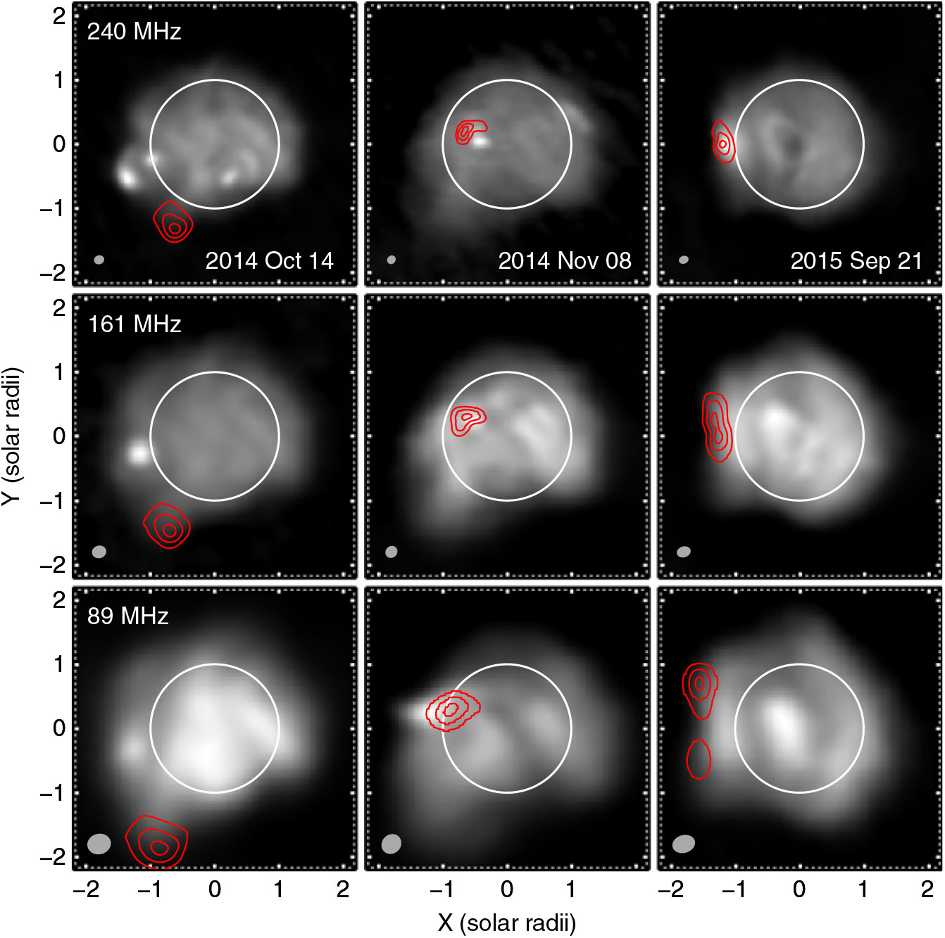
Figure 12. Examples of Phase I solar observations at three frequencies on three different days. The grayscale images reflect the quiescent background over a 5-min period, and the red contours show type III bursts. Contour levels are at 30%, 60%, and 90% of the peak intensity, and the total irradiance during burst periods exceeds the background by at least an order of magnitude. The solid white circle denotes the optical disk, and the gray ellipses represent the synthesised beam sizes. The burst site on 21 September 2015 (right column) elongates and ultimately splits into two components with decreasing frequency due to a diverging magnetic field structure (McCauley et al. Reference McCauley, Cairns, Morgan, Gibson, Harding, Lonsdale and Oberoi2017). Structure can also be seen in the 8 November 2014 burst (middle panel), but it is difficult to interpret given the low-spatial resolution.
Below we summarise the work done with the Phase I MWA and outline how this work will be extended with the Phase II MWA. These efforts are also leading toward the realisation of SKA1-Low and its solar science goals (Nindos et al. Reference Nindos, Kontar and Oberoi2019).
6.1.1. Calibration and imaging challenges
At MWA frequencies, even the quiet Sun is orders of magnitude brighter than any Southern-hemisphere compact source, with radio bursts reaching flux densities many orders of magnitude brighter still. This means that there is sufficient signal to noise to image the Sun easily, even when using a very short snapshot with extremely narrow bandwidth. However, it also means that astrophysical sources are not typically visible when viewing the Sun unless extremely high dynamic range can be attained. Consequently, a technique was developed for robust absolute flux density calibration using a sky model of diffuse Galactic emission (Oberoi et al. Reference Oberoi, Sharma and Rogers2017). This technique exploits the MWA’s wide FOV and numerous short baselines to which the Sun appears as an unresolved source. Only a few baselines are required (and no imaging is necessary) making the technique computationally lean. A prescription to transfer this flux calibration to solar images has also been developed (Mohan & Oberoi Reference Mohan and Oberoi2017).
In order to follow the spatial, spectral, and temporal evolution of solar emission, it is desirable to image the Sun with the maximum time and frequency resolution possible (typically 0.5 s and 40 kHz time and frequency resolution, respectively). However, this can mean $\sim1\!\times10^5$
images per minute of observation. Therefore, in order to be able to analyse significant amounts of MWA data, it is imperative to use automated pipelines for calibration and imaging. This has motivated the development of an Fermi Automated Imaging Routine for Compact Arrays for Radio Sun (AIRCARS; Mondal et al. Reference Mondal, Mohan, Oberoi, Morgan, Benkevitch, Lonsdale, Crowley and Cairns2019b). This end-to-end interferometric calibration and imaging pipeline also corrects for bandwidth decorrelation due to differing cable lengths, tunes the analysis to the needs of solar imaging, and is able to improve imaging quality well beyond what had been achieved by other fully automated approaches. AIRCARS has successfully been used in a completely hands-off manner for imaging data spanning a large range of solar conditions (peak brightness temperatures ranging from
$\sim1\!\times10^5$
images per minute of observation. Therefore, in order to be able to analyse significant amounts of MWA data, it is imperative to use automated pipelines for calibration and imaging. This has motivated the development of an Fermi Automated Imaging Routine for Compact Arrays for Radio Sun (AIRCARS; Mondal et al. Reference Mondal, Mohan, Oberoi, Morgan, Benkevitch, Lonsdale, Crowley and Cairns2019b). This end-to-end interferometric calibration and imaging pipeline also corrects for bandwidth decorrelation due to differing cable lengths, tunes the analysis to the needs of solar imaging, and is able to improve imaging quality well beyond what had been achieved by other fully automated approaches. AIRCARS has successfully been used in a completely hands-off manner for imaging data spanning a large range of solar conditions (peak brightness temperatures ranging from $10^6$
to
$10^6$
to $10^9$
K) and can routinely produce images with dynamic ranges between
$10^9$
K) and can routinely produce images with dynamic ranges between $10^3$
and
$10^3$
and $10^5$
.
$10^5$
.
6.1.2. Radio bursts
Type III bursts are caused by semi-relativistic electron beams that stream through and perturb the background plasma, generating Langmuir waves that ultimately produce intense radio emission. The electrons are accelerated by magnetic reconnection during solar flares, which was directly evidenced by observations from the 32-tile MWA prototype (Cairns et al. Reference Cairns2018), and the beams then propagate away from the Sun along magnetic field lines connected to the flare site. In particular, this analysis showed definitive evidence for reconnection occurring in association with type III bursts and with X-ray emissions. Additionally, since the associations are not 1:1 in either direction, special conditions are required to produce observable radio emissions and X-rays.
McCauley et al. (Reference McCauley, Cairns, Morgan, Gibson, Harding, Lonsdale and Oberoi2017) reported on Phase I MWA observations of type III source regions that repetitively split apart in a direction roughly perpendicular to the inferred electron beam trajectory, and they concluded that this behaviour resulted from a distinctive magnetic field configuration implied by contemporaneous extreme-ultraviolet observations. These results highlight the MWA’s capability to probe electron beam trajectories, and thereby local magnetic field structures, in new and unexpected ways. Type III bursts can also be used to probe the coronal density, which was explored by McCauley et al. (Reference McCauley, Cairns and Morgan2018), who found much larger densities than expected from standard models. This replicated decades-old findings from previous instruments, and MWA observations of the quiescent corona were used to estimate the extent to which the type III source heights were altered by radio propagation effects, which were found to be important but not entirely sufficient to explain the apparent density enhancements. Comparisons between observations of the scattered source (which includes any angular broadening and ducting) and simulations which typically ignore these effects offer one way to determine the impact of these processes. Since some observations (Mercier et al. Reference Mercier, Subramanian, Kerdraon, Pick, Ananthakrishnan and Janardhan2006) and theory suggest that sometimes scattering is very weak and sometimes strong (Subramanian & Cairns Reference Subramanian and Cairns2011), and the amount of scattering depends on a line integral involving the spectrum of density irregularities, these theory-data comparisons might remotely constrain the spectrum and spatial variations of density turbulence in the corona.
Mohan et al. (Reference Mohan, Mondal, Oberoi and Lonsdale2019b) have succeeded in unambiguously disentangling the effects of scattering from intrinsic variations in emission morphology of a weak type III burst. This has led to the discovery of second-scale quasi-periodic oscillations in the angular size and orientation of the burst source with simultaneous oscillations in the intensity of the burst. These observations cannot be explained in terms of the conventional Alfvènic oscillations. In the same data set, Mohan et al. (Reference Mohan, McCauley, Oberoi and Mastrano2019a) also find an unrelated weak flare seen in the EUV and soft X-rays. Their analysis shows that this flare was responsible for some local coronal heating. A detailed study of the radio emissions associated with the magnetic loop undergoing heating has revealed a strong tendency for the observed short-lived narrow-band nonthermal radio emissions to cluster on a timescale of 30 s. This clustering is very well formed and prominent when the heating event is in progress, but is seen to exist even prior to the start of the heating phase, suggesting that this timescale is independent of the heating event itself. This discovery was made possible by the high dynamic range spectroscopic snapshot imaging capability of the MWA, which enabled a reliable detection of the weak nonthermal emissions originating from the source of interest, even in the presence of other stronger activity. The improved PSF of the MWA Phase II and its higher angular resolution will enable detection of even finer features and further increase the imaging dynamic range of MWA solar images.
Type II bursts are interpreted in terms of shocks accelerating electrons that generate Langmuir waves and then radiation at the electron plasma frequency and its harmonic (Nelson & Melrose Reference Nelson and Melrose1985; Cairns Reference Cairns2011). Observational analyses and simulations predict that sometimes multiple regions of the shock produce the radio emission simultaneously or sequentially, depending on the event (Schmidt & Cairns Reference Schmidt and Cairns2012; Schmidt et al. Reference Schmidt, Cairns and Lobzin2014; Kozarev et al. Reference Kozarev, Raymond, Lobzin and Hammer2015). MWA Phase I observations of the 7 September 2014 type II burst show a stably located, weakly/un-resolved source despite predictions for multiple type II subsources a factor of $\sim 4 - 10$
smaller than the beam size at 140 MHz. The increased resolution of MWA Phase II will provide a stronger test of the multiple-source hypothesis.
$\sim 4 - 10$
smaller than the beam size at 140 MHz. The increased resolution of MWA Phase II will provide a stronger test of the multiple-source hypothesis.
Another window on these processes is provided by polarimetry. Studies of the polarised time- and spatially varying source regions of type II and III bursts will also produce new science and constraints on emission mechanisms and scattering processes.
One long-standing issue is that the standard theory for type I, II, and III bursts involves generation of radiation near the electron plasma frequency, that is, 100% circularly polarised in the sense of the ‘ordinary’ (or ‘o’) mode, yet this is not observed for all three: specifically, type Is are almost invariably 100% circularly polarised, type IIs (except for herringbone fine structures) less than $\sim\!20\%$
, and type IIIs are occasionally up to 60% but typically
$\sim\!20\%$
, and type IIIs are occasionally up to 60% but typically $\mathop < \limits_ \sim 20\%$
(Nelson & Melrose Reference Nelson and Melrose1985; Suzuki & Dulk Reference Suzuki and Dulk1985). One interpretation is that the standard theories are wrong but another is that scattering depolarises the radiation (Melrose Reference Melrose2006). MWA Phase II can address these issues by explicitly measuring the time- and spatially varying sources in all four Stokes parameters, searching for evidence of strongly polarised substructures that vary with time and space (e.g. depolarisation fronts moving away from the cores of subsources versus random flickering polarisation regions).
$\mathop < \limits_ \sim 20\%$
(Nelson & Melrose Reference Nelson and Melrose1985; Suzuki & Dulk Reference Suzuki and Dulk1985). One interpretation is that the standard theories are wrong but another is that scattering depolarises the radiation (Melrose Reference Melrose2006). MWA Phase II can address these issues by explicitly measuring the time- and spatially varying sources in all four Stokes parameters, searching for evidence of strongly polarised substructures that vary with time and space (e.g. depolarisation fronts moving away from the cores of subsources versus random flickering polarisation regions).
In conclusion, studies of solar radio bursts are expected to benefit substantially from MWA-Phase II’s improvements in linear spatial resolution (a factor close to 2) and better Fermi uv plane coverage (better imaging fidelity). These should result in much better characterisation of the complex, sub-structured sources of type II and III bursts in position, time, and polarisation, thereby enabling more quantitative tests of theoretical ideas and predictions.
6.1.3. Radio counterparts of coronal mass ejections
The bulk of solar dynamics is dictated by solar magnetic fields, but beyond the photosphere their measurements have remained difficult. Radio observations form the only known techniques to measure these fields. The first successful attempt to model the spectrum of radio emission from the Coronal Mass Ejection (CME) plasma as gyrosynchrotron emission and hence provide an estimate of the CME magnetic field was by Bastian et al. (Reference Bastian, Pick, Kerdraon, Maia and Vourlidas2001). In spite of their well-recognised merits, and considerable effort expended towards them, there are only a handful of successful detections available in the literature (Maia et al. Reference Maia, Gama, Mercier, Pick, Kerdraon and Karlicky2007; Tun & Vourlidas Reference Tun and Vourlidas2013; Bain et al. Reference Bain, Krucker, Saint-Hilaire and Raftery2014; Carley et al. Reference Carley, Vilmer, Simões and Ó Fearraigh2017), some of which are different attempts to model the same CME. The key reason for this lack of success is that the intrinsic $T_B$
of gyrosynchrotron emission is at least a few orders of magnitude lower than that of the other nonthermal emissions usually present during the times when a CME has recently lifted off, and the imaging dynamic range provided by instrumentation available until recently fell short of the requirement to be able to image this weak emission. Recent work with the MWA has shown that with its improved imaging dynamic range, and ability to simultaneously sample its entire observing band, it should now be possible to routinely image the radio counterparts of CMEs and model their spectra in a more robust manner than possible before (Mondal et al. Reference Mondal, Oberoi and Vourlidas2019a). The improved resolution of the MWA Phase II will reveal the structures in CMEs in greater detail and its better imaging dynamic range will permit tracking of these emissions further out into the heliosphere, making these measurements relevant from a space weather perspective.
$T_B$
of gyrosynchrotron emission is at least a few orders of magnitude lower than that of the other nonthermal emissions usually present during the times when a CME has recently lifted off, and the imaging dynamic range provided by instrumentation available until recently fell short of the requirement to be able to image this weak emission. Recent work with the MWA has shown that with its improved imaging dynamic range, and ability to simultaneously sample its entire observing band, it should now be possible to routinely image the radio counterparts of CMEs and model their spectra in a more robust manner than possible before (Mondal et al. Reference Mondal, Oberoi and Vourlidas2019a). The improved resolution of the MWA Phase II will reveal the structures in CMEs in greater detail and its better imaging dynamic range will permit tracking of these emissions further out into the heliosphere, making these measurements relevant from a space weather perspective.
6.1.4. Weak non-thermal emission
Early observations with the 32-element MWA prototype revealed a previously unappreciated abundance of weak, short-lived (few s), narrow-band (few MHz) impulsive nonthermal emission features carpeting the frequency–time plane (Oberoi et al. Reference Oberoi2011). Detailed non-imaging investigations of weak impulsive nonthermal emissions have been carried out using the MWA Phase I with the aim of providing robust statistics on these emissions. Using an automated continuous wavelet transforms-based approach, Suresh et al. (Reference Suresh2017) found that these impulsive emissions take place at the rate of many thousand per hour (as measured across 30.72 MHz bandwidth). Individual emission features were found to last for 1–2 s and span 4–5 MHz in bandwidth and $\sim\! 1-100$
SFU
Footnote e
in peak flux densities. Their characteristics suggest that these features might represent the weaker end of the distribution of solar type I bursts. Using a Gaussian mixtures-based statistical analysis technique, Sharma et al. (Reference Sharma, Oberoi and Arjunwadkar2018) modelled the solar radio emission as a superposition of a slowly varying emission component of thermal origin and an impulsive, and hence nonthermal, component. They estimated the flux density distribution as well as the prevalence of impulsive nonthermal emission in the frequency–time plane. They found the fractional occupancy of nonthermal impulsive emission to lie in the range 17%–45% even during a period of medium solar activity, and that the flux density radiated in the impulsive component is very similar in strength to that radiated in the thermal emission-dominated slowly varying component.
$\sim\! 1-100$
SFU
Footnote e
in peak flux densities. Their characteristics suggest that these features might represent the weaker end of the distribution of solar type I bursts. Using a Gaussian mixtures-based statistical analysis technique, Sharma et al. (Reference Sharma, Oberoi and Arjunwadkar2018) modelled the solar radio emission as a superposition of a slowly varying emission component of thermal origin and an impulsive, and hence nonthermal, component. They estimated the flux density distribution as well as the prevalence of impulsive nonthermal emission in the frequency–time plane. They found the fractional occupancy of nonthermal impulsive emission to lie in the range 17%–45% even during a period of medium solar activity, and that the flux density radiated in the impulsive component is very similar in strength to that radiated in the thermal emission-dominated slowly varying component.
These studies were motivated by the desire to explore the use of weak nonthermal emissions in looking for signatures of weak magnetic reconnection events, the presence of which was originally suggested by Parker (Reference Parker1988). Referred to as the nanoflare hypothesis, the simultaneous presence of a large number of weak reconnection events carpeting the solar surface, but too weak to be detected individually, was proposed as a possible resolution of the coronal heating problem and remains one of the likely possibilities. At flux densities of $\sim 0.2$
SFU, these are the weakest nonthermal emissions reported at low radio frequencies using non-imaging techniques. Ongoing imaging studies using MWA Phase I suggest RMS variability during quiet Sun conditions at the levels of
$\sim 0.2$
SFU, these are the weakest nonthermal emissions reported at low radio frequencies using non-imaging techniques. Ongoing imaging studies using MWA Phase I suggest RMS variability during quiet Sun conditions at the levels of $10^{-3}$
SFU (i.e. 10 Jy), by far the weakest to be reported ever. The high dynamic range techniques described in Sec. 6.1.1 along with the higher angular resolution of MWA Phase II will enable even deeper studies to come. Although a lot remains to be done before their role in coronal heating can be elucidated, these studies have firmly established the presence and abundance of nonthermal emissions significantly weaker than were known before.
$10^{-3}$
SFU (i.e. 10 Jy), by far the weakest to be reported ever. The high dynamic range techniques described in Sec. 6.1.1 along with the higher angular resolution of MWA Phase II will enable even deeper studies to come. Although a lot remains to be done before their role in coronal heating can be elucidated, these studies have firmly established the presence and abundance of nonthermal emissions significantly weaker than were known before.
6.1.5. Quiescent sun
It is not only bursts that are of interest but also sources on the quiescent Sun, for instance, associated with coronal holes, active regions, and the quiet Sun itself. Work with MWA Phase I intensity data shows new features of coronal holes and active regions (McCauley et al. Reference McCauley, Cairns, Morgan, Gibson, Harding, Lonsdale and Oberoi2017). MWA Phase II’s better angular resolution and imaging fidelity will allow better characterisation of these sources and better comparisons with the SDO, SOHO, and RHESSI data from the UV to X-rays.
In addition, recent work using Phase I data has produced the first low-frequency images of the quiescent solar corona in circular polarisation (McCauley et al. Reference McCauley, Cairns, White, Mondal, Lenc, Morgan and Oberoi2019). The Stokes Fermi V structure at the lowest MWA frequencies is found to be generally well-correlated with the structure of the line-of-sight magnetic field component in a widely used global magnetic field model at a height roughly corresponding to that of the radio limb. Coronal magnetic field models are typically extrapolated from photospheric observations, and there are very few observations that can be used to constrain the field at the heights and scales probed by MWA observations. This is a powerful and unique capability of the MWA that will be greatly enhanced by the improved spatial resolution of the Phase II extended mode, as Phase I could not resolve many of the features that would discriminate between competing models.
6.2. Observations of the heliosphere
6.2.1. Interplanetary scintillation
Interplanetary Scintillation (IPS) is the rapid ( $\sim$
1 s) variability in brightness of compact (
$\sim$
1 s) variability in brightness of compact ( $\mathop < \limits_ \sim $
1 arcsecond) sources due to scattering of the propagating wave by the solar wind: a supersonic outflow of turbulent plasma which fills interplanetary space. A detection of IPS with the MWA was first made serendipitously in night-time astrophysical data by Kaplan et al. (Reference Kaplan2015a). Following this, a pilot study was made using observations designed for the purpose, at solar elongations most suitable for detecting IPS (Morgan et al. Reference Morgan2018). This pilot study demonstrated that the MWA has a unique capability for detecting IPS of several hundred sources simultaneously in a single 5-min observation. From a solar science perspective, this means that the heliosphere can be mapped in unprecedented detail in a very short amount of time.
$\mathop < \limits_ \sim $
1 arcsecond) sources due to scattering of the propagating wave by the solar wind: a supersonic outflow of turbulent plasma which fills interplanetary space. A detection of IPS with the MWA was first made serendipitously in night-time astrophysical data by Kaplan et al. (Reference Kaplan2015a). Following this, a pilot study was made using observations designed for the purpose, at solar elongations most suitable for detecting IPS (Morgan et al. Reference Morgan2018). This pilot study demonstrated that the MWA has a unique capability for detecting IPS of several hundred sources simultaneously in a single 5-min observation. From a solar science perspective, this means that the heliosphere can be mapped in unprecedented detail in a very short amount of time.
These findings motivated a 6-month long-observing campaign, described in detail by Morgan et al. (Reference Morgan, Macquart, Chhetri, Ekers, Tingay and Sadler2019). The analysis of these data is ongoing; however, much of the work so far has focused on determining the astrophysical nature of the sources detected. They differ somewhat from compact source populations at higher frequencies, most notably they are dominated by peaked-spectrum sources (Chhetri et al. Reference Chhetri, Morgan, Ekers, Macquart, Sadler, Giroletti, Callingham and Tingay2018a). The precise counts of the various sub-populations are described in Chhetri et al. (Reference Chhetri, Ekers, Morgan, Macquart and Franzen2018b). Sadler et al. (Reference Sadler, Chhetri, Morgan, Mahony, Jarrett and Tingay2019) have shown that the most compact IPS sources are high-redshift sources, 1/3 of which have a redshift $>\!2$
.
$>\!2$
.
A further key finding (Morgan et al. Reference Morgan2018) was the necessity to maximise the sensitivity and imaging fidelity on short timescales ( $\sim$
1 s). In contrast to most astrophysical applications, where MWA sensitivity is limited by confusion noise (see, e.g., Wayth et al. Reference Wayth2015), IPS sources are more rare and therefore the confusion limit is at a considerably lower flux density. However, since IPS detections are made by measuring an increased variance in flux density, the detection limit in an observation only reduces with the fourth root of observing time. This makes maximising the instantaneous sensitivity of the array critical.
$\sim$
1 s). In contrast to most astrophysical applications, where MWA sensitivity is limited by confusion noise (see, e.g., Wayth et al. Reference Wayth2015), IPS sources are more rare and therefore the confusion limit is at a considerably lower flux density. However, since IPS detections are made by measuring an increased variance in flux density, the detection limit in an observation only reduces with the fourth root of observing time. This makes maximising the instantaneous sensitivity of the array critical.
This can be maximised in synthesis images by choosing a natural weighting scheme (where all baselines are weighted equally). However, this comes with two disadvantages: firstly, the resolution is poor compared to a weighting scheme which increases the weight of longer baselines (i.e. a uniform weighting scheme); secondly, the PSF of the array in a naturally weighted image typically has higher sidelobes. With the Phase I MWA, this latter effect is very strong due to the very high concentration of tiles in the core. This is in contrast to uniformly weighted images which have an exceptionally good PSF due to the large number of interferometer elements in the MWA and their pseudo-random arrangement. For IPS observations (where the Sun is typically in the sidelobes), uniform weighting has the added advantage that it downweights the extended quiet Sun significantly.
As shown in Wayth et al. (Reference Wayth2018), by utilising the extended Phase II MWA and using natural weighting, we combine the resolution and exceptionally low sidelobes of uniformly weighted Phase I images with the sensitivity of naturally weighted Phase I images. This should lead to a factor of 2 improvement in sensitivity (Wayth et al. Reference Wayth2015).
6.2.2 Faraday rotation measurements
Kinetic and magnetic energy from a CME can create major, potentially damaging disturbances in the near-earth environment, and there is high interest in being able to predict both the arrival time and the effects of CME impacts with sufficient precision and lead-time. Since the geo-effectiveness of CME impacts is strongly dependent on the orientation of the magnetic field in the CME, a long-standing goal of low-frequency observations in the context of space weather is to measure the orientation of the magnetic fields in propagating CMEs. The only known means of remote detection of this orientation is via the measurement of Faraday rotation (FR) in the plasma of the CME (Oberoi & Lonsdale Reference Oberoi and Lonsdale2012).
Because of the radial dependence of coronal/solar wind density and magnetic field strength, attempts to detect FR from heliospheric plasma, and in particular from CME events, have been confined to regions close to the sun. Some measurements have used linearly polarised signals from spacecraft (e.g. the Helios spacecraft at distances of 2–20 solar radii, using the 2.295 GHz carrier or the MESSENGER spacecraft using the 8 GHz carrier, probing the corona at a few solar radii Hollweg et al. Reference Hollweg, Bird, Volland, Edenhofer, Stelzried and Seidel1982; Jensen et al. Reference Jensen, Nolan, Bisi, Chashei and Vilas2013; Efimov et al. Reference Efimov, Lukanina, Rogashkova, Samoznaev, Chashei, Bird and Paetzold2015). Others have used pulsars (Ord et al. Reference Ord, Johnston and Sarkissian2007; You et al. Reference You, Coles, Hobbs and Manchester2012), again at small solar elongations where the coronal plasma and field strengths are high. Observations of polarised extragalactic sources have also been conducted (e.g. Le Chat et al. Reference Le Chat, Kasper, Cohen and Spangler2014), most recently with considerable success using the upgraded Karl G. Jansky VLA (Kooi et al. Reference Kooi, Fischer, Buffo and Spangler2017), also at small solar elongations. The pulsar and extragalactic source observations have typically been done at low GHz frequencies.
In order to probe heliospheric and CME FR at large fractions of an au, much lower frequencies must be used so that the amount of rotation is detectable. This requires that a source of background linearly polarised emission must be present, but discrete polarised sources tend to be few and weak at MWA frequencies. Furthermore, to be of practical utility, any FR measurements must target the inner heliosphere for CMEs which may be on a collision course, which generally means performing the FR observations during the daytime. Due to the strength of solar radio emission, this places extraordinary demands on the imaging dynamic range of these observations.
The MWA Phase I system has allowed major advances in these studies for two key reasons. First, as has been demonstrated by MWA observations (Lenc et al. Reference Lenc2016), the polarised galactic synchrotron background has much more power on large angular scales than on small scales, a discovery made possible by the excellent short-baseline Fermi uv coverage and imaging capability of the MWA. Thus, by employing low angular resolution imaging, a strong polarised signal against which to measure FR is readily available in essentially all directions. This is a dramatically more favourable scenario than trying to use a sparse grid of weak polarised discrete sources. Second, the excellent instantaneous Fermi uv coverage of the MWA combined with thousands of independent closure quantities has allowed the development of very high dynamic range solar imaging, which in turn creates a realistic possibility of detecting much weaker emission (the polarised Galactic background) during the daytime, and making FR measurements of CME plasma in the inner heliosphere. Work continues to further improve dynamic range via the development of direction-dependent ionospheric calibration on small linear scales.
For FR work, the Phase II system differs from Phase I in one important respect, namely that for either high or low angular resolution work, essentially all 128 tiles are available, instead of a subset. For low-resolution FR studies, the compact configuration thus yields not only greater sensitivity but also denser Fermi uv coverage with extensive redundancy (by design) to constrain calibration solutions. Improved calibration, the inclusion of direction-dependent, small linear scale ionospheric calibration, and the much simpler nature of the angular structure of the solar emission on scales of $0.5^{\circ}$
and larger combine to offer the prospect of meaningful daytime FR measurements. Such measurements are potentially possible using existing Phase I data, but compact configuration Phase II data will be inherently superior.
$0.5^{\circ}$
and larger combine to offer the prospect of meaningful daytime FR measurements. Such measurements are potentially possible using existing Phase I data, but compact configuration Phase II data will be inherently superior.
The first detection and characterisation of spatially resolved FR associated with an interplanetary CME would be a major result, offering a densely sampled large-volume view of a quantity directly related to the magnetic field geometry. This would transform studies of CME dynamics and would point the way to a future network of low-frequency imaging arrays, modelled after the MWA, that could form a crucial part of a space weather prediction network.
6.3. Observations of the ionosphere
During Phase I, ionospheric research has been driven largely by the needs of individual science teams to measure and compensate for the effects of the ionosphere on their own observations (e.g. Loi et al. Reference Loi2015b; Jordan et al. Reference Jordan2017). Additionally, (Arora et al. Reference Arora2015; Arora et al. Reference Arora2016) have investigated the possibility of using GPS measurements to assist in low-frequency radio astronomy calibration.
This work has shown that the refractive shifts of radio sources at MWA frequencies allow measurements of the density gradient of the ionosphere with unprecedented accuracy and (thanks to the sensitivity and wide FOV of the MWA) with an unprecedented number of pierce points. These practically motivated investigations have nonetheless led to unexpected discoveries. Most notably, Loi et al. (Reference Loi2015a) discovered strikingly regular linear features in the observed refractive shifts in radio sources. Through careful investigations, including splitting the array to measure distance via parallax, it was shown that these features are located within the magnetosphere and follow the Earth’s magnetic field lines.
More recently, ongoing work using AIRCARS under a diverse range of solar conditions has led to the conclusion that the variations in the ionospheric phase across the $\sim0.5^{\circ}$
radio Sun are the next most constraining bottleneck limiting the imaging dynamic range (Mondal et al. Reference Mondal, Mohan, Oberoi, Morgan, Benkevitch, Lonsdale, Crowley and Cairns2019b). The large flux density of the Sun is in such a high SNR regime that solar imaging is sensitive to small changes in the relative Total Electron Content (TEC):
$\sim0.5^{\circ}$
radio Sun are the next most constraining bottleneck limiting the imaging dynamic range (Mondal et al. Reference Mondal, Mohan, Oberoi, Morgan, Benkevitch, Lonsdale, Crowley and Cairns2019b). The large flux density of the Sun is in such a high SNR regime that solar imaging is sensitive to small changes in the relative Total Electron Content (TEC): $\sim$
1 mTECU (where
$\sim$
1 mTECU (where $1\,\text{TECU}\,=\,10^{16}\,\text{electrons m}^{-2}$
) over small spatial (
$1\,\text{TECU}\,=\,10^{16}\,\text{electrons m}^{-2}$
) over small spatial ( $\sim$
few 100 m) and temporal (
$\sim$
few 100 m) and temporal ( $\sim$
10 s) scales. In calibrating out these effects, we will directly measure the ionosphere on much smaller scales than previous MWA work, but with the same unprecedented accuracy.
$\sim$
10 s) scales. In calibrating out these effects, we will directly measure the ionosphere on much smaller scales than previous MWA work, but with the same unprecedented accuracy.
7. Other opportunities
While the majority of MWA collaboration efforts fall under the four primary science themes, the instrument’s flexibility offers other opportunities as well. Here, we highlight new directions that have developed since the original conception of the telescope.
7.1. Space situational awareness
The MWA was first used to detect objects in low Earth orbit (LEO) while the array was still being commissioned (Tingay et al. Reference Tingay2013b). This initial investigation used correlated data to image the sky and detect FM radio broadcasts reflected from the International Space Station (ISS) as it transited over Western Australia. In a study designed to detect radio emission from fireballs, Zhang et al. (Reference Zhang2018) serendipitously detected numerous objects in LEO, including the ISS (100 m diameter), the Advanced Land Observing Satellite (10 m), the defunct satellite Alouette-2 (1 m), and the cube-sat Duchifat-1 (10 cm). By mapping the location of LEO objects during their passage through the FOV of the MWA, it is possible to recreate their orbital parameters. With the resolution of the Phase I MWA, objects in LEO can be located to well within the nominal 1 km error ellipse that accompanies the orbital parameters listed in the TLE catalogue. The detection of objects smaller than the ISS validates the predictions of Tingay et al. (Reference Tingay2013b) and demonstrates the capability of using the MWA to both monitor and detect objects in LEO, including space debris, allowing the MWA to contribute to Australian and global Space Situational Awareness (SSA).
The MWA has been used as the receiving station of a passive bi-static radar system to again detect the ISS as well as aircraft and meteors trails (Palmer et al. Reference Palmer2017). In the passive bi-static radar set-up, terrestrial broadcast stations (in the FM range $80-108$
MHz) are used as illuminators of opportunity. The MWA records baseband data using the VCS and forms beams on the expected location of the ISS, and in the direction of the Geraldton or Perth-based stations. This is the set-up used by Palmer et al. (Reference Palmer2017); however, the maximum expected degree of correlation between the direct and reflected signals is less than unity due to the corrupting effects of the ionosphere as it diffracts the direct signal over the horizon and into the FOV of the MWA. Using data captured at sites local to the FM broadcast stations in Perth has been shown to work well and increase the degree of correlation between the direct and reflected signals (Hennessy et al. Reference Hennessy2019). The use of radar techniques to detect and monitor objects in LEO means that the MWA can determine not only the location of the objects but also the line of sight distance, velocity, and acceleration.
$80-108$
MHz) are used as illuminators of opportunity. The MWA records baseband data using the VCS and forms beams on the expected location of the ISS, and in the direction of the Geraldton or Perth-based stations. This is the set-up used by Palmer et al. (Reference Palmer2017); however, the maximum expected degree of correlation between the direct and reflected signals is less than unity due to the corrupting effects of the ionosphere as it diffracts the direct signal over the horizon and into the FOV of the MWA. Using data captured at sites local to the FM broadcast stations in Perth has been shown to work well and increase the degree of correlation between the direct and reflected signals (Hennessy et al. Reference Hennessy2019). The use of radar techniques to detect and monitor objects in LEO means that the MWA can determine not only the location of the objects but also the line of sight distance, velocity, and acceleration.
LEO constitutes orbits of less than $2\,000$
km, whereas the longest baselines of MWA Phase I have a near/far field transition that is at
$2\,000$
km, whereas the longest baselines of MWA Phase I have a near/far field transition that is at $4\,800$
km (at 80 MHz). In the work of Zhang et al. (Reference Zhang2018), only baselines shorter than 387 m were imaged to ensure satellites and meteors were in the far field of the MWA. Because not all Phase I baselines were able to be used, the final sensitivity was reduced. The Phase II compact configuration of the MWA contains many more short baselines than the Phase I configuration and will therefore translate to an increase in sensitivity for observing objects in LEO, and an increased capability for SSA.
$4\,800$
km (at 80 MHz). In the work of Zhang et al. (Reference Zhang2018), only baselines shorter than 387 m were imaged to ensure satellites and meteors were in the far field of the MWA. Because not all Phase I baselines were able to be used, the final sensitivity was reduced. The Phase II compact configuration of the MWA contains many more short baselines than the Phase I configuration and will therefore translate to an increase in sensitivity for observing objects in LEO, and an increased capability for SSA.
7.2. Search for extraterrestrial intelligence
The SETI has been reinvigorated in recent years, in part by the realisation that many stars are orbited by planets with conditions suitable for life as we know it, and also by the launch of major new SETI initiatives such as BL (Worden et al. Reference Worden2017), which is currently undertaking a pilot project at MWA.
The MWA has several characteristics that make it ideal for SETI surveys, including:
A wide FOV, so that a typical pointing contains many targets of interest, and so that much of the sky is covered to a depth of at least several hours each year
Flexible digital back-ends, enabling commensal surveys (beamforming for SETI without the need to control the primary beam pointing) and the generation of high-resolution spectra from low-level raw voltage data
An extremely radio-quiet site, minimising the major contaminant in any SETI survey—human-generated radio frequency interference (RFI)
Access to an under-explored region of the radio spectrum that may be very promising for the detection of bright extraterrestrial transmitters similar to those produced by human civilisation (Loeb & Zaldarriaga Reference Loeb and Zaldarriaga2007).
The MWA has already undertaken SETI experiments (Tingay et al. Reference Tingay, Tremblay, Walsh and Urquhart2016; Tingay et al. Reference Tingay, Tremblay and Croft2018a,b) using data cubes generated by the correlator that were gathered for other primary science goals, and subsequently searched for candidate SETI signals. Similar studies could be done in Phase II (with improved angular resolution), but the new capabilities of the array can provide additional advantages. SETI is one of a handful of science areas that was not covered in the original MWA science paper (Bowman et al. Reference Bowman2013), but has now become a substantial area of research at MWA in part as a result of experience gained during Phase I.
The improved angular resolution in the MWA Phase II’s extended configuration will allow more precise localisation of candidate SETI signals. Higher spectral resolution from the correlator improvements currently underway, along with real-time beamforming planned as part of the BL engagement, will enable better fidelity both for narrow-band signals that have been the target of the majority of previous SETI searches and better classification of more complex and broadband signals. In addition to allowing a more powerful SETI search, these improvements may enable better RFI detection, classification, and rejection.
7.3. Archive analysis
The MWA data archive provides public access to all raw visibility data and a subset of VCS data from both Phase I and Phase II of the instrument. The archive is accessible through the All-Sky Virtual Observatory (ASVO) at http://asvo.mwatelescope.org using a web dashboard or a Python-based API or commandline client. Data are typically made public on the archive 18 months after its initial collection. The archive contains 12 Petabytes (PB) of Phase I data spanning mid-2013 to mid-2016, including 2.5 PB of VCS data. It currently contains 18 PB of Phase II data collected so far since 1 October 2016, of which approximately 70% is from the extended array configuration and 4 PB is VCS data. The AVSO interface has completed approximately 45 000 job requests to date and served over 1.3 PB to users.
Archived Phase II data were recently used by Tingay et al. (Reference Tingay2018b) to perform an after-the-fact search for emitted signals from 1I/2017 U1 ‘Oumuamua to test the speculative possibility that the object is associated with extraterrestrial intelligent life. The study used serendipitous observations identified in the archive by comparing the orbital trajectory of ‘Oumuamua with the target field positions and acquisition times of archived data. An 86-second data set was found that overlapped with the ‘Oumuamua trajectory in 2 months of archived data spanning 2017 November 1 through 2018 January 10, when the search was performed.
Similarly, Croft et al. (Reference Croft2016) used archival MWA data to search for radio transient emission coincident with two candidate high-energy neutrino events detected by the ANTARES neutrino telescope. No counterparts were detected, but they were able to place upper limits on progenitors in host galaxies within the localisation of the neutrino events ( $10 \times 10^{37}\, \text{ergs}^{1}$
at 20 Mpc) and redshift limits if the source was not from the nearby galaxies (
$10 \times 10^{37}\, \text{ergs}^{1}$
at 20 Mpc) and redshift limits if the source was not from the nearby galaxies ( $z\geq0.2$
).
$z\geq0.2$
).
The large FOV of the MWA greatly increases the likelihood that the data archive contains observations of a given part of the sky at any time. The typical MWA field size of $500-1000\,\text{deg}^2$
translates to approximately 2.5%–5% of the southern sky observed at any given time. This makes the MWA archive more effective for follow-up of transient events compared to data archives of dish-based telescopes with smaller fields of view. Furthermore, the archive contains observations of the entire sky below +30 declination, as well as thousands of hours of repeated observations for a subset of the sky covering more than
$500-1000\,\text{deg}^2$
translates to approximately 2.5%–5% of the southern sky observed at any given time. This makes the MWA archive more effective for follow-up of transient events compared to data archives of dish-based telescopes with smaller fields of view. Furthermore, the archive contains observations of the entire sky below +30 declination, as well as thousands of hours of repeated observations for a subset of the sky covering more than $2000\, \text{deg}^2$
that is revisited nightly for months.
$2000\, \text{deg}^2$
that is revisited nightly for months.
8. Conclusion
The capabilities of the MWA afforded by compact and extended array configurations, new digital back-ends, and a rapid-response triggering system offer opportunities for improved and new science programs. We have outlined here many ways in which the four original science themes of the MWA collaboration will continue to explore the low-frequency astrophysical sky with the Phase II upgrade. In addition, we outlined new directions outside the original themes. As an SKA low-band precursor, the MWA has and continues to be a rich test bed for science and technical demonstrations.
The Phase II upgrade has added to the MWA’s strength as a flexible multi-purpose instrument. The extended configuration has greatly enhanced the potential for high-resolution galaxy surveys and foreground modelling for the EoR studies, while the compact configuration yields very high sensitivity to diffuse emission and a unique hybrid layout to test analysis techniques. The new rapid-response triggering system makes the MWA an excellent instrument for follow-up observations of transient events triggered from EM and multi-messenger signals.
With the MWA’s versatile design, flexible observing modes, Open Skies policy, and public data access through the All-Sky Virtual Observatory, it will continue to serve the astronomical community and produce fruitful scientific results for years to come.
Acknowledgements
The MWA Phase II upgrade project was supported by Australian Research Council LIEF grant LE160100031 and the Dunlap Institute for Astronomy and Astrophysics at the University of Toronto. Parts of this research were supported by the Australian Research Council Centre of Excellence for All Sky Astrophysics in 3 Dimensions (ASTRO 3D), through project number CE170100013. APB is supported by an NSF Astronomy and Astrophysics Postdoctoral Fellowship under award AST-1701440. CMT is supported by an ARC Future Fellowship under grant FT180100321. GEA is the recipient of an Australian Research Council Discovery Early Career Researcher Award (project number DE180100346). SC and the pilot Breakthrough Listen SETI program are supported through the Breakthrough Initiatives, sponsored by the Breakthrough Prize Foundation. D.K. was additionally supported by NSF grant AST-1816492. GG acknowledges the postdoctoral research fellowship by CSIRO. SWD acknowledges an Australian Government Research Training Programme scholarship administered through Curtin University.
This scientific work makes use of the Murchison Radio-astronomy Observatory, operated by CSIRO. We acknowledge the Wajarri Yamatji people as the traditional owners of the Observatory site. Support for the operation of the MWA is provided by the Australian Government (NCRIS), under a contract to Curtin University administered by Astronomy Australia Limited. We acknowledge the Pawsey Supercomputing Centre which is supported by the Western Australian and Australian Governments.