


1. Introduction
The Australian SKA Pathfinder (ASKAP; Hotan et al. Reference Hotan2021), located at Inyarrimanha Ilgari Bundara, the CSIROFootnote 1 Murchison Radio-astronomy Observatory in Western Australia, is a survey radio telescope that operates with a 288-MHz bandwidth between 700 and 1 800 MHz. ASKAP features a unique Phased Array Feed (PAF; Hotan et al. Reference Hotan2014; McConnell et al. Reference McConnell2016) which allows the formation of 36 primary beams covering up to $\sim$
31 deg
$\sim$
31 deg $^{2}$
. This instantaneous wide field of view coupled with
$^{2}$
. This instantaneous wide field of view coupled with $36\times12$
m antennas—with baselines ranging from 22 to 6 km—provides the basis for an instrument optimised for survey speed, with the capability to rapidly survey
$36\times12$
m antennas—with baselines ranging from 22 to 6 km—provides the basis for an instrument optimised for survey speed, with the capability to rapidly survey $\sim$
80% of the sky to heretofore unseen sensitivity.
$\sim$
80% of the sky to heretofore unseen sensitivity.
The Rapid ASKAP Continuum Survey (RACS) is a multi-wavelength survey covering the sky up to $\delta_{\text{J2000}} \lesssim +50^{\circ}$
(McConnell et al. Reference McConnell2020, hereinafter, Reference McConnellPaper I). The survey is being conducted within the three operating bands used by ASKAP. For RACS, these three bands are centred on effective frequencies of 887.5, 1 367.5, and 1 632.5 MHz. As the name suggests, RACS is a shallow survey with 15-min total integration per pointing reaching median root-mean-square (rms) noise between
$\delta_{\text{J2000}} \lesssim +50^{\circ}$
(McConnell et al. Reference McConnell2020, hereinafter, Reference McConnellPaper I). The survey is being conducted within the three operating bands used by ASKAP. For RACS, these three bands are centred on effective frequencies of 887.5, 1 367.5, and 1 632.5 MHz. As the name suggests, RACS is a shallow survey with 15-min total integration per pointing reaching median root-mean-square (rms) noise between $\sim$
200–260
$\sim$
200–260 $\mu$
Jy PSF
$\mu$
Jy PSF $^{-1}$
across the three bands. Due to its baseline distribution, ASKAP has excellent snapshot (u,v) coverage, providing a well-constrained point spread function (PSF) at zenith (
$^{-1}$
across the three bands. Due to its baseline distribution, ASKAP has excellent snapshot (u,v) coverage, providing a well-constrained point spread function (PSF) at zenith ( $\delta_{\text{J2000}} \approx -27^{\circ}$
) with elongation of the major axis for lower-elevation pointings. The resultant median angular resolution of the whole survey across the three bands is in the range
$\delta_{\text{J2000}} \approx -27^{\circ}$
) with elongation of the major axis for lower-elevation pointings. The resultant median angular resolution of the whole survey across the three bands is in the range $\sim$
9–18 arcsec. The goal of RACS is to provide a global sky model for calibration and validation of other ASKAP observations, and once images and source catalogues are available work can be done matching and spectrally modelling sources across the three bands.
$\sim$
9–18 arcsec. The goal of RACS is to provide a global sky model for calibration and validation of other ASKAP observations, and once images and source catalogues are available work can be done matching and spectrally modelling sources across the three bands.
The first pass of the sky in the lowest frequency band at 887.5 MHz (RACS-low) was released in 2020 and is described in Reference McConnellPaper I. RACS-low features a median rms noise of $\sim$
260
$\sim$
260 $\mu$
Jy PSF
$\mu$
Jy PSF $^{-1}$
and median angular resolution of 18 arcsec. Following the initial data release, a radio source catalogue was constructed and described by Hale et al. (Reference Hale2021, hereinafter Reference HalePaper II). This radio source catalogue contains
$^{-1}$
and median angular resolution of 18 arcsec. Following the initial data release, a radio source catalogue was constructed and described by Hale et al. (Reference Hale2021, hereinafter Reference HalePaper II). This radio source catalogue contains $\sim$ $2.1$
million sources, excluding Galactic latitudes of
$2.1$
million sources, excluding Galactic latitudes of $|b| < 5^{\circ}$
. The catalogue was constructed after combining neighbouring images from the original data release to provide a more uniform sensitivity across the region covering
$|b| < 5^{\circ}$
. The catalogue was constructed after combining neighbouring images from the original data release to provide a more uniform sensitivity across the region covering $-80^{\circ} \leq \delta_{\text{J2000}} \leq +30^{\circ}$
. This catalogue is the first large-area catalogue produced as part of RACS. Alongside the Stokes I total intensity data releases, RACS-low data products are also being used to investigate the polarised sky. Using circular polarisation data products from RACS-low, Pritchard et al. (Reference Pritchard2021) identified radio emission coincident with 33 stars, including 23 new radio star associations in this sample. In linear polarisation, RACS data products are being used to generate Spectra and Polarisation In Cutouts of Extragalactic Sources (SPICE-RACS; Thomson et al. Reference Thomson2023, Reference ThomsonPaper III). The first data release from SPICE-RACS covers a 1 300 deg
$-80^{\circ} \leq \delta_{\text{J2000}} \leq +30^{\circ}$
. This catalogue is the first large-area catalogue produced as part of RACS. Alongside the Stokes I total intensity data releases, RACS-low data products are also being used to investigate the polarised sky. Using circular polarisation data products from RACS-low, Pritchard et al. (Reference Pritchard2021) identified radio emission coincident with 33 stars, including 23 new radio star associations in this sample. In linear polarisation, RACS data products are being used to generate Spectra and Polarisation In Cutouts of Extragalactic Sources (SPICE-RACS; Thomson et al. Reference Thomson2023, Reference ThomsonPaper III). The first data release from SPICE-RACS covers a 1 300 deg $^2$
pilot region and features 5 818 sources with Faraday rotation measures.
$^2$
pilot region and features 5 818 sources with Faraday rotation measures.
The second observing epoch of the sky at 1 367.5 MHz (RACS-mid) was completed in 2021, with follow-up observations taken over 2021–2022, and the first data release is described by Duchesne et al. (Reference Duchesne2023, hereinafter Reference DuchesnePaper IV). RACS-mid data products, along with all available RACS data, are publicly available through the CSIRO ASKAP Science Data Archive (CASDA; Chapman et al. Reference Chapman, Dempsey, Miller, Heywood, Pritchard, Sangster, Whiting, Dart, Lorente, Shortridge and Wayth2017; Huynh et al. Reference Huynh, Dempsey, Whiting, Ophel, Ballester, Ibsen, Solar and Shortridge2020). RACS-mid features a number of changes from RACS-low that helped to improve the overall quality of the survey. These changes include fully autonomous scheduling with a limit to the hour angle of $\pm 1^{\text{h}}$
, peeling and subtraction of bright off-axis sources, bespoke primary beam modelling, and correction of both on-axis and off-axis leakage of Stokes I into V. While RACS-mid has an effective bandwidth of 144-MHz due to radio-frequency interference, the survey still boasts a median rms noise of
$\pm 1^{\text{h}}$
, peeling and subtraction of bright off-axis sources, bespoke primary beam modelling, and correction of both on-axis and off-axis leakage of Stokes I into V. While RACS-mid has an effective bandwidth of 144-MHz due to radio-frequency interference, the survey still boasts a median rms noise of $\sim$
200
$\sim$
200 $\mu$
Jy PSF
$\mu$
Jy PSF $^{-1}$
, which varies smoothly across the sky as a function of declination, except around bright sources. Similarly, because of the close-to-meridian scheduling the angular resolution varies smoothly as a function of declination ranging from 8.1 arcsec near zenith and 47.5 arcsec in the lowest-elevation pointings at high declination. The first RACS-mid data release also included leakage-corrected Stokes V continuum images alongside the Stokes I images for each individual observation.
$^{-1}$
, which varies smoothly across the sky as a function of declination, except around bright sources. Similarly, because of the close-to-meridian scheduling the angular resolution varies smoothly as a function of declination ranging from 8.1 arcsec near zenith and 47.5 arcsec in the lowest-elevation pointings at high declination. The first RACS-mid data release also included leakage-corrected Stokes V continuum images alongside the Stokes I images for each individual observation.
RACS-mid is both competitive with and complementary to existing completed large-area 1.4-GHz radio surveys in the Northern sky such as the NRAOFootnote 2 VLAFootnote 3 Sky Survey (NVSS; Condon et al. Reference Condon, Cotton, Greisen, Yin, Perley, Taylor and Broderick1998) and the Faint Images of the Radio Sky at Twenty Centimeters (FIRST; Becker, White, & Helfand Reference Becker, White and Helfand1995; White et al. Reference White, Becker, Helfand and Gregg1997; Helfand, White, & Becker Reference Helfand, White and Becker2015). In the highest declination strip covered by RACS-mid ( $\delta_{\text{J2000}} = +46^{\circ}$
), the resolution and sensitivity approaches that of the NVSS. For the remainder of the survey the resolution and sensitivity can be expressed as an average of the survey properties of the NVSS and FIRST, with a median angular resolution of
$\delta_{\text{J2000}} = +46^{\circ}$
), the resolution and sensitivity approaches that of the NVSS. For the remainder of the survey the resolution and sensitivity can be expressed as an average of the survey properties of the NVSS and FIRST, with a median angular resolution of $10.1$
arcsec and moderate sensitivity to extended sources up to a few arcmin. RACS-mid data products have so far been used to identify circularly polarised emission from 52 stars that had not previously been detected at radio frequencies (Driessen et al. in preparation), including the detection of circularly polarised emission from a T8 brown dwarf (Rose et al. Reference Rose2023), and have been used in conjunction with FIRST and the VLA Sky Survey (VLASS; Gordon et al. Reference Gordon2021) in a search for radio stars via proper motion (Driessen et al. Reference Driessen, Heald, Duchesne, Murphy, Lenc, Leung and Moss2023). RACS-low and RACS-mid images are also used as an extra epoch for the Variability and Slow Transients (VAST) survey being performed by ASKAP (Murphy et al. Reference Murphy2013, Reference Murphy2021).
$10.1$
arcsec and moderate sensitivity to extended sources up to a few arcmin. RACS-mid data products have so far been used to identify circularly polarised emission from 52 stars that had not previously been detected at radio frequencies (Driessen et al. in preparation), including the detection of circularly polarised emission from a T8 brown dwarf (Rose et al. Reference Rose2023), and have been used in conjunction with FIRST and the VLA Sky Survey (VLASS; Gordon et al. Reference Gordon2021) in a search for radio stars via proper motion (Driessen et al. Reference Driessen, Heald, Duchesne, Murphy, Lenc, Leung and Moss2023). RACS-low and RACS-mid images are also used as an extra epoch for the Variability and Slow Transients (VAST) survey being performed by ASKAP (Murphy et al. Reference Murphy2013, Reference Murphy2021).
At 1 367.5 MHz, ASKAP is also undertaking the Widefield ASKAP L-band Legacy All-sky Blind surveY (WALLABY), which is a neutral hydrogen survey being performed over the next five years with using the same frequency band as RACS-mid (Koribalski et al. Reference Koribalski2020). While WALLABY is primarily a spectral line survey, the 10-h observations and subsequent imaging also result in deep 1 367.5-MHz continuum images. Currently pre-pilot observations of the Eridanus supergroup (For et al. Reference For2021) have been utilised to create an initial WALLABY continuum catalogue (hereinafter the WALLABY prepilot catalogue; Grundy et al. Reference Grundy2023) containing 9 416 sources covering $\sim$
42 deg
$\sim$
42 deg $^{2}$
.
$^{2}$
.
In this fifth paper in the RACS series, we describe the cataloguing of the RACS-mid Stokes I data. Although Stokes V continuum images are available, cataloguing circularly polarised sources with RACS-mid will be described in a future work.
2. Catalogue creation
In cataloguing the RACS-mid Stokes I data, we follow the steps outlined for the construction of the RACS-low catalogue described by Reference HalePaper II. We make some changes to this process to better suit the current data products. As a departure from Reference HalePaper II, we opted to create a primary catalogue for general purpose use, as well as two auxiliary catalogues for more specific uses. The three catalogues cover the normal uses for Stokes I source catalogues, each with their own limitations and strengths. In the following sections, we describe the general steps taken to construct the catalogues, including selection of which observations to include (Section 2.1), making full-sensitivity images (Section 2.2), source-finding (Section 2.3), and merging source lists and duplicate removal (Section 2.4). The primary catalogue and the two auxiliary catalogues are described in Section 3 and are created following the relevant subset of the following steps.
2.1. Image selection
As part of the RACS-mid observing process, some fields were observed and imaged several times. Fields have the naming convention RACS_HHMM $\pm$
DD, and most duplicate field observations and their resultant Stokes I and V images are made available through CASDA. As described in Section 2.1 in Reference DuchesnePaper IV, some of these re-observations were intended to provide a higher-resolution or to account for observations of
$\pm$
DD, and most duplicate field observations and their resultant Stokes I and V images are made available through CASDA. As described in Section 2.1 in Reference DuchesnePaper IV, some of these re-observations were intended to provide a higher-resolution or to account for observations of $<$
12 min (see Section 2.1 in Reference DuchesnePaper IV). Fields that were re-observed due to fatal errors with the instrument are not considered. We define a ‘good’ subset of observed fields to use in the cataloguing process. Each RACS-mid observation has a dedicated scheduling block ID (SBID) which is used as a unique identifier. The selection of which SBID to use when multiple observations exist for a given field is based on the following criteria:
$<$
12 min (see Section 2.1 in Reference DuchesnePaper IV). Fields that were re-observed due to fatal errors with the instrument are not considered. We define a ‘good’ subset of observed fields to use in the cataloguing process. Each RACS-mid observation has a dedicated scheduling block ID (SBID) which is used as a unique identifier. The selection of which SBID to use when multiple observations exist for a given field is based on the following criteria:
-
1. If either duplicate SBID had bright sources peeled (as described in Section 2.3.3 of Reference DuchesnePaper IV), then use the SBID that has undergone peeling,
-
2. Else if either duplicate SBIDs have $<$
12 m total integration time, then Use the SBID with the longest integration time,
$<$
12 m total integration time, then Use the SBID with the longest integration time, -
3. Else if the difference in PSF major axes is
$>$
$2^{\prime\prime}$
between duplicate SBIDs, then select the SBID with the smaller PSF major axes, -
4. Else select the SBID with the lowest median rms noise.


The ordering is important, as peeling in a small number of cases was required to remove CLEAN divergence artefacts but was not necessarily done on the highest-resolution image. The SBIDs with $<$
12 m total integration time are significantly less sensitive than their re-observations so naturally should not be used when more sensitive observations exists. No short observations had better PSF or noise properties than their respective re-observations, and none of these short observations underwent peeling. Finally, resolution and noise properties are often closely related due to their direct relationship to (u,v) coverage, and we find that generally the selection is based on the PSF size rather than the median rms noise if criteria (1) and (2) are not met. A single field was observed three times (RACS_1844+46), though only in the second observation was 3C 380 peeled and is chosen as the good SBID. The selection of good SBIDs is noted in the RACS database fileFootnote 4 under the column SELECT, where SELECT=1 indicates the SBID is selected as part of the good SBID subset. We note that SBIDs not part of this subset can still be used for other science cases and may be particularly useful for variability or transient source studies. The selection is based on the Stokes I images only, and future work with Stokes V may wish to select different SBIDs if noise properties vary between them.
$<$
12 m total integration time are significantly less sensitive than their re-observations so naturally should not be used when more sensitive observations exists. No short observations had better PSF or noise properties than their respective re-observations, and none of these short observations underwent peeling. Finally, resolution and noise properties are often closely related due to their direct relationship to (u,v) coverage, and we find that generally the selection is based on the PSF size rather than the median rms noise if criteria (1) and (2) are not met. A single field was observed three times (RACS_1844+46), though only in the second observation was 3C 380 peeled and is chosen as the good SBID. The selection of good SBIDs is noted in the RACS database fileFootnote 4 under the column SELECT, where SELECT=1 indicates the SBID is selected as part of the good SBID subset. We note that SBIDs not part of this subset can still be used for other science cases and may be particularly useful for variability or transient source studies. The selection is based on the Stokes I images only, and future work with Stokes V may wish to select different SBIDs if noise properties vary between them.
2.2. Full-sensitivity images
A 12% cut-off in the primary beam attenuation was used for primary beam correction and weighting the PAF beam mosaics for each observation. One of the unfortunate features of the linear mosaicking of individual PAF beam images is a tile mosaic with non-rectangular image boundaries and the usual primary beam roll-off. This results in an irregular tile image border that follows the 12% contour of the outer beams. From a science standpoint, the primary beam roll-off limits detection of sources towards image boundaries due to a drop in sensitivity. From a user-perspective, rectangular images with large, irregular areas of blanked pixels can make identifying which sources lie in which image difficult.
As RACS is observed with an overlap between adjacent observations that is at least the PAF beam separation (0.9 degrees for RACS-mid), we follow Reference HalePaper II and use SWarp (Bertin et al. Reference Bertin, Mellier, Radovich, Missonnier, Didelon, Morin, Bohlender, Durand and Handley2002) to form a linear mosaic of adjacent tiles to create rectangular images with full sensitivity towards the image edges. We use the same weight maps used during PAF beam linear mosaicking to ensure the sensitivity profile is consistent across the full image. All adjacent tiles within a group are convolved to a common resolutionFootnote 5 prior to mosaicking. We create one set of images convolved to the lowest common resolution of neighbouring images, and a second set convolved to a fixed 25-arcsec resolution. These images are provided as part of this data release. Convolving to the lowest common resolution results in mosaics that are close to the full resolution of the survey. These full-sensitivity images are created for Stokes I and V, though only Stokes I images are part of this data release. For the 25-arcsec images, we also increase the pixel size by a factor two in each celestial coordinate (i.e. from $2^{\prime\prime} \times 2^{\prime\prime}$
to
$2^{\prime\prime} \times 2^{\prime\prime}$
to $4^{\prime\prime} \times 4^{\prime\prime}$
) to reduce the image file size. The 25-arcsec full-sensitivity images (and catalogue) are restricted to
$4^{\prime\prime} \times 4^{\prime\prime}$
) to reduce the image file size. The 25-arcsec full-sensitivity images (and catalogue) are restricted to $\delta_{\text{J2000}} \lesssim +30^{\circ}$
, similar to RACS-low, as the PSF major axis for some of the original images becomes larger than 25 arcsec beyond this declination.
$\delta_{\text{J2000}} \lesssim +30^{\circ}$
, similar to RACS-low, as the PSF major axis for some of the original images becomes larger than 25 arcsec beyond this declination.
Fig. 1 shows example sources as they appear in the full-sensitivity images compared to the 25-arcsec image from RACS-low (Reference HalePaper II), and comparison optical data from from the Dark Energy Survey data release 2 (DES DR2; Flaugher et al. Reference Flaugher2015; Abbott et al. Reference Abbott2018, Reference Abbott2021). Fig. 1(i) shows an example of radio sources projected onto the galaxy cluster Abell 2829, highlighting a range of angular scales and features. Fig. 1(ii) and 1(iii) shows two radio galaxies, PKS 2357 $+$
00 and PKS 0229
$+$
00 and PKS 0229 $-$
208, and Fig. 1(iv) shows the spiral galaxy NGC 7582. Note these examples highlight situations where the angular resolution of the full-sensitivity image (
$-$
208, and Fig. 1(iv) shows the spiral galaxy NGC 7582. Note these examples highlight situations where the angular resolution of the full-sensitivity image ( $9.8^{\prime\prime} \times 8.5^{\prime\prime}$
and
$9.8^{\prime\prime} \times 8.5^{\prime\prime}$
and $11.4^{\prime\prime} \times 9.2^{\prime\prime}$
) is significantly reduced to form the 25-arcsec images.
$11.4^{\prime\prime} \times 9.2^{\prime\prime}$
) is significantly reduced to form the 25-arcsec images.

Figure 1. Example cutouts of sources in RACS images. The images are the RACS-mid full-sensitivity image (left), the RACS-mid 25-arcsec image (centre left), the RACS-low 25-arcsec image (centre right, Reference HalePaper II), and a three-colour DES DR2 image (i, r, g assigned to RGB, right). The radio colour scales follow a square-root stretch between $[\!-\!2, 200]\sigma_{\text{rms}}$
. The ellipses in the lower left of the RACS images show the size of the PSF.
$[\!-\!2, 200]\sigma_{\text{rms}}$
. The ellipses in the lower left of the RACS images show the size of the PSF. $5\sigma_{\text{rms}}$
contours from the left panel are drawn on the DES images for reference.
$5\sigma_{\text{rms}}$
contours from the left panel are drawn on the DES images for reference.

Figure 2. Examples cutouts of high-declination sources. The images are the RACS-mid full-sensitivity image (left), the NVSS (centre left), FIRST (centre right), and a three-colour DSS2 or SDSS DR7 image right). The radio colour scales follow a square-root stretch between $[\!-\!2, 100]\sigma_{\text{rms}}$
. The ellipses in the lower left of the RACS images show the size of the PSF.
$[\!-\!2, 100]\sigma_{\text{rms}}$
. The ellipses in the lower left of the RACS images show the size of the PSF. $5\sigma_{\text{rms}}$
contours from the RACS-mid image are drawn on the DSS2 and SDSS DR7 images for reference.
$5\sigma_{\text{rms}}$
contours from the RACS-mid image are drawn on the DSS2 and SDSS DR7 images for reference.
Similarly, Fig. 2 shows example sources in the highest-declination strip of the survey ( $\delta_{\text{J2000}} = +46^{\circ}$
) with comparison to the NVSS, FIRST, and either the Digitized Sky Survey (DSS2) or the Sloan Digitized Sky Survey data release 7 (SDSS DR7; Abazajian et al. Reference Abazajian2009). Fig. 2(i)–2(iii) show the spiral galaxies M 51, M 106, and NGC 4096, and Fig. 2(iv) shows the giant radio galaxy B3 1206
$\delta_{\text{J2000}} = +46^{\circ}$
) with comparison to the NVSS, FIRST, and either the Digitized Sky Survey (DSS2) or the Sloan Digitized Sky Survey data release 7 (SDSS DR7; Abazajian et al. Reference Abazajian2009). Fig. 2(i)–2(iii) show the spiral galaxies M 51, M 106, and NGC 4096, and Fig. 2(iv) shows the giant radio galaxy B3 1206 $+$
469 (Dabhade et al. Reference Dabhade2020). Due to the declination, the 25-arcsec images from RACS-mid and RACS-low are not available, and the angular resolution of the RACS-mid data approaches that of the NVSS.
$+$
469 (Dabhade et al. Reference Dabhade2020). Due to the declination, the 25-arcsec images from RACS-mid and RACS-low are not available, and the angular resolution of the RACS-mid data approaches that of the NVSS.
2.3. Source finding and measuring
Source-finding is performed on both the full-sensitivity images as well as the original images using PyBDSF (Mohan & Rafferty Reference Mohan and Rafferty2015). To help limit the number of artefacts recovered during source-finding, we modify the box and grid size for the position-dependent rms calculations to account for the varying PSF (as a function of the minor axis, $\theta_{\text{minor}}$
). We find (
$\theta_{\text{minor}}$
). We find ( $15\theta_{\text{minor}}, 3\theta_{\text{minor}}$
) provides a good balance in removing artefacts around bright sources though removes a similar number of faint (
$15\theta_{\text{minor}}, 3\theta_{\text{minor}}$
) provides a good balance in removing artefacts around bright sources though removes a similar number of faint ( $\sim 5\sigma_{\text{rms}}$
) sources from the resulting source lists. This box and grid size is functionally the same (150, 30) pixel box used by Reference HalePaper II for their resolution and pixel size. The choice to scale with the minor axis of the PSF is to account for the smallest angular scale in the image.
$\sim 5\sigma_{\text{rms}}$
) sources from the resulting source lists. This box and grid size is functionally the same (150, 30) pixel box used by Reference HalePaper II for their resolution and pixel size. The choice to scale with the minor axis of the PSF is to account for the smallest angular scale in the image.
For each of the individual source lists, we identify sources with
 \begin{equation}\frac{ab}{\theta_{\text{M}}\theta_{\text{m}}} < \text{median}\left(\frac{ab}{\theta_{\text{M}}\theta_{\text{m}}}\right)\end{equation}
for sources with major and minor axes a and b in images with PSF major and minor axes $\theta_{\text{M}}$
and
$\theta_{\text{M}}$
and $\theta_{\text{m}}$
that are comprised of more than one Gaussian component. Such sources are either point sources (or close to) and should not be decomposed into multiple components. Such decomposition is an artefact created during PyBDSF fitting where noise fluctuations lead to irregular boundaries of pixel islands. We find this to affect sources at all signal-to-noise ratios (SNRs). We group these components into a single source with the sum of integrated flux densities and a 2D elliptical Gaussian to represent the size and shape.
$\theta_{\text{m}}$
that are comprised of more than one Gaussian component. Such sources are either point sources (or close to) and should not be decomposed into multiple components. Such decomposition is an artefact created during PyBDSF fitting where noise fluctuations lead to irregular boundaries of pixel islands. We find this to affect sources at all signal-to-noise ratios (SNRs). We group these components into a single source with the sum of integrated flux densities and a 2D elliptical Gaussian to represent the size and shape.
For each source list the PSF of the image (major and minor axes full width at half maximum [FWHM] and the position angle) is recorded for each source. For the individual image source lists these are single-valued over the individual source lists, but are retained when merging the individual source lists to ensure that each catalogued source has the correct PSF associated with it from the image within which it is found.
2.4. Merging source lists and duplicate removal
As there is significant overlap between the full-sensitivity images (by construction of the survey) these overlapping regions contain similar information. For the primary catalogue, the overlap regions may differ as the PSF for each full-sensitivity image may be different. This difference is small, but can result in two effects: (1) a difference to detected sources due to a change in SNR, and (2) a difference in components fit to detected sources. For (1), this results in overlap regions containing different sources at the low-SNR end of the source counts. For (2), this becomes particularly noticeable for, for example, double and triple radio sources where the components in one image are connected and catalogued as a single source in one image but decompose into multiple sources in an adjacent image. Additionally, a combination of (1) and (2) can occur where components from multi-component sources get pushed below SNR limits.
Table 1. RACS-mid all-sky catalogues and image properties.
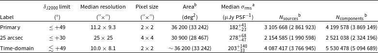
a
Uncertainties are reported from the $16\text{th}$
and
$16\text{th}$
and $84\text{th}$
percentiles.
$84\text{th}$
percentiles.
b
In parenthesis excluding the Galactic Plane ( $b\pm5^{\circ}$
).
$b\pm5^{\circ}$
).
We construct the catalogues by merging individual image source lists one-by-one, and cross-match sources in the incoming source list to the partially constructed catalogue. Sources in the partially constructed catalogue that match to a source in the incoming source lists with an angular separation, s, satisfying
 \begin{equation} s < \frac{1}{2} \left(\theta_{\text{M,1}} + \theta_{\text{M,2}}\right) \,\end{equation}
are considered duplicates, where $\theta_{\text{M,1}}$
is the PSF major axis of the source in the partially constructed catalogue and
$\theta_{\text{M,1}}$
is the PSF major axis of the source in the partially constructed catalogue and $ \theta_{\text{M,2}}$
is the PSF major axis of the source in the incoming source list. When a duplicate is found, the source that has the smallest separation from an image centre is kept. While constructing the catalogue, we also avoid sources within 2 arcmin of an image boundary to avoid cross-matching of extended sources that might be cut off at the edge of an image. The Gaussian components associated with the final set of sources are then collected into a separate component list.
$ \theta_{\text{M,2}}$
is the PSF major axis of the source in the incoming source list. When a duplicate is found, the source that has the smallest separation from an image centre is kept. While constructing the catalogue, we also avoid sources within 2 arcmin of an image boundary to avoid cross-matching of extended sources that might be cut off at the edge of an image. The Gaussian components associated with the final set of sources are then collected into a separate component list.
3. The catalogues
The catalogues produced as part of this data release are summarised in Table 1. These catalogues include (1) the primary catalogue comprising our best characterisation of each source at the observed and position-dependent resolution; (2) an auxiliary fixed 25-arcsec resolution catalogue, prepared similarly to the primary catalogue but with images convolved to a resolution of 25-arcsec; (3) an auxiliary time-domain catalogue, which includes all sources including those detected multiple times in adjacent images or duplicate observations of a particular field. The catalogues have identical columns, which are described in Appendix A. Note that in Appendix A. we also detail some changes to the columns and names used between the RACS-mid catalogues and the RACS-low catalogue. Tables A3 and A4 in Appendix A. also show example rows from the primary source and component catalogues, respectively. The catalogues are detailed further in the following sections.
3.1. The primary catalogue
The first catalogue is considered the primary catalogue and will be suitable for most general users. This catalogue covers the full region observed as part of RACS-mid and remains close to the angular resolution of the original RACS-mid images described in Reference DuchesnePaper IV. Construction of this catalogue begins with identifying adjacent fields, convolving to the lowest common resolution of that subset of fields, then forming full-sensitivity images as described in Section 2.2. Examples of the image quality is shown in Figs. 1 and 2 for a range of declinations, and Fig. 3 shows the variation of the PSF major [Fig. 3(i)] and minor [Fig. 3(ii)] axes as a function of declination for sources in the catalogue. The PSF for the primary catalogue is elliptical, and the major axis reaches 48.4 arcsec (at high declination) while the minor axis has a maximum of $ 18.9$
arcsec (at low declination).
$ 18.9$
arcsec (at low declination).
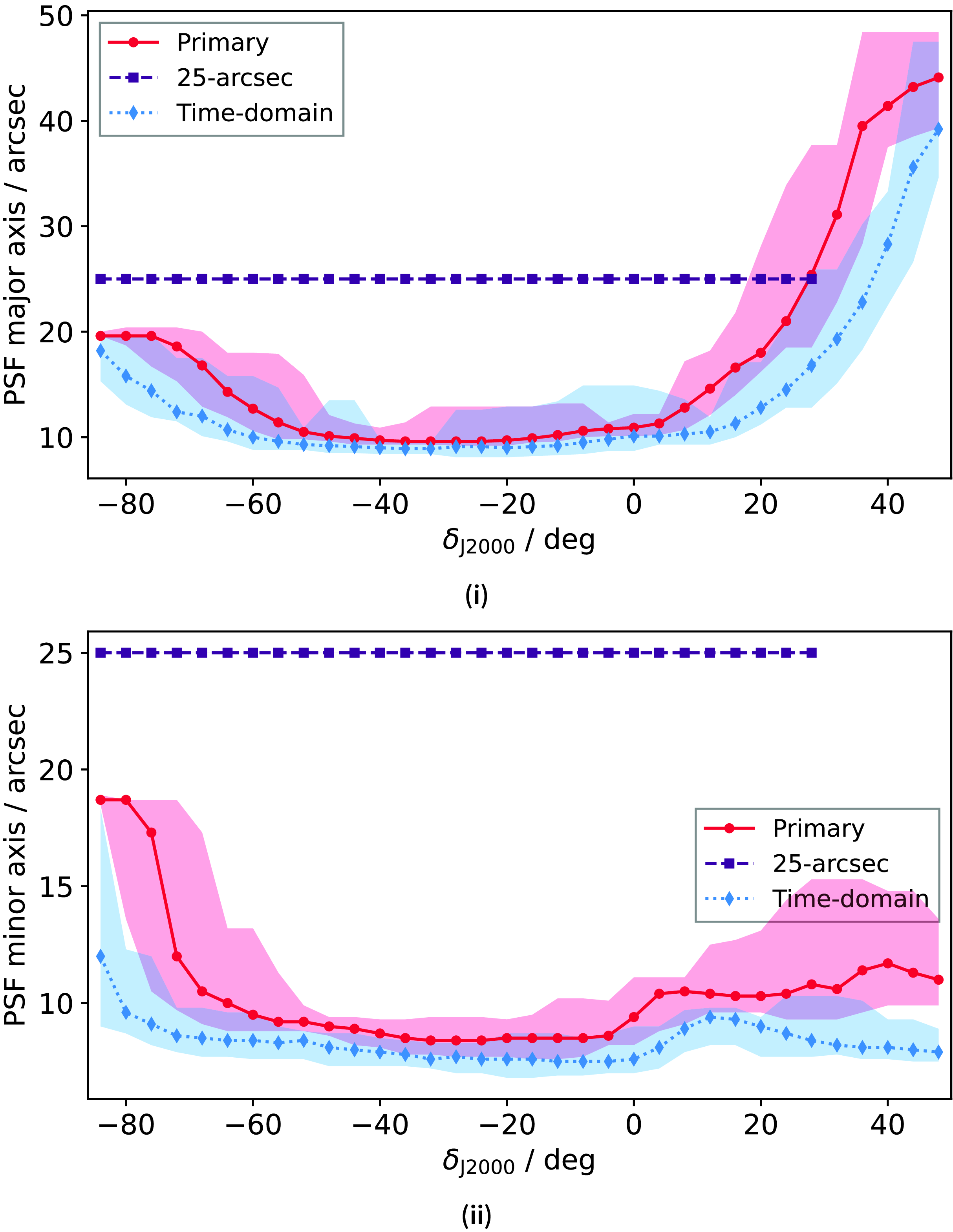
Figure 3. Variation of the major (i) and minor (ii) axes of the PSF over the RACS-mid primary catalogue (red), the 25-arcsec catalogue (purple), and the time-domain catalogue (blue). The filled markers are medians within 4-deg bins, and the shaded regions show the range of PSF axes within the given bins.
3.2. Auxiliary fixed-resolution, 25-arcsec catalogue
The second catalogue is an auxiliary ‘fixed-resolution’ catalogue, with a position-independent resolution of $25 \times 25$
arcsec
$25 \times 25$
arcsec $^2$
. Fig. 3 shows the 25-arcsec PSF compared to other catalogues’ PSF variation for reference. This catalogue is designed to match the RACS-low catalogue described by Reference HalePaper II, including the same resolution and sky coverage up to
$^2$
. Fig. 3 shows the 25-arcsec PSF compared to other catalogues’ PSF variation for reference. This catalogue is designed to match the RACS-low catalogue described by Reference HalePaper II, including the same resolution and sky coverage up to $\delta_{\text{J2000}} \leq +30^{\circ}$
.Footnote 6
$\delta_{\text{J2000}} \leq +30^{\circ}$
.Footnote 6
3.3. Auxiliary time-domain catalogue
As the previously mentioned catalogues are created after linearly mosaicking neighbouring observations, variable/transient radio sources may have their emission averaged between what may be two disjoint epochs. For many time-domain applications, it may be preferable to retain source detections and measurements at specific epochs. Searches for and characterisation of variable and transient sources have already been performed using individual images and sources lists from RACS-low (e.g. Leung et al. Reference Leung2021) and RACS-mid (e.g. Driessen et al. Reference Driessen, Heald, Duchesne, Murphy, Lenc, Leung and Moss2023; Gulati et al. Reference Gulati2023). To help enable further time-domain science, we provide another auxiliary catalogue for Stokes I that is simply the concatenation of source lists from the individual RACS-mid images. The individual images are not convolved prior to source-finding so they retain the original angular resolution. Fig. 3 shows the variation of the PSF at the locations of sources in the catalogue compared to the primary and 25-arcsec catalogues. As with the primary catalogue the PSF is elliptical and has a similar range of values. Sources that are detected in multiple images in overlap regions (i.e. duplicates) are not removed.
4. Analysis of the catalogues and images
In the following sections, we provide an analysis of the overall quality of the available catalogues and full-sensitivity image mosaics made. As the catalogue are created from the same original images, there is some redundancy to the following analysis and validation work. For consistency we show results for all catalogues where appropriate.

Figure 4. Median-binned HEALPix representation of the root-mean-square noise distributions of the primary catalogue (i), the 25-arcsec catalogue (ii), and the time-domain catalogue (iii). The black, dashed lines are drawn at Galactic latitudes $b \pm 5^{\circ}$
.
$b \pm 5^{\circ}$
.
4.1. Overall noise properties
The position-dependent rms noise properties of the images that are used for the three catalogues varies due to the difference in angular resolution and their overall construction. A local rms noise estimate is included for each source in the catalogue. Fig. 4 shows the rms noise median-binned using Hierarchical Equal Area isoLatitude Pixelation (HEALPix; Górski et al. Reference Górski, Hivon, Banday, Wandelt, Hansen, Reinecke and Bartelmann2005)Footnote 7 with $N_{\text{side}}=64$
corresponding to
$N_{\text{side}}=64$
corresponding to $\sim$ $55 \times 55$
arcmin
$55 \times 55$
arcmin $^{2}$
bins. The rms values are reported at the location of the source, so will on average be marginally elevated compared to off-source regions.
$^{2}$
bins. The rms values are reported at the location of the source, so will on average be marginally elevated compared to off-source regions.
The rms noise distribution of the primary catalogue [Fig. 4(i)] follows closely the median Stokes I noise per tile shown in Figure 24 of Reference DuchesnePaper IV, which was constructed by mosaicking position-dependent rms maps. The primary catalogue has a median rms noise of $\sigma_{\text{rms}} = 182_{-23}^{+41}$ $\mu$
Jy PSF
$\mu$
Jy PSF $^{-1}$
(with uncertainties derived from the
$^{-1}$
(with uncertainties derived from the $16\text{th}$
and
$16\text{th}$
and $84\text{th}$
percentiles of the rms noise distribution). This median rms noise is a decrease from the median rms noise reported over the original survey images reported in Reference DuchesnePaper IV due to the removal of the primary beam roll-off at the edge of convolved images. The larger spread in the distribution is due to the bias in local rms estimates taken from source locations, including the Galactic Plane and other areas of bright, extended sources. While not part of this data release, we note that the Stokes V images mosaicked and convolved in the same way achieve a median rms noise of
$84\text{th}$
percentiles of the rms noise distribution). This median rms noise is a decrease from the median rms noise reported over the original survey images reported in Reference DuchesnePaper IV due to the removal of the primary beam roll-off at the edge of convolved images. The larger spread in the distribution is due to the bias in local rms estimates taken from source locations, including the Galactic Plane and other areas of bright, extended sources. While not part of this data release, we note that the Stokes V images mosaicked and convolved in the same way achieve a median rms noise of $\sigma_{\text{rms},V} = 144_{-14}^{+20}$ $\mu$
Jy PSF
$\mu$
Jy PSF $^{-1}$
at the catalogued source positions.
$^{-1}$
at the catalogued source positions.

Figure 5. The number of PSF solid angles per source above $5\sigma_{\text{rms}}$
, binned as a function of declination for the RACS-mid primary and 25-arcsec catalogues, alongside equivalent products from RACS-low, the NVSS, SUMSS, and GLEAM. The shaded regions indicate maximum and minimum values corresponding to a varying PSF solid angle within declination bins.
$5\sigma_{\text{rms}}$
, binned as a function of declination for the RACS-mid primary and 25-arcsec catalogues, alongside equivalent products from RACS-low, the NVSS, SUMSS, and GLEAM. The shaded regions indicate maximum and minimum values corresponding to a varying PSF solid angle within declination bins.
The 25-arcsec catalogue [Fig. 4(ii)] has a median rms noise $\sigma_{\text{rms}} = 278_{-47}^{+68}$ $\mu$
Jy PSF
$\mu$
Jy PSF $^{-1}$
, generally showing an increase in rms noise over most of the sky due to the decrease in angular resolution. Of particular note is an additional increase in noise near the celestial equator, corresponding to residuals from the poorer equatorial PSF becoming significant after convolution to the lower 25-arcsec resolution. Convolving the images to the lower
$^{-1}$
, generally showing an increase in rms noise over most of the sky due to the decrease in angular resolution. Of particular note is an additional increase in noise near the celestial equator, corresponding to residuals from the poorer equatorial PSF becoming significant after convolution to the lower 25-arcsec resolution. Convolving the images to the lower $25\times25$
arcsec
$25\times25$
arcsec $^{2}$
PSF also results in a general loss of information in the images, translating to an overall increase in the image rms noise. The difference in the median Stokes I and Stokes V noise (
$^{2}$
PSF also results in a general loss of information in the images, translating to an overall increase in the image rms noise. The difference in the median Stokes I and Stokes V noise ( $\sigma_{\text{rms},V} = 167_{-17}^{+23}$ $\mu$
Jy PSF
$\mu$
Jy PSF $^{-1}$
) is comparatively larger than for the primary catalogue, suggesting another contribution to the increase in noise is the increase in classical source confusion at this lower resolution (Condon Reference Condon1974) though the 25-arcsec catalogue is not confusion-limited (see Section 4.2).
$^{-1}$
) is comparatively larger than for the primary catalogue, suggesting another contribution to the increase in noise is the increase in classical source confusion at this lower resolution (Condon Reference Condon1974) though the 25-arcsec catalogue is not confusion-limited (see Section 4.2).
Finally, the time-domain catalogue [Fig. 4(iii)] features increased noise at the boundaries between fields due to overlapping uncorrected primary beam roll-off. The remainder of the survey area has similar position-dependent noise characteristics to the primary catalogue due to the similarities towards the image centres. The median rms noise, $\sigma_{\text{rms}} = 203_{-33}^{+140}$ $\mu$
Jy PSF
$\mu$
Jy PSF $^{-1}$
is closer to the tile median reported in Reference DuchesnePaper IV with an increase in spread due to bias in the sampled noise locations (i.e. at the locations of sources).
$^{-1}$
is closer to the tile median reported in Reference DuchesnePaper IV with an increase in spread due to bias in the sampled noise locations (i.e. at the locations of sources).
4.2. Classical source confusion
While we do not expect even the deeper 10-hr images from ASKAP to become limited by classical source confusion noise at 1.4 GHz (assuming a $10\times10$
arcsec
$10\times10$
arcsec $^{2}$
PSF; Condon et al. Reference Condon2012), as this noise is a function of PSF solid angle [
$^{2}$
PSF; Condon et al. Reference Condon2012), as this noise is a function of PSF solid angle [ $\Omega_{\text{PSF}} = \pi\theta_{\text{M}}\theta_{\text{m}}/\left(4\ln{2}\right)$
] it is worth considering a possible limit given the variable PSFs of the RACS-mid catalogues. The number of PSF solid angles per source above some flux density threshold is often used as an estimate of the severity of confusion (e.g. Cohen 2004; Condon et al. Reference Condon2012; Heywood et al. Reference Heywood2016), with values of order
$\Omega_{\text{PSF}} = \pi\theta_{\text{M}}\theta_{\text{m}}/\left(4\ln{2}\right)$
] it is worth considering a possible limit given the variable PSFs of the RACS-mid catalogues. The number of PSF solid angles per source above some flux density threshold is often used as an estimate of the severity of confusion (e.g. Cohen 2004; Condon et al. Reference Condon2012; Heywood et al. Reference Heywood2016), with values of order $\lesssim$
10 indicating that the images are limited in sensitivity by confusion.
$\lesssim$
10 indicating that the images are limited in sensitivity by confusion.
Fig. 5 shows the number of PSF solid angles per source above $5\sigma_{\text{rms}}$
(
$5\sigma_{\text{rms}}$
( $N_\Omega / N_{\text{sources}}$
) binned as a function of declination, excluding the area covering Galactic latitudes of
$N_\Omega / N_{\text{sources}}$
) binned as a function of declination, excluding the area covering Galactic latitudes of $|b|<10^{\circ}$
. We also show the equivalent product with the same threshold for some other surveys with largely contiguous sky coverage: the NVSS (Condon et al. Reference Condon, Cotton, Greisen, Yin, Perley, Taylor and Broderick1998) with a
$|b|<10^{\circ}$
. We also show the equivalent product with the same threshold for some other surveys with largely contiguous sky coverage: the NVSS (Condon et al. Reference Condon, Cotton, Greisen, Yin, Perley, Taylor and Broderick1998) with a $45\times45$
arcsec
$45\times45$
arcsec $^2$
PSF, the Sydney University Molonglo Sky Survey (SUMSS; Bock et al. Reference Bock, Large and Sadler1999; Mauch et al. Reference Mauch, Murphy, Buttery, Curran, Hunstead, Piestrzynski, Robertson and Sadler2003) with a position-dependent
$^2$
PSF, the Sydney University Molonglo Sky Survey (SUMSS; Bock et al. Reference Bock, Large and Sadler1999; Mauch et al. Reference Mauch, Murphy, Buttery, Curran, Hunstead, Piestrzynski, Robertson and Sadler2003) with a position-dependent $45\times45/\text{sin}\lvert\delta_{\text{J2000}}\rvert$
arcsec
$45\times45/\text{sin}\lvert\delta_{\text{J2000}}\rvert$
arcsec $^2$
PSF, and the Galactic and Extragalactic All-sky MWAFootnote 8 survey (GLEAM; Wayth et al. Reference Wayth2015) extragalactic catalogue (Hurley-Walker et al. Reference Hurley-Walker2017) with a position-dependent PSF major axis that varies between
$^2$
PSF, and the Galactic and Extragalactic All-sky MWAFootnote 8 survey (GLEAM; Wayth et al. Reference Wayth2015) extragalactic catalogue (Hurley-Walker et al. Reference Hurley-Walker2017) with a position-dependent PSF major axis that varies between $\sim$
128–240 arcsec and minor axis that varies between
$\sim$
128–240 arcsec and minor axis that varies between $\sim$
122–173 arcsec at 200 MHz. Note we do not include the RACS-mid time-domain catalogue as the overlapping observations artificially increase the source density and are not reflective of the actual images used. The shaded regions in Fig. 5 show the range of values within a declination bin for surveys with variable PSFs.
$\sim$
122–173 arcsec at 200 MHz. Note we do not include the RACS-mid time-domain catalogue as the overlapping observations artificially increase the source density and are not reflective of the actual images used. The shaded regions in Fig. 5 show the range of values within a declination bin for surveys with variable PSFs.
Despite the elongated PSF of the primary catalogue at high declination, the solid angle remains small due to the high ellipticity of the PSF ( $\theta_{\text{M}}/\theta_{\text{m}} \lesssim 4.7$
). The number of PSF solid angles per source is thus sufficiently high that we do not consider classical source confusion to be the predominant noise in the RACS-mid images and subsequent catalogues. We note that the 25-arcsec catalogue generally has a larger PSF solid angle than the primary catalogue (except in seven of the full-sensitivity images used for the primary catalogue) and so is overall more affected, though still not limited by classical source confusion.
$\theta_{\text{M}}/\theta_{\text{m}} \lesssim 4.7$
). The number of PSF solid angles per source is thus sufficiently high that we do not consider classical source confusion to be the predominant noise in the RACS-mid images and subsequent catalogues. We note that the 25-arcsec catalogue generally has a larger PSF solid angle than the primary catalogue (except in seven of the full-sensitivity images used for the primary catalogue) and so is overall more affected, though still not limited by classical source confusion.
4.3. Source density
Fig. 6 shows the HEALPix-binned ( $N_{\text{side}}=64$
,
$N_{\text{side}}=64$
, $\sim 55 \times 55$
arcmin
$\sim 55 \times 55$
arcmin $^{2}$
) source and component density across the sky for the primary catalogue [Fig. 6(i) and 6(ii)], the 25-arcsec catalogue [Fig. 6(iii) and 6(iv)], and the time-domain catalogue [Fig. 6(v) and 6(vi)]. The average source density across the primary catalogue is
$^{2}$
) source and component density across the sky for the primary catalogue [Fig. 6(i) and 6(ii)], the 25-arcsec catalogue [Fig. 6(iii) and 6(iv)], and the time-domain catalogue [Fig. 6(v) and 6(vi)]. The average source density across the primary catalogue is $\sim$
86 deg
$\sim$
86 deg $^{-2}$
, over the catalogued area of
$^{-2}$
, over the catalogued area of $\sim$ $36\,200$
deg
$36\,200$
deg $^{2}$
. The 25-arcsec catalogue has a source density of
$^{2}$
. The 25-arcsec catalogue has a source density of $\sim$
70 deg
$\sim$
70 deg $^{-2}$
(coverage
$^{-2}$
(coverage $\sim 30\,900$
deg
$\sim 30\,900$
deg $^{2}$
) and the time-domain catalogue has a source density of
$^{2}$
) and the time-domain catalogue has a source density of $\sim$
113 deg
$\sim$
113 deg $^{-2}$
(coverage
$^{-2}$
(coverage $\sim$ $36\,200$
deg
$36\,200$
deg $^{2}$
, though note that by construction there are many duplicate sources in the time-domain catalogue).
$^{2}$
, though note that by construction there are many duplicate sources in the time-domain catalogue).
In the primary and 25-arcsec catalogues the Galactic Plane features a lower density of sources, largely due to higher noise on multiple scales. This is a combination of both the real extended sources and the artefacts on multiple angular scales from the poor modelling of the real extended sources. A similar decrease in source density is not as obvious in the time-domain catalogue due to the double-counting of sources in overlap regions. We also see a decrease in source density at the celestial equator corresponding to a reduction in image sensitivity. This is most prominent in the 25-arcsec catalogue. The component density of all three catalogues is higher than the source density, corresponding to the resolved sources being modelled with multiple Gaussian components by PyBDSF. Smaller-scale low-density regions can be seen around other bright sources, though generally restricted to the 1.2 degree radius left from peeling described in Reference DuchesnePaper IV. The regions in all three catalogues around $\delta_{\text{J2000}} \approx -75$
show significantly higher average source density caused by the large overlap in adjacent observations where the Celestial tiling changes to cover the South Celestial Pole. The time-domain catalogue features increased source density regions with duplicate observations as we do not remove the duplicated sources.
$\delta_{\text{J2000}} \approx -75$
show significantly higher average source density caused by the large overlap in adjacent observations where the Celestial tiling changes to cover the South Celestial Pole. The time-domain catalogue features increased source density regions with duplicate observations as we do not remove the duplicated sources.
In Fig. 7 we also show the source density, binned as a function of declination for six flux density limits (1, 2, 3, 4, 5, and 10 mJy) with the Galactic Plane excluded. The features described for the HEALPix maps are clear in the 1- and 2-mJy flux density populations but largely begin to disappear for the brighter source populations with the 10-mJy source density showing no variation as a function of declination. The exception to this is the time-domain catalogue, for which the 10-mJy population still shows variation in source density as a function of declination—a consequence of including duplicated source entries.
4.4. The fraction of unresolved sources
For certain comparisons to external surveys, it is generally preferable to consider isolated and unresolved sources to avoid biases introduced by differences in (u,v) coverage, and by extension angular resolution. While some comparison could be done for resolved/extended radio sources, comparison in that case becomes more heavily affected by differences in (u,v) coverage and frequency.

Figure 6. HEALPix representation of the source and component density of the primary catalogue [(i) and (ii)], the 25-arcsec catalogue [(iii) and (iv)], and the time-domain catalogue [(v) and (vi)]. The black, dashed lines are drawn at Galactic latitudes $b \pm 5^{\circ}$
. Regions with no sources are coloured grey. The colourscales are kept the same to highlight the differences in source/component densities.
$b \pm 5^{\circ}$
. Regions with no sources are coloured grey. The colourscales are kept the same to highlight the differences in source/component densities.
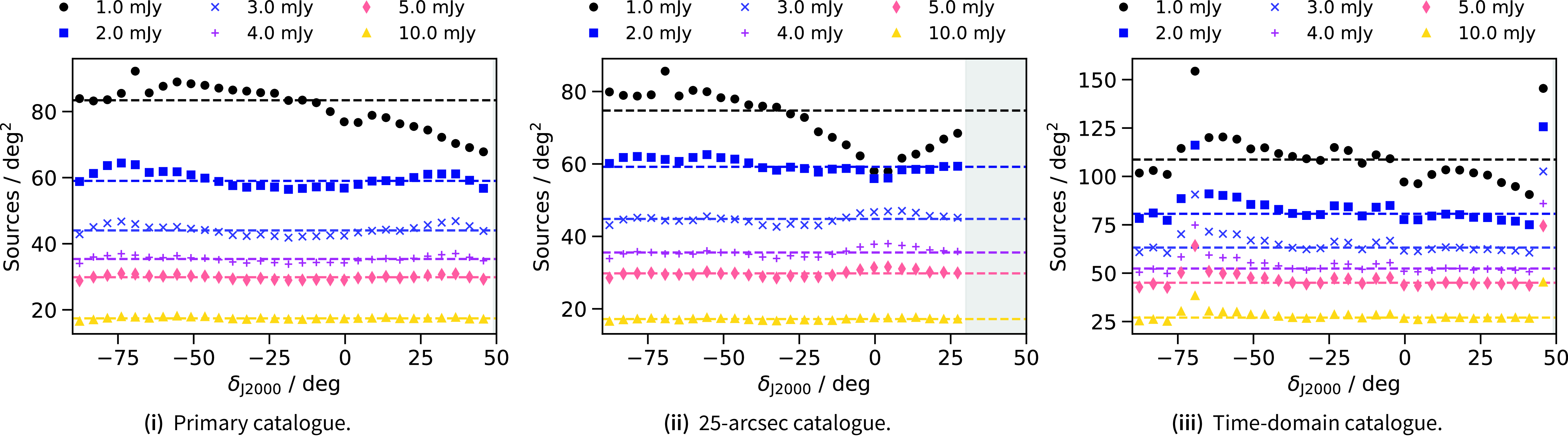
Figure 7. Source density as a function of declination for six flux density limits ([1, 2, 3, 4, 5, 10] mJy) for the primary catalogue (i), the 25-arcsec catalogue (ii), and the time-domain catalogue (iii). Dashed lines correspond to median source densities for the associated flux density limit. The grey, shaded region in (ii) is not covered in the 25-arcsec catalogue.
To create an unresolved subset of the primary catalogue and two auxiliary catalogues, we opt to follow the procedure outlined in Section 5.2.1 of Reference HalePaper II following similar methods employed by, for example, Bondi et al. (Reference Bondi, Ciliegi and Schinnerer2008), Smolčić et al. (Reference Smolčić2017a), Shimwell et al. (Reference Shimwell2019). Firstly, this involves assuming the ratio of integrated flux density, $S_{\text{int}}$
, and peak flux density,
$S_{\text{int}}$
, and peak flux density, $S_{\text{peak}}$
, is close to unity for an unresolved source. In practice,
$S_{\text{peak}}$
, is close to unity for an unresolved source. In practice, $S_{\text{int}}/S_{\text{peak}} > 1$
for a variety of reasons, including: source positions may move during the observation or due to mosaicking adjacent images with small astrometric offsets resulting in a blurred source in final images; self-calibration processes may pull sources in different directions in adjacent beam images (see Section 3.4.3 in Reference McConnellPaper I or Section 3.7.1 in Reference DuchesnePaper IV), resulting in blurring of the source. In these situations integrated flux density is generally preserved and peak flux density decreases. Other factors such as as bandwidth or time smearing cause similar problems, which for RACS-mid can be up to
$S_{\text{int}}/S_{\text{peak}} > 1$
for a variety of reasons, including: source positions may move during the observation or due to mosaicking adjacent images with small astrometric offsets resulting in a blurred source in final images; self-calibration processes may pull sources in different directions in adjacent beam images (see Section 3.4.3 in Reference McConnellPaper I or Section 3.7.1 in Reference DuchesnePaper IV), resulting in blurring of the source. In these situations integrated flux density is generally preserved and peak flux density decreases. Other factors such as as bandwidth or time smearing cause similar problems, which for RACS-mid can be up to $\sim$
2–4 % reduction towards the edges of primary beam mainlobe, depending on pointing. The blurring, or smearing, of sources more heavily affects those in the low-SNR regime and low-SNR sources may also be pushed to
$\sim$
2–4 % reduction towards the edges of primary beam mainlobe, depending on pointing. The blurring, or smearing, of sources more heavily affects those in the low-SNR regime and low-SNR sources may also be pushed to $S_{\text{int}}/S_{\text{peak}} < 1$
due to image noise and uncertainty while fitting Gaussian components to sources.
$S_{\text{int}}/S_{\text{peak}} < 1$
due to image noise and uncertainty while fitting Gaussian components to sources.
As in Reference HalePaper II, we begin by assuming that unresolved sources sit within an envelope defined by
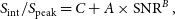 \begin{equation} S_{\text{int}}/S_{\text{peak}} = C + A\times \text{SNR}^{B} \,, \end{equation}
where C is an estimate of the median $S_{\text{int}}/S_{\text{peak}}$
in the high-SNR regime unique to each catalogue as it will depend on the average PSF. A and B are found by fitting Equation (3) as in Reference HalePaper II, after binning values below C and obtaining the
$S_{\text{int}}/S_{\text{peak}}$
in the high-SNR regime unique to each catalogue as it will depend on the average PSF. A and B are found by fitting Equation (3) as in Reference HalePaper II, after binning values below C and obtaining the $100-95{\text{th}}$
percentile in each bin.
$100-95{\text{th}}$
percentile in each bin.
Fig. 8 shows the ratio $S_{\text{int}}/S_{\text{peak}}$
as a function of SNR for single-component sources, along with the fitted envelopes highlighting the resolved sources for each of the three catalogues. The percentage of unresolved sources naturally increases as the catalogue resolution decreases, ranging from
$S_{\text{int}}/S_{\text{peak}}$
as a function of SNR for single-component sources, along with the fitted envelopes highlighting the resolved sources for each of the three catalogues. The percentage of unresolved sources naturally increases as the catalogue resolution decreases, ranging from $48.4\%$
in the primary catalogue to
$48.4\%$
in the primary catalogue to $58.7\%$
in the 25-arcsec catalogue. Despite the lower rms noise in the RACS-mid data compared to RACS-low, we find a higher fraction of unresolved sources (cf.
$58.7\%$
in the 25-arcsec catalogue. Despite the lower rms noise in the RACS-mid data compared to RACS-low, we find a higher fraction of unresolved sources (cf. $\sim$
40% for RACS-low; Reference HalePaper II). We suggest this is largely due to the loss in sensitivity to extended sources in the RACS-mid images, and the lower number of resolved sources in the 25-arcsec catalogue is further evidence of this.
$\sim$
40% for RACS-low; Reference HalePaper II). We suggest this is largely due to the loss in sensitivity to extended sources in the RACS-mid images, and the lower number of resolved sources in the 25-arcsec catalogue is further evidence of this.
Identifying unresolved/resolved sources in this way also highlights a subset of the catalogued sources that fall both below $ S_{\text{int}}/S_{\text{peak}} < 1$
and
$ S_{\text{int}}/S_{\text{peak}} < 1$
and $S_{\text{int}}/S_{\text{peak}} < C + A\times \text{SNR}^{B}$
(i.e. below the envelope). Such sources are unlikely to be real and may be spurious source-finder detections or artefacts. We therefore add a column in each catalogue called Flag which can be one of the following:
$S_{\text{int}}/S_{\text{peak}} < C + A\times \text{SNR}^{B}$
(i.e. below the envelope). Such sources are unlikely to be real and may be spurious source-finder detections or artefacts. We therefore add a column in each catalogue called Flag which can be one of the following:
Flag = 0 An unresolved source, satisfying:
 \begin{equation} S_{\text{int}} / S_{\text{peak}} > \left(C + A\times \text{SNR}^{B}\right) \,, \end{equation}
or
 \begin{equation} 1 \leq S_{\text{int}} / S_{\text{peak}} < \left(C - A\times \text{SNR}^{B}\right) \, .\end{equation}
The second condition covers high-SNR sources that have $S_{\text{int}}/S_{\text{peak}}$
below the median
$S_{\text{int}}/S_{\text{peak}}$
below the median $S_{\text{int}}/S_{\text{peak}}$
but are not spurious detections. The requirement to include such sources suggests the fitted envelope is not a completely accurate in determining unresolved sources.
$S_{\text{int}}/S_{\text{peak}}$
but are not spurious detections. The requirement to include such sources suggests the fitted envelope is not a completely accurate in determining unresolved sources.
Flag = 1 A resolved source, satisfying:
 \begin{equation} S_{\text{int}} / S_{\text{peak}} > \left(C - A\times \text{SNR}^{B}\right) \, .\end{equation}
Flag = 2 A spurious source, not satisfying the above (i.e. $S_{\text{int}}/S_{\text{peak}}$
below 1 and below the envelope), likely to be an artefact.
$S_{\text{int}}/S_{\text{peak}}$
below 1 and below the envelope), likely to be an artefact.
4.5. Reliability
Following Reference HalePaper II, we investigate the reliability of our images and source-finding by quantifying the number of sources detected by PyBDSF below $-5\sigma_{\text{rms}}$
. We assume the noise is symmetric in the image and define the reliability as
$-5\sigma_{\text{rms}}$
. We assume the noise is symmetric in the image and define the reliability as $1-N_{\text{negative}}/N$
, where N is the number of sources found above
$1-N_{\text{negative}}/N$
, where N is the number of sources found above $5\sigma_{\text{rms}}$
and
$5\sigma_{\text{rms}}$
and $N_{\text{negative}}$
are sources detected below
$N_{\text{negative}}$
are sources detected below $-5\sigma_{\text{rms}}$
. We repeat source-finding on all images (used for the primary catalogue and the two auxiliary catalogues) after multiplying the images by
$-5\sigma_{\text{rms}}$
. We repeat source-finding on all images (used for the primary catalogue and the two auxiliary catalogues) after multiplying the images by $-1$
and setting the source-finding threshold to
$-1$
and setting the source-finding threshold to $5\sigma_{\text{rms}}$
as in the normal source-finding procedure. Due to the choice of box size for rms calculations, for many images no sources are found in these inverted images. The source lists generated from the inverted images are then merged following the same process used for each catalogue. The source flags outlined in Section 4.4 are also added assuming the same criteria for each catalogue. Fig. 9(i)–9(iii) show flux density histograms of sources detected in the RACS-mid catalogues in both the normal catalogues and negative catalogues.
$5\sigma_{\text{rms}}$
as in the normal source-finding procedure. Due to the choice of box size for rms calculations, for many images no sources are found in these inverted images. The source lists generated from the inverted images are then merged following the same process used for each catalogue. The source flags outlined in Section 4.4 are also added assuming the same criteria for each catalogue. Fig. 9(i)–9(iii) show flux density histograms of sources detected in the RACS-mid catalogues in both the normal catalogues and negative catalogues.
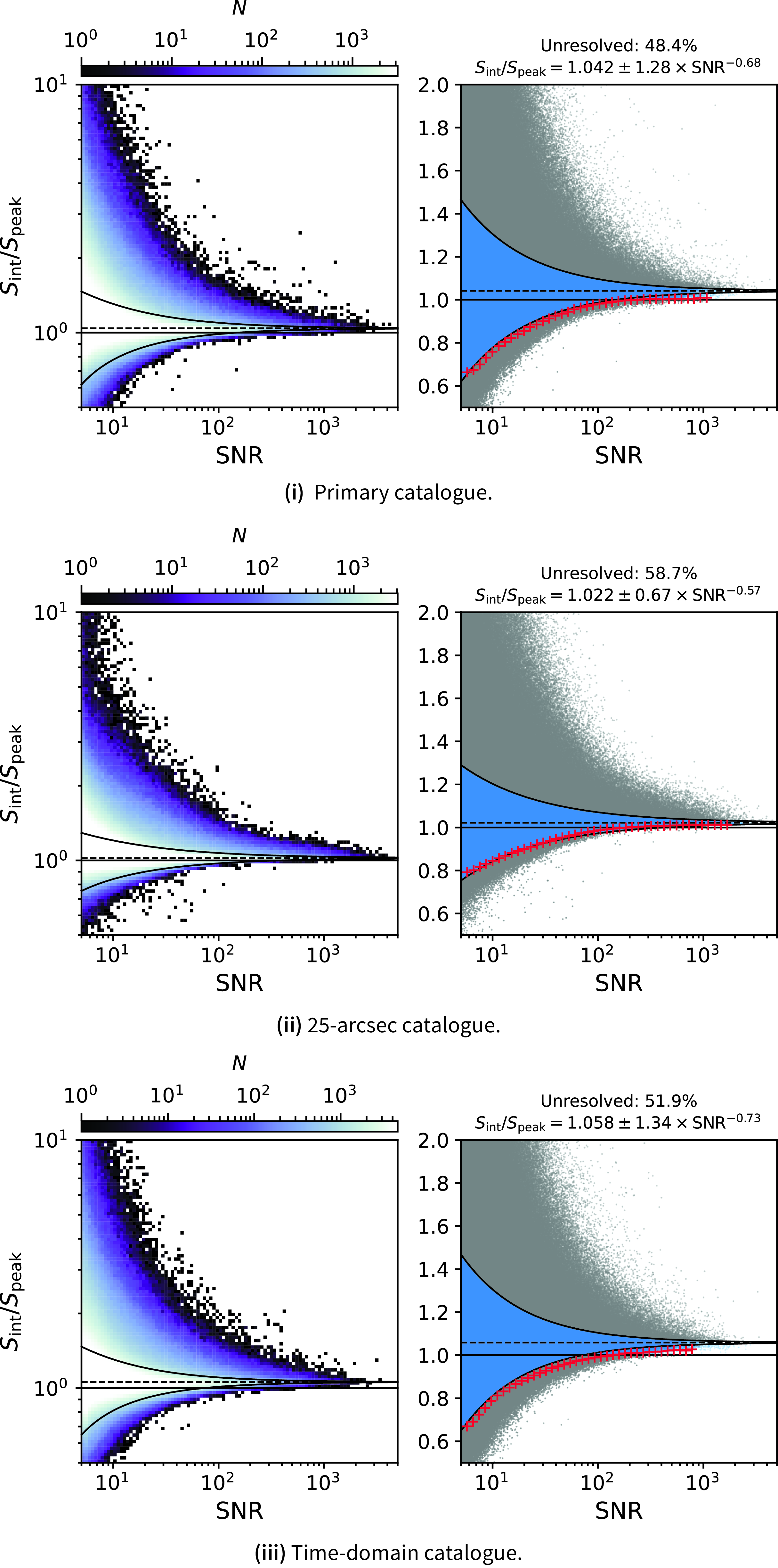
Figure 8. The ratio of integrated flux density ( $S_{\text{int}}$
) to peak flux density (
$S_{\text{int}}$
) to peak flux density ( $S_{\text{peak}}$
) as a function of signal-to-noise ratio (
$S_{\text{peak}}$
) as a function of signal-to-noise ratio ( $\text{SNR} = S_{\text{peak}} / \sigma_{\text{rms}}$
). The left panels show binned 2D histograms of the sources while the right panel shows a zoomed-in region with unresolved sources coloured blue. Red crosses in the right panel indicate the binned values used to fit the lower envelope. The lower and upper envelope are drawn as solid black lines, and the median
$\text{SNR} = S_{\text{peak}} / \sigma_{\text{rms}}$
). The left panels show binned 2D histograms of the sources while the right panel shows a zoomed-in region with unresolved sources coloured blue. Red crosses in the right panel indicate the binned values used to fit the lower envelope. The lower and upper envelope are drawn as solid black lines, and the median $S_{\text{int}}/S_{\text{peak}}$
value is shown as a black, dashed line. The single solid, black horizontal line indicates
$S_{\text{int}}/S_{\text{peak}}$
value is shown as a black, dashed line. The single solid, black horizontal line indicates $S_{\text{int}}/S_{\text{peak}} = 1$
.
$S_{\text{int}}/S_{\text{peak}} = 1$
.
Fig. 10(i)–10(iii) show an estimate of the catalogues’ reliability for sources outside of the Galactic Plane ( $|b| > 5^{\circ}$
), binned as a function of declination for a range of flux density cuts (including 1, 5, and 10 mJy). We find that reliability is not constant in declination. In Table 2 we report median reliability as a percentage of sources without a negative counterpart for the given flux density limits and the full catalogues. For sources outside of the Galactic Plane, we find overall reliability of 99.28 (99.37)%, 99.88 (99.88)%, and 98.68 (98.86)%, for the primary, 25-arcsec, and time-domain catalogues, respectively, with (and without) the ‘spurious’ sources included. The time-domain catalogue shows the least reliability, which is a consequence of including the high-noise regions at the edges of images. Conversely, the 25-arcsec catalogue has least number of negative sources and closely reflects the reliability of the RACS-low catalogue, also at 25-arcsec (cf.
$|b| > 5^{\circ}$
), binned as a function of declination for a range of flux density cuts (including 1, 5, and 10 mJy). We find that reliability is not constant in declination. In Table 2 we report median reliability as a percentage of sources without a negative counterpart for the given flux density limits and the full catalogues. For sources outside of the Galactic Plane, we find overall reliability of 99.28 (99.37)%, 99.88 (99.88)%, and 98.68 (98.86)%, for the primary, 25-arcsec, and time-domain catalogues, respectively, with (and without) the ‘spurious’ sources included. The time-domain catalogue shows the least reliability, which is a consequence of including the high-noise regions at the edges of images. Conversely, the 25-arcsec catalogue has least number of negative sources and closely reflects the reliability of the RACS-low catalogue, also at 25-arcsec (cf. $\sim$ $99.7$
% reliability reported in Reference HalePaper II). We find that the primary catalogue suffers from its increased angular resolution, where smaller-scale, low-significance artefacts (not present in the 25-arcsec images) are harder to avoid during rms-thresholding and source-finding. As the reliability is lowest at declinations where the PSF is smallest, it is clear the angular resolution plays a significant role in affecting the reliability of the source-finding and catalogues.
$99.7$
% reliability reported in Reference HalePaper II). We find that the primary catalogue suffers from its increased angular resolution, where smaller-scale, low-significance artefacts (not present in the 25-arcsec images) are harder to avoid during rms-thresholding and source-finding. As the reliability is lowest at declinations where the PSF is smallest, it is clear the angular resolution plays a significant role in affecting the reliability of the source-finding and catalogues.
We repeat this comparison for sources within the Galactic Plane ( $|b| < 5^{\circ}$
), with medians reported in Table 2 and in Fig. 10(iv)–10(vi). Generally there is an increase in negative sources detected in the Galactic Plane. This is most notable in the 25-arcsec catalogue, where reliability gets worse for brighter sources. This is due to artefacts caused by unmodelled (and poorly modelled) extended emission. When convolved to 25-arcsec, these artefacts become significant with respect to the background noise and the source-finder treats them as real sources. We suggest users of the 25-arcsec catalogue (and 25-arcsec images) be cautious when selecting sources in the Galactic Plane.
$|b| < 5^{\circ}$
), with medians reported in Table 2 and in Fig. 10(iv)–10(vi). Generally there is an increase in negative sources detected in the Galactic Plane. This is most notable in the 25-arcsec catalogue, where reliability gets worse for brighter sources. This is due to artefacts caused by unmodelled (and poorly modelled) extended emission. When convolved to 25-arcsec, these artefacts become significant with respect to the background noise and the source-finder treats them as real sources. We suggest users of the 25-arcsec catalogue (and 25-arcsec images) be cautious when selecting sources in the Galactic Plane.
4.6. Completeness
To estimate the completeness of the RACS-mid catalogues, we follow Reference HalePaper II and inject a realistic sky model into the individual images after subtracting the Gaussian components found and modelled by PyBDSF. For this purpose, we use the semi-empirical sky model from the SKA Simulated Skies project (Wilman et al. Reference Wilman2008; Levrier et al. Reference Levrier, Wilman, Obreschkow, Kloeckner, Heywood and Rawlings2009). We use a base sky model that covers a 100 deg $^{2}$
region including sources considered both resolved and unresolved at the angular resolution of the RACS-mid data. For each image, we generate five separate sub-sky models by randomising positions of sources from the 100-deg
$^{2}$
region including sources considered both resolved and unresolved at the angular resolution of the RACS-mid data. For each image, we generate five separate sub-sky models by randomising positions of sources from the 100-deg $^{2}$
sky model. We clip the sub-sky models at
$^{2}$
sky model. We clip the sub-sky models at $3\sigma_{\text{rms}}$
and at
$3\sigma_{\text{rms}}$
and at $2 \times S_{\text{max}}$
where
$2 \times S_{\text{max}}$
where $S_{\text{max}}$
is the maximum flux density of real sources in the image. We do not expect full recovery of sources at the brightest flux densities, as the brightest sources are typically extended at the RACS-mid resolution (e.g. Perley & Butler Reference Perley and Butler2017) and RACS-mid has poorer sensitivity to extended sources (see e.g. Section 3.5 and Figure 26 in Reference DuchesnePaper IV). The semi-empirical SKA sky model may not be accurate below
$S_{\text{max}}$
is the maximum flux density of real sources in the image. We do not expect full recovery of sources at the brightest flux densities, as the brightest sources are typically extended at the RACS-mid resolution (e.g. Perley & Butler Reference Perley and Butler2017) and RACS-mid has poorer sensitivity to extended sources (see e.g. Section 3.5 and Figure 26 in Reference DuchesnePaper IV). The semi-empirical SKA sky model may not be accurate below $\sim$ $0.1$
mJy (e.g. Smolčić et al. Reference Smolčić2017a; Hale et al. Reference Hale2023), which is generally below the rms noise in the RACS-mid images. The low flux density limit still allows sources below our detection thresholds to be modelled, but are typically above
$0.1$
mJy (e.g. Smolčić et al. Reference Smolčić2017a; Hale et al. Reference Hale2023), which is generally below the rms noise in the RACS-mid images. The low flux density limit still allows sources below our detection thresholds to be modelled, but are typically above $0.1$
mJy. This provides a total sub-sky model flux density of
$0.1$
mJy. This provides a total sub-sky model flux density of $\sim$
150 Jy for each image. We do not distinguish between unresolved and resolved sources for these tests.
$\sim$
150 Jy for each image. We do not distinguish between unresolved and resolved sources for these tests.
The sub-sky models are injected onto model images and then restored in a similar way to normal imaging: the model is first convolved with the image PSF then the convolved model is added to the residual map. We use PyBDSF to source-find these model-injected images using the same settings as we used for the real images. The individual output source lists are then cross-matched to the original sub-sky model catalogues for each image independently before concatenation. For this purpose we use the source list output by PyBDSF rather than the component list. This process is done separately for all image set used to generate the catalogues.

Figure 9. Histograms of the negative (pink) and positive (blue) components found over the survey images used in the primary (i), 25-arcsec (ii), and time-domain (iii) catalogues.
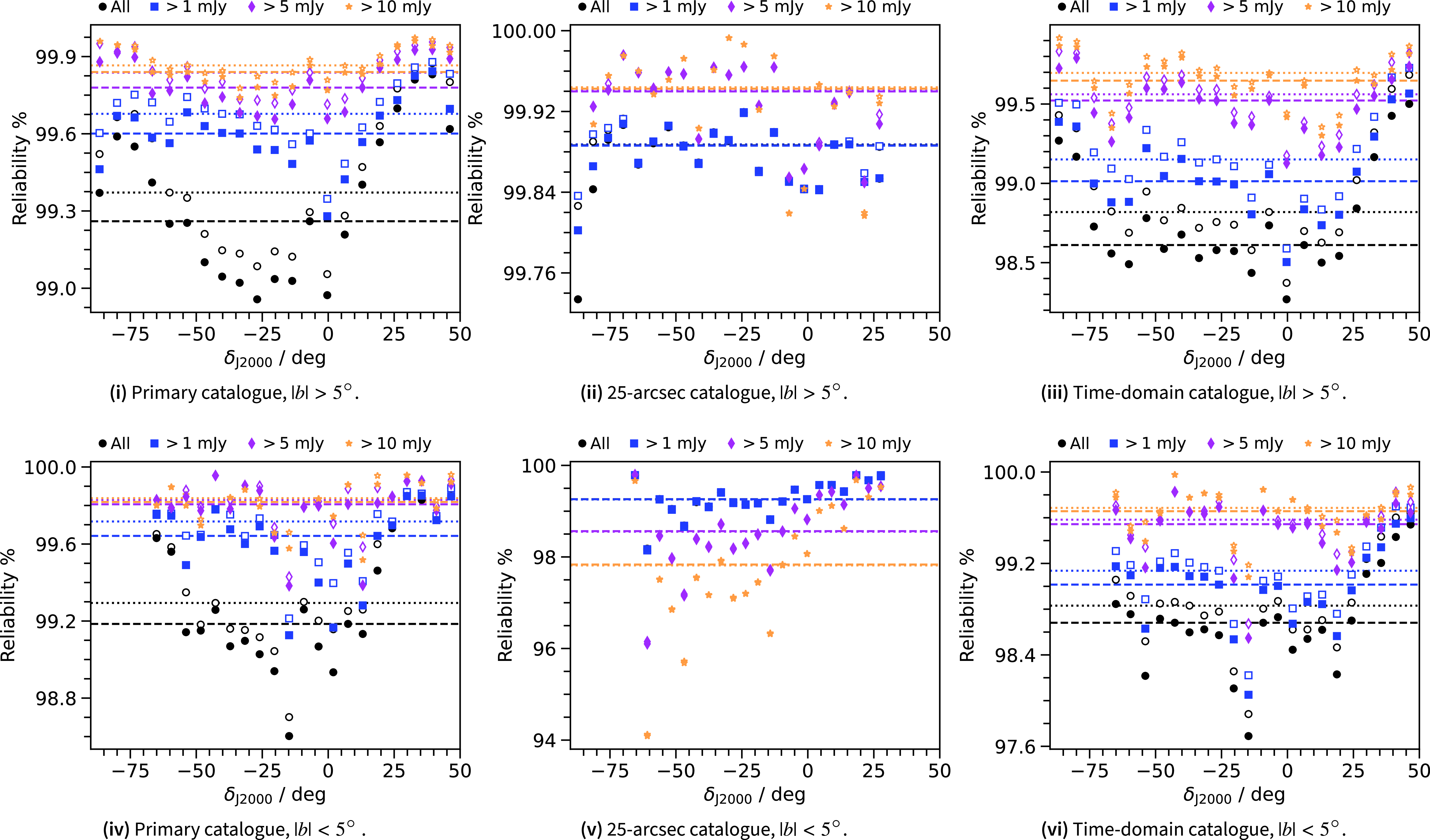
Figure 10. Reliability for the three catalogues as a function of declination for different flux density cuts. Empty markers correspond to the subsample that excludes the Flag = 2 ‘spurious’ sources. Horizontal lines correspond to medians for each flux density limit (dashed lines for the full samples, and dotted lines for the subsample). Top row. [(i)–(iii)] Sources outside of the Galactic Plane ( $|b|>5^{\circ}$
). Bottom row. [(iv)–(vi)] Sources within the Galactic Plane (
$|b|>5^{\circ}$
). Bottom row. [(iv)–(vi)] Sources within the Galactic Plane ( $|b|<5^{\circ}$
). Note all plots show a different y-axis scale to highlight different declination-dependent features.
$|b|<5^{\circ}$
). Note all plots show a different y-axis scale to highlight different declination-dependent features.
In Fig. 11(i)–11(iii) we show the fraction of sources that are cross-matched to the input sky model after source-finding the three RACS-mid catalogues. As in Reference HalePaper II, the detection fraction is calculated in logarithmically sampled flux density bins, and we show both cumulative (orange line) and independent (blue line) detection fractions with 50% and 95% detection fractions highlighted. The detection fractions at 50% and 95% are higher than in RACS-low for the primary catalogue and conversely lower for for the 25-arcsec catalogue. The drop in detection fraction for the 25-arcsec catalogue is on account of increased blending of sources at the lower resolution of the 25-arcsec catalogue.
Fig. 11(iv)–11(vi) show the completeness of each catalogue as a function of flux density. This is defined as the binned ratio of recovered flux density as a function of flux density. The primary catalogue is found to be 50% complete at 1.1 mJy and 95% complete at 1.6 mJy while we find 1.7 and 2.5 mJy completeness (at 50% and 95%, respectively) for the 25-arcsec catalogue and 1.4 and 5.3 mJy for the time-domain catalogue. Comparing to the ‘resolved’ source case from Reference HalePaper II
Footnote 9 this suggests the primary RACS-mid catalogue is complete to lower flux densities, accounting for frequency differences (assuming a spectral indexFootnote 10 of $\alpha=-0.8$
) whereas the 25-arcsec and time-domain catalogues are less complete due to lower resolution in the 25-arcsec catalogue and the high-noise image edges of the time-domain catalogue.
$\alpha=-0.8$
) whereas the 25-arcsec and time-domain catalogues are less complete due to lower resolution in the 25-arcsec catalogue and the high-noise image edges of the time-domain catalogue.
In addition to the overall completeness, we also repeat the estimate of completeness in 10-degree declination bins for each catalogue. Fig. 11(vii)–11(ix) show the 50% and 95% completeness flux density limit ( $S_{\text{complete}}$
) as a function of declination. In all cases there are changes in the completeness as a function of declination, with the primary and time-domain catalogues being less complete beyond
$S_{\text{complete}}$
) as a function of declination. In all cases there are changes in the completeness as a function of declination, with the primary and time-domain catalogues being less complete beyond $\delta_{\text{J2000}} \gtrsim +20^{\circ}$
. The 25-arcsec catalogue shows a decrease in completeness around the equator, but with an increase beyond
$\delta_{\text{J2000}} \gtrsim +20^{\circ}$
. The 25-arcsec catalogue shows a decrease in completeness around the equator, but with an increase beyond $\delta_{\text{J2000}} \gtrsim +20^{\circ}$
. These features correspond well to the variation in the noise properties seen in Fig. 4.
$\delta_{\text{J2000}} \gtrsim +20^{\circ}$
. These features correspond well to the variation in the noise properties seen in Fig. 4.
4.7. Source counts
RACS provides catalogues at sensitivities, angular resolutions, and frequencies not previously available over such wide areas and flux density ranges. This makes the RACS releases valuable in exploring the radio source counts, which are typically restricted to high sensitivity and small areas (e.g. Vernstrom et al. Reference Vernstrom, Scott, Wall, Condon, Cotton, Kellermann and Perley2016; Smolčić et al. Reference Smolčić2017a,b; Mandal et al. Reference Mandal2021; Matthews et al. Reference Matthews, Condon, Cotton and Mauch2021; Hale et al. Reference Hale2023) or lower sensitivity and wide areas (e.g. White et al. Reference White, Becker, Helfand and Gregg1997; Franzen et al. Reference Franzen, Hurley-Walker, White, Hancock and Seymour2021; Matthews et al. Reference Matthews, Condon, Cotton and Mauch2021; Hale et al. Reference Hale2021). Reference HalePaper II reported the normalised differential source counts for RACS-low, and here we do the same for the RACS-mid for both the primary and 25-arcsec catalogues for all sources outside of the Galactic Plane ( $|b| > 5^{\circ}$
).
$|b| > 5^{\circ}$
).
Table 2. Reliability estimates for the RACS-mid catalogue, for different flux density limits, $S_{\text{limit}}$
.
$S_{\text{limit}}$
.
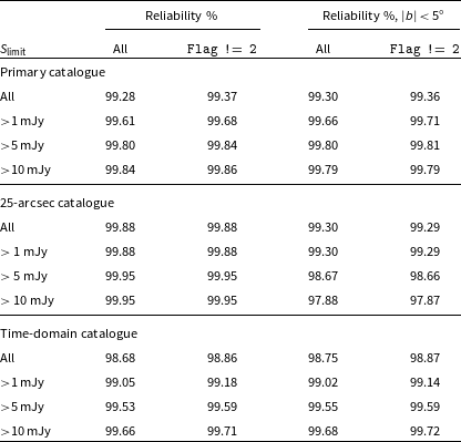
We summarise the source counts (and normalised source counts with and without completeness corrections) in Table 3. The normalised source counts are also shown in Fig. 12 for the RACS-mid catalogues, scaled to 1.4 GHz assuming $\alpha=-0.8$
alongside similar source counts from a range of other surveys, including RACS-low, FIRST (reported by White et al. Reference White, Becker, Helfand and Gregg1997), the compilation of 1.4-GHz source counts by Zotti et al. (2010, see references therein), and source counts from the DEEP2 catalogue (Matthews et al. Reference Matthews, Condon, Cotton and Mauch2021). We also show the ‘corrected’ RACS-mid source counts, after accounting for the flux density recovery fraction from Fig. 11(iv) and 11(v). After applying corrections for incompleteness, we find generally good agreement with existing source counts, with some deviation at low and high flux densities.
$\alpha=-0.8$
alongside similar source counts from a range of other surveys, including RACS-low, FIRST (reported by White et al. Reference White, Becker, Helfand and Gregg1997), the compilation of 1.4-GHz source counts by Zotti et al. (2010, see references therein), and source counts from the DEEP2 catalogue (Matthews et al. Reference Matthews, Condon, Cotton and Mauch2021). We also show the ‘corrected’ RACS-mid source counts, after accounting for the flux density recovery fraction from Fig. 11(iv) and 11(v). After applying corrections for incompleteness, we find generally good agreement with existing source counts, with some deviation at low and high flux densities.
At low flux densities ( $<$
2 mJy), the source counts from the primary catalogue follow the low-flux density bins from the Zotti et al. (Reference de Zotti, Massardi, Negrello and Wall2010) compilation and the DEEP2 source counts from Matthews et al. (Reference Matthews, Condon, Cotton and Mauch2021) until flux density bins reach
$<$
2 mJy), the source counts from the primary catalogue follow the low-flux density bins from the Zotti et al. (Reference de Zotti, Massardi, Negrello and Wall2010) compilation and the DEEP2 source counts from Matthews et al. (Reference Matthews, Condon, Cotton and Mauch2021) until flux density bins reach $\sim$ $0.6$
mJy. This mirrors what is seen with the RACS-low catalogue. Conversely, the 25-arcsec RACS-mid catalogue shows a decrease in the corrected source counts at
$0.6$
mJy. This mirrors what is seen with the RACS-low catalogue. Conversely, the 25-arcsec RACS-mid catalogue shows a decrease in the corrected source counts at $\sim$
1 mJy, though this is at the detection limit of the survey. In the high-flux density bins, the primary catalogue fails to report some of the brighter sources in the sky. Some of the brightest extended sources such as Fornax A are not recovered well in the data as described in Section 3.5 in Reference DuchesnePaper IV and may be split into smaller sources during source-finding. Such bright sources are therefore under-represented in the RACS-mid catalogues. We do not correct these high flux density bins for incompleteness as this requires a complex visibility-based process rather than our image-based sky model injection described in Section 4.6 and is beyond the scope of this brief source count assessment.
$\sim$
1 mJy, though this is at the detection limit of the survey. In the high-flux density bins, the primary catalogue fails to report some of the brighter sources in the sky. Some of the brightest extended sources such as Fornax A are not recovered well in the data as described in Section 3.5 in Reference DuchesnePaper IV and may be split into smaller sources during source-finding. Such bright sources are therefore under-represented in the RACS-mid catalogues. We do not correct these high flux density bins for incompleteness as this requires a complex visibility-based process rather than our image-based sky model injection described in Section 4.6 and is beyond the scope of this brief source count assessment.
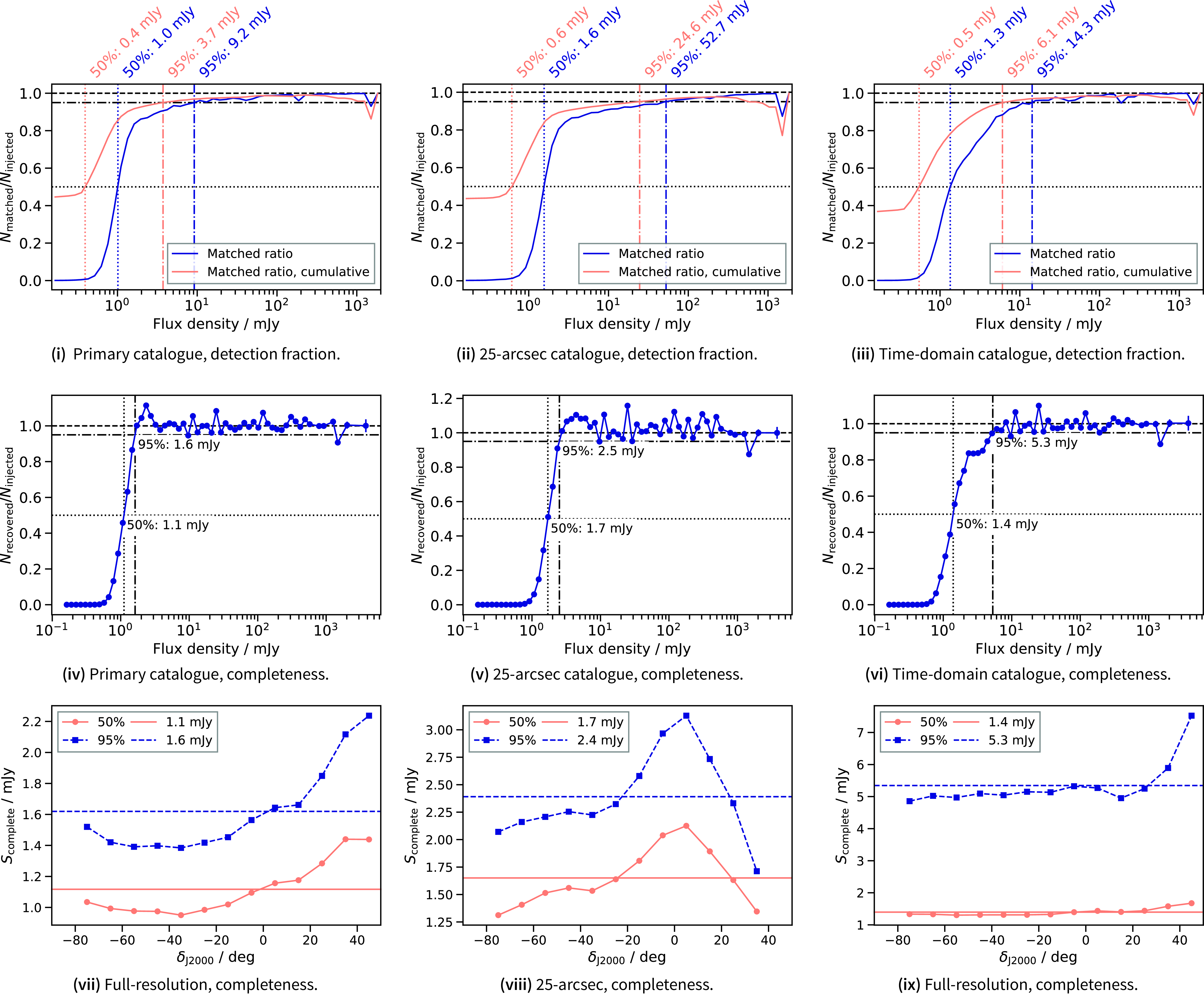
Figure 11. Assessment of the completeness of the three RACS-mid catalogues. (i)–(iii): The fraction of detected model sources matched to the input SKA sky model. The red lines correspond to matched fraction in flux density bins, while the blue line corresponds to the integrated matched fraction. 50% and 95% matched fractions are indicated on the plots. (iv)–(vi): An estimate of completeness as the fraction of flux density recovered in the model images as a function of flux density. 50% and 95% completeness fractions are shown on the plots. (vii)–(ix): An estimate of the 50% and 95% completeness ( $S_{\text{complete}}$
) as a function of declination, with the mean completeness shown as horizontal lines.
$S_{\text{complete}}$
) as a function of declination, with the mean completeness shown as horizontal lines.
4.8. Matching to external catalogues
For the following sections, we investigate the brightness scale and astrometry of the primary catalogue and the 25-arcsec catalogue. Due to similarities with the source lists used for validation in Reference DuchesnePaper IV, some comparisons with the time-domain catalogue are not repeated. We expect similarities with the primary catalogue and the 25-arcsec catalogue, though due to the additional mosaicking and image-based convolution it is worth confirming we have not introduced any significant systematic effects into the data.
For direct comparisons of flux density measurements and astrometry we look to the NVSS (Condon et al. Reference Condon, Cotton, Greisen, Yin, Perley, Taylor and Broderick1998) at 1.4 GHz, FIRST (Becker et al. Reference Becker, White and Helfand1995; White et al. Reference White, Becker, Helfand and Gregg1997; Helfand et al. Reference Helfand, White and Becker2015), and the 42-deg $^{2}$
region of the WALLABY pre-pilot catalogue (Grundy et al. Reference Grundy2023). FIRST is catalogued at both the same frequency as NVSS (for data prior to 2011) and at 1 335 MHz (for data from 2011). FIRST sources detected in data from 2011 onward comprise
$^{2}$
region of the WALLABY pre-pilot catalogue (Grundy et al. Reference Grundy2023). FIRST is catalogued at both the same frequency as NVSS (for data prior to 2011) and at 1 335 MHz (for data from 2011). FIRST sources detected in data from 2011 onward comprise $\sim$
6% of the full FIRST catalogue but are exclusively in the region that overlaps with RACS-mid. To account for this in the FIRST data, we scale the flux density measurements, S, of the 2011-onward data to match the 1 400-MHz data assuming a power law of the form
$\sim$
6% of the full FIRST catalogue but are exclusively in the region that overlaps with RACS-mid. To account for this in the FIRST data, we scale the flux density measurements, S, of the 2011-onward data to match the 1 400-MHz data assuming a power law of the form $S \propto \nu^{\alpha}$
with
$S \propto \nu^{\alpha}$
with $\alpha = -0.8$
. For comparison to catalogues at other frequencies, we use the RACS-low catalogue (Reference HalePaper II), SUMSS (Bock et al. Reference Bock, Large and Sadler1999; Mauch et al. Reference Mauch, Murphy, Buttery, Curran, Hunstead, Piestrzynski, Robertson and Sadler2003), the TIFRFootnote 11 GMRTFootnote 12 Sky Survey alternate data release 1 (TGSS; Intema et al. Reference Intema, Jagannathan, Mooley and Frail2017) and the LOFARFootnote 13 Two-metre Sky Survey data release 2 (LoTSS-DR2; Shimwell et al. Reference Shimwell2022) catalogue. These catalogues provide a range of comparisons in the frequency range 144–1 400 MHz. For additional astrometry assessment, we also compare to the VLA Sky Survey (VLASS; Lacy et al. Reference Lacy2020) first epoch ‘quick-look’ catalogue (hereinafter VLASS-QL; Gordon et al. Reference Gordon2021).
$\alpha = -0.8$
. For comparison to catalogues at other frequencies, we use the RACS-low catalogue (Reference HalePaper II), SUMSS (Bock et al. Reference Bock, Large and Sadler1999; Mauch et al. Reference Mauch, Murphy, Buttery, Curran, Hunstead, Piestrzynski, Robertson and Sadler2003), the TIFRFootnote 11 GMRTFootnote 12 Sky Survey alternate data release 1 (TGSS; Intema et al. Reference Intema, Jagannathan, Mooley and Frail2017) and the LOFARFootnote 13 Two-metre Sky Survey data release 2 (LoTSS-DR2; Shimwell et al. Reference Shimwell2022) catalogue. These catalogues provide a range of comparisons in the frequency range 144–1 400 MHz. For additional astrometry assessment, we also compare to the VLA Sky Survey (VLASS; Lacy et al. Reference Lacy2020) first epoch ‘quick-look’ catalogue (hereinafter VLASS-QL; Gordon et al. Reference Gordon2021).
For the remainder of the validation work, unless otherwise specified, we are only considering unresolved (Flag = 0) sources in the RACS-mid catalogues. For the comparison catalogues, we generally only look at unresolved sources if the survey angular resolution is on average higher than RACS-mid. In the case of RACS-low and the WALLABY pre-pilot catalogue, we use the same unresolved criteria described in Reference HalePaper II and Grundy et al. (Reference Grundy2023) (39.6% and 76.5% unresolved, respectively), but for the remaining comparison catalogues we employ the simpler criteria. For the FIRST, VLASS-QL, and LoTSS-DR2 catalogues we take sources that satisfy $|\log_{10}(S_{\text{int}}/S_{\text{peak}})| < \log_{10}(1.2)$
as unresolved. In the case of LoTSS-DR2, because of significantly blurring point sources show ratios closer to
$|\log_{10}(S_{\text{int}}/S_{\text{peak}})| < \log_{10}(1.2)$
as unresolved. In the case of LoTSS-DR2, because of significantly blurring point sources show ratios closer to $\sim$ $1.25$
, and for that catalogue we shift the ratio criterion by an additional
$1.25$
, and for that catalogue we shift the ratio criterion by an additional $\log_{10}(0.25)$
. With this criterion we find unresolved fractions for the FIRST, VLASS-QL, and LoTSS-DR2 of 44.9, 26.1, and 47.6%. We note for LoTSS-DR2 Shimwell et al. (Reference Shimwell2022) find a resolved fraction of 8.0%. In this case we are more concerned with confidence in determining unresolved sources so we remove potentially resolved sources, whereas Shimwell et al. (Reference Shimwell2022) were focused on resolved sources and conversely remove potentially unresolved sources with their method.
$\log_{10}(0.25)$
. With this criterion we find unresolved fractions for the FIRST, VLASS-QL, and LoTSS-DR2 of 44.9, 26.1, and 47.6%. We note for LoTSS-DR2 Shimwell et al. (Reference Shimwell2022) find a resolved fraction of 8.0%. In this case we are more concerned with confidence in determining unresolved sources so we remove potentially resolved sources, whereas Shimwell et al. (Reference Shimwell2022) were focused on resolved sources and conversely remove potentially unresolved sources with their method.
Finally, when cross-matchingFootnote 14 the catalogues we consider only isolated sources in the respective catalogues. Isolated sources in this case are defined as those with no neighbours within $2\theta_{\text{major}}$
for the given catalogue. Cross-matching is then done with a match radius equal to half the PSF major FWHM for the survey with the lowest angular resolution. After cross-matching with these strict criteria we find that the 25-arcsec catalogue results in the largest number of matches in catalogues with angular resolutions
$2\theta_{\text{major}}$
for the given catalogue. Cross-matching is then done with a match radius equal to half the PSF major FWHM for the survey with the lowest angular resolution. After cross-matching with these strict criteria we find that the 25-arcsec catalogue results in the largest number of matches in catalogues with angular resolutions $\gtrsim 25 \times 25$
arcsec
$\gtrsim 25 \times 25$
arcsec $^{2}$
. The time-domain catalogue results in the least matches simply because the duplication of sources makes the isolation criterion difficult to satisfy, and generally there will be few cross-matches in the overlap regions between tiles. For assessment of the overlap regions, we refer the reader to Reference DuchesnePaper IV or Section 4.12.
$^{2}$
. The time-domain catalogue results in the least matches simply because the duplication of sources makes the isolation criterion difficult to satisfy, and generally there will be few cross-matches in the overlap regions between tiles. For assessment of the overlap regions, we refer the reader to Reference DuchesnePaper IV or Section 4.12.
Table 3. Tabulated source counts for the primary and 25-arcsec RACS-mid catalogues.
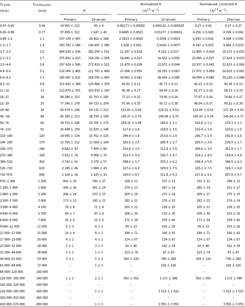
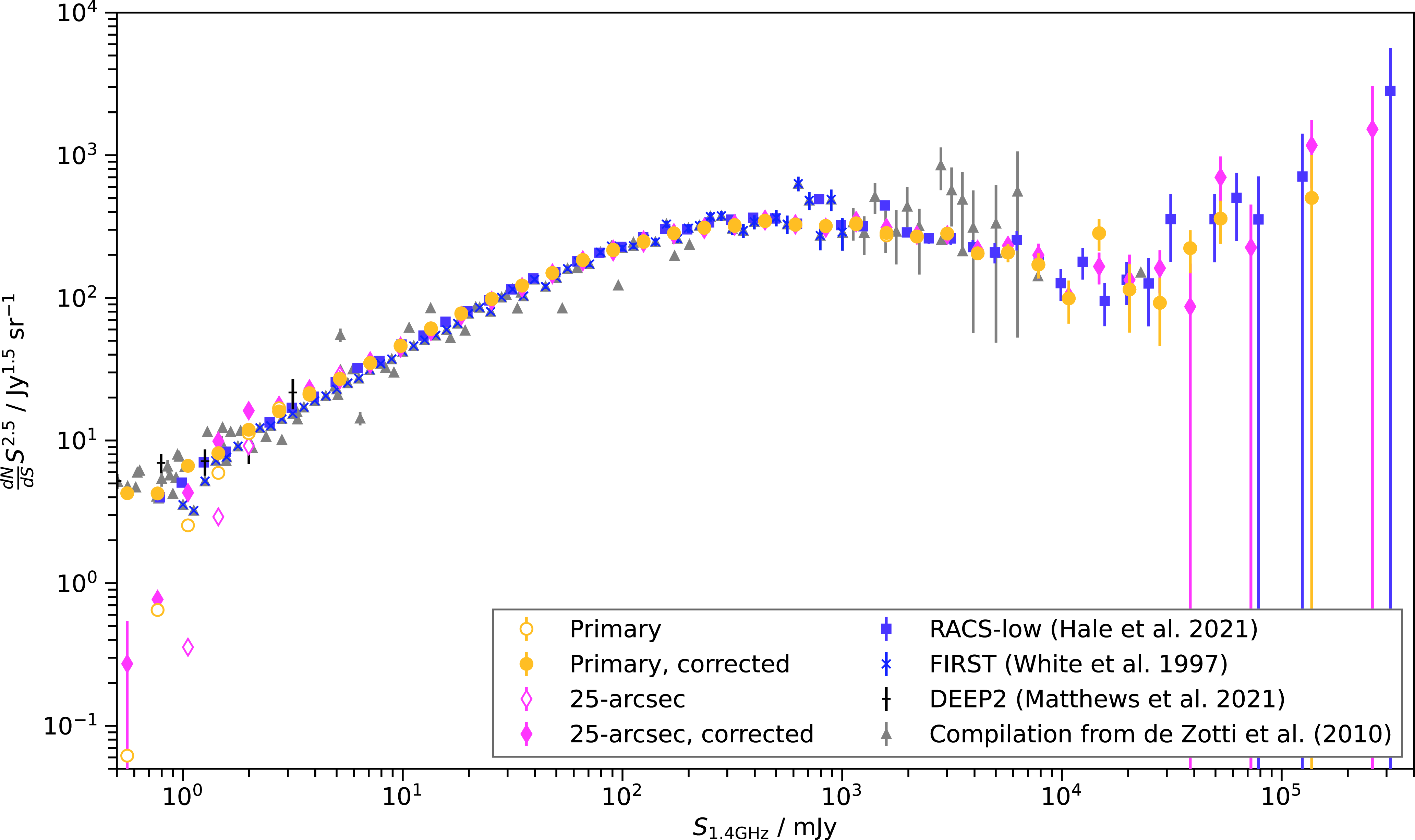
Figure 12. The corrected and uncorrected source counts from the primary and 25-arcsec RACS-mid catalogues (excluding $|b|<5^{\circ}$
). Source counts from a selection of other surveys are shown for reference, including the 1.4-GHz compilation from de Zotti et al. (Reference de Zotti, Massardi, Negrello and Wall2010), the 1997 FIRST catalogue White et al. (Reference White, Becker, Helfand and Gregg1997), Matthews et al. (Reference Matthews, Condon, Cotton and Mauch2021), and RACS-low (Reference HalePaper II).
$|b|<5^{\circ}$
). Source counts from a selection of other surveys are shown for reference, including the 1.4-GHz compilation from de Zotti et al. (Reference de Zotti, Massardi, Negrello and Wall2010), the 1997 FIRST catalogue White et al. (Reference White, Becker, Helfand and Gregg1997), Matthews et al. (Reference Matthews, Condon, Cotton and Mauch2021), and RACS-low (Reference HalePaper II).
The numbers of sources cross-matched for each RACS-mid catalogue and external catalogue are reported in Table 4.
Table 4. Median reported properties of sources cross-matched between the RACS-mid catalogues and other surveys, with and without flux density limits applied.

a Frequency of the comparison survey.
b
Sources detected in data from 2011 are scaled from 1 335 MHz assuming a power law with spectral index $-0.7$
.
$-0.7$
.
4.9. Photometry
As part of the RACS-mid processing, we used cross-matches to NVSS and SUMSS to correct for time-dependent brightness scale variations (see Section 2.6 in Reference DuchesnePaper IV and further discussion of this issue in Section 3.3.3 in Reference McConnellPaper I). By construction, this ensures the bulk brightness scale between RACS-mid and the NVSS and SUMSS is consistent within the assumed spectral index of $-0.82$
.Footnote 15 Despite this it is still worth comparing the catalogues produced here due to a difference in the images and source-finding.
$-0.82$
.Footnote 15 Despite this it is still worth comparing the catalogues produced here due to a difference in the images and source-finding.
4.9.1. External brightness scale
For a direct brightness scale comparison, Fig. 13 shows the ratio of integrated flux densities of sources cross-matched between NVSS, FIRST, and the WALLABY pre-pilot catalogue for the three RACS-mid catalogues independently as a function of the RACS-mid flux density. Sources in Fig. 13 are coloured by $S_{\text{int}}/S_{\text{peak}}$
as measured in the respective RACS-mid catalogues. Generally
$S_{\text{int}}/S_{\text{peak}}$
as measured in the respective RACS-mid catalogues. Generally $S_{\text{int}}/S_{\text{peak}}$
has a restricted range as these are intended to be unresolved sources as defined in Section 4.4. Fig. 13 also displays a histogram of the distribution of the flux density ratios.
$S_{\text{int}}/S_{\text{peak}}$
has a restricted range as these are intended to be unresolved sources as defined in Section 4.4. Fig. 13 also displays a histogram of the distribution of the flux density ratios.
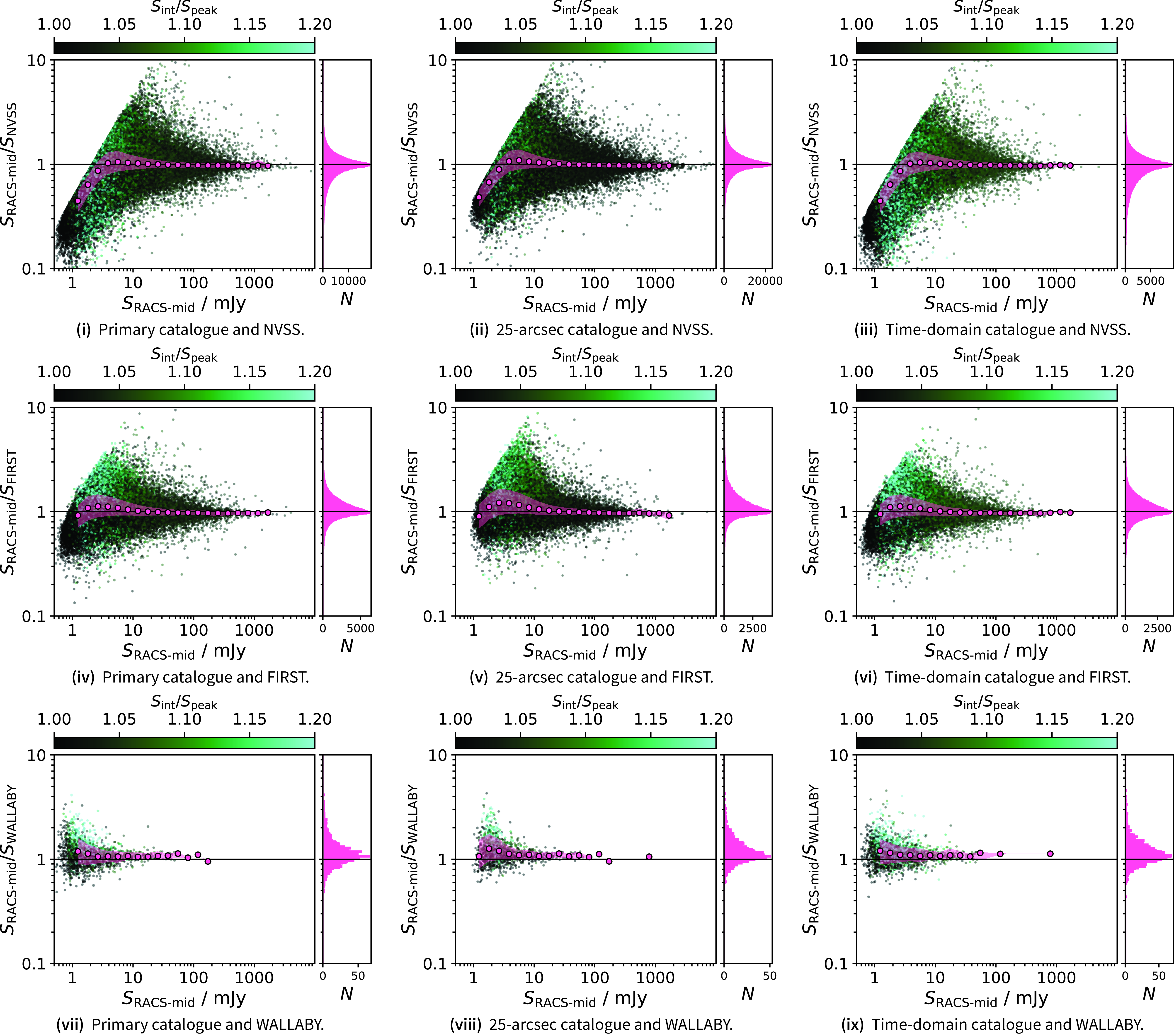
Figure 13. Flux density ratio of unresolved sources cross-matched in the RACS-mid catalogues and the NVSS (top panels), FIRST (centre panels), and the WALLABY pre-pilot catalogue (bottom panels) as a function of the RACS-mid flux density measurements. Background data points are coloured by their SNR in the RACS-mid data. The solid, black line in each panel indicates a ratio of 1. Pink points indicate median flux density ratios in bins, with the shaded pink region covering the $16\text{th}$
and
$16\text{th}$
and $84\text{th}$
percentiles in each bin.
$84\text{th}$
percentiles in each bin.
The results for the three RACS-mid catalogues are generally similar, and we report in Table 4 the median flux density ratios for each cross-match alongside the median flux density ratio after applying a 10 mJy limit to the RACS-mid catalogue. For all three RACS-mid catalogues, the 10-mJy limit provides median ratios of $\sim$ $0.99$
–
$0.99$
– $1.00$
for the NVSS and FIRST cross-matches broadly consistent with Reference DuchesnePaper IV. The RACS-mid data shows marginally higher flux densities (
$1.00$
for the NVSS and FIRST cross-matches broadly consistent with Reference DuchesnePaper IV. The RACS-mid data shows marginally higher flux densities ( $\sim$
10%) than the WALLABY pre-pilot data, though the WALLABY pre-pilot data is already found to be underluminous with respect to the NVSS with additional positional-dependent variation (For et al. Reference For2021; Grundy et al. Reference Grundy2023). The full sample shows more variation, with the low-brightness flux density ratios showing systematic deviation, different for the low-resolution NVSS and high-resolution FIRST and WALLABY pre-pilot data. In the case of the NVSS, the low-brightness cross-matches tend towards
$\sim$
10%) than the WALLABY pre-pilot data, though the WALLABY pre-pilot data is already found to be underluminous with respect to the NVSS with additional positional-dependent variation (For et al. Reference For2021; Grundy et al. Reference Grundy2023). The full sample shows more variation, with the low-brightness flux density ratios showing systematic deviation, different for the low-resolution NVSS and high-resolution FIRST and WALLABY pre-pilot data. In the case of the NVSS, the low-brightness cross-matches tend towards $<$
1, which is a result of faint sources in the NVSS catalogue being pushed above the detection threshold due to scatter in the flux densities (i.e. Eddington bias). Conversely, the low-brightness end of the FIRST and WALLABY pre-pilot cross-matches shows a bump
$<$
1, which is a result of faint sources in the NVSS catalogue being pushed above the detection threshold due to scatter in the flux densities (i.e. Eddington bias). Conversely, the low-brightness end of the FIRST and WALLABY pre-pilot cross-matches shows a bump $>$
1 in the ratios before also dropping
$>$
1 in the ratios before also dropping $<$
1. The increase in flux density as measured in RACS-mid can be explained by an increase in truly extended sources being cross-matched, which are not as well-detected in FIRST. This indicates our criteria for ‘unresolved’ sources defined in Section 4.4 has overestimated the true unresolved fraction for sources
$<$
1. The increase in flux density as measured in RACS-mid can be explained by an increase in truly extended sources being cross-matched, which are not as well-detected in FIRST. This indicates our criteria for ‘unresolved’ sources defined in Section 4.4 has overestimated the true unresolved fraction for sources $<$
10 mJy.
$<$
10 mJy.
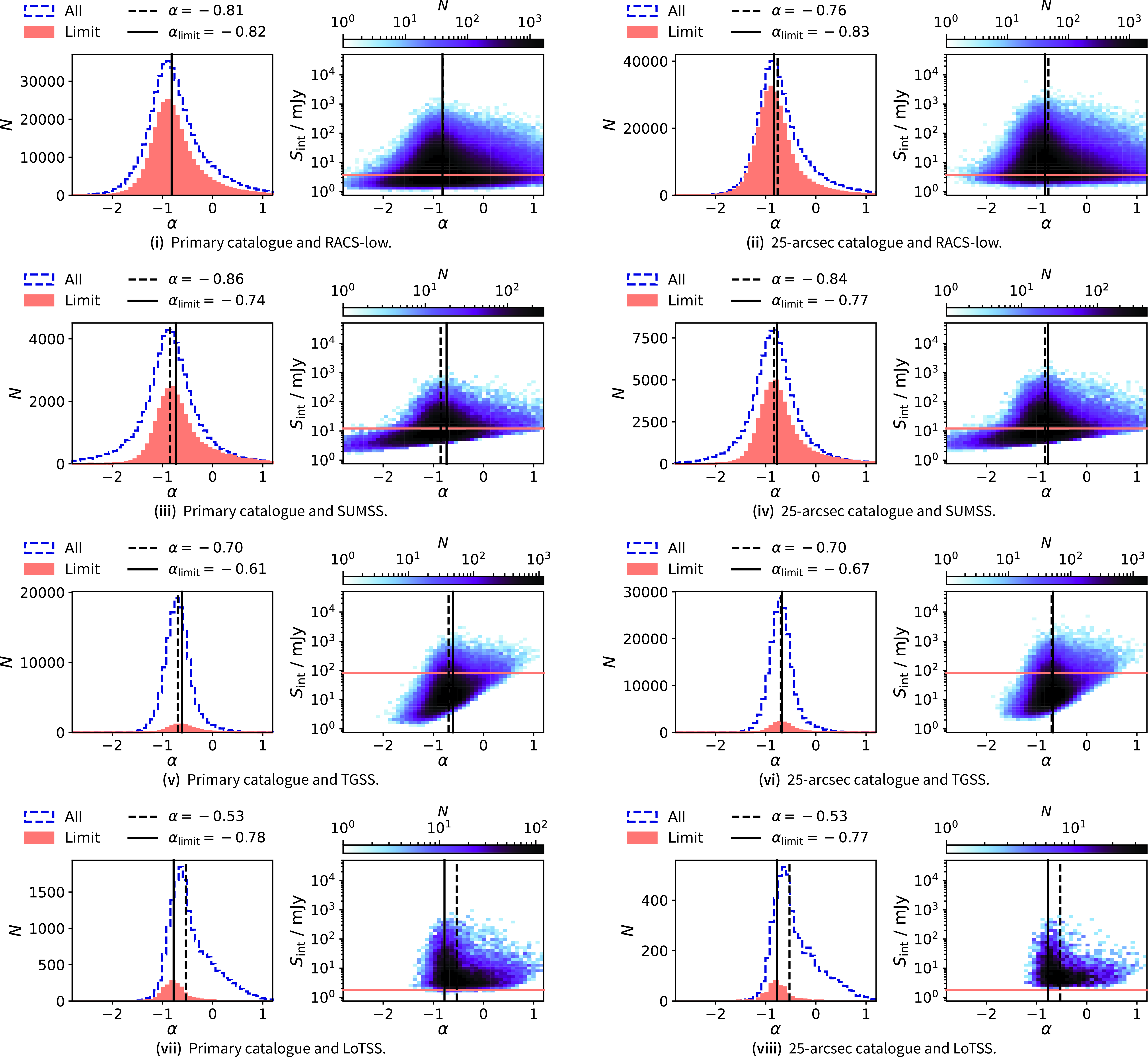
Figure 14. Spectral indices of sources cross-matched between the RACS-mid and RACS-low (i)–(ii), SUMSS (iii)–(iv), TGSS-ADR1 (v)–(vi), and LoTSS-DR2 (vii)–(viii) for both the primary catalogue (left) and the 25-arcsec catalogue (right). Left panels. Histogram of $\alpha$
with all sources (blue, dashed) and with flux density limits (orange, filled). Median
$\alpha$
with all sources (blue, dashed) and with flux density limits (orange, filled). Median $\alpha$
values are also shown. Right panels. 2D histogram of RACS-mid flux density measurements against spectral index. The red line shows the RACS-mid flux density limit for the given catalogue comparison.
$\alpha$
values are also shown. Right panels. 2D histogram of RACS-mid flux density measurements against spectral index. The red line shows the RACS-mid flux density limit for the given catalogue comparison.
4.9.2. Spectral indices
For comparisons with surveys at significantly different frequencies, we follow Reference HalePaper II and opt to assess the spectral indices of sources cross-matched between the RACS-mid primary catalogue and 25-arcsec catalogue and other surveys. For this purpose, we use the RACS-low catalogue (Reference HalePaper II), the SUMSS catalogue (Mauch et al. Reference Mauch, Murphy, Buttery, Curran, Hunstead, Piestrzynski, Robertson and Sadler2003), the TGSS ADR1 (Intema et al. Reference Intema, Jagannathan, Mooley and Frail2017), and the LoTSS-DR2 catalogue (Shimwell et al. Reference Shimwell2022). A two-point spectral index, $\alpha$
, is calculated for cross-matched sources assuming a power law, following
$\alpha$
, is calculated for cross-matched sources assuming a power law, following
 \begin{equation}\alpha = \frac{\log_{\text{10}}\left(S_{\text{RACS-mid}} / S_{\text{survey}}\right)}{\log_{\text{10}}\left(1\,367.5 / \nu_{\text{survey}}\right)} \,, \end{equation}
where $S_{\text{RACS-mid}}$
and
$S_{\text{RACS-mid}}$
and $S_{\text{survey}}$
are the integrated flux densities of the given source in the RACS-mid catalogue and comparison survey, respectively, and
$S_{\text{survey}}$
are the integrated flux densities of the given source in the RACS-mid catalogue and comparison survey, respectively, and $\nu_{\text{survey}}$
is the survey frequency.
$\nu_{\text{survey}}$
is the survey frequency.
Following Reference HalePaper II we also create a subsample by applying a flux density limit to each survey to remove some sensitivity bias—this helps reduce artificial flattening or steepening of the median spectra. We assume limits in the range $\alpha = -0.8\pm1.2$
and set a flux density limit for both the RACS-mid catalogues and comparison catalogues to be either side of that range, depending on which survey is higher in frequency. The resultant limits are reported in Table 4. Table 4 also reports the median spectral indices for the full sample and flux-limited samples for each RACS-mid catalogue and comparison survey. We also plot the histogram of spectral indices (with and without the flux density limit) in Fig. 14 alongside a 2D histogram showing RACS-mid flux density as a function of spectral index. The flux-limited subsample is included in the histograms to highlight the reduced number of sources, and the RACS-mid flux density limit is also shown in 2D histogram for reference (though note the comparison survey limit is not shown). Where relevant the spectral indices of sources matched between catalogues are generally consistent with results from Reference DuchesnePaper IV.
$\alpha = -0.8\pm1.2$
and set a flux density limit for both the RACS-mid catalogues and comparison catalogues to be either side of that range, depending on which survey is higher in frequency. The resultant limits are reported in Table 4. Table 4 also reports the median spectral indices for the full sample and flux-limited samples for each RACS-mid catalogue and comparison survey. We also plot the histogram of spectral indices (with and without the flux density limit) in Fig. 14 alongside a 2D histogram showing RACS-mid flux density as a function of spectral index. The flux-limited subsample is included in the histograms to highlight the reduced number of sources, and the RACS-mid flux density limit is also shown in 2D histogram for reference (though note the comparison survey limit is not shown). Where relevant the spectral indices of sources matched between catalogues are generally consistent with results from Reference DuchesnePaper IV.
4.10. Astrometry
As noted in Reference DuchesnePaper IV, there are two astrometric errors that exist in the RACS-mid data (see Figures 36 and 38 in Reference DuchesnePaper IV). Firstly, the self-calibration process, performed independently for each PAF beam image prior to mosaicking, introduces up to pixel-scale offsets in both right ascension (R. A.) and declination. This effect is not dependent on the SNR of the sources in the field. The result of this effect is an uncertainty in the astrometric accuracy up to $\pm 1$
–2 arcsec. The second effect is a systematic declination-dependent offset in declination which is currently undiagnosed. This effect results in up to
$\pm 1$
–2 arcsec. The second effect is a systematic declination-dependent offset in declination which is currently undiagnosed. This effect results in up to $\sim$
2 arcsec offset at the highest declination of the survey. While we cannot reasonably correct the beam-to-beam astrometric precision at this stage, we do attempt to remove the systematic declination-dependent offets.
$\sim$
2 arcsec offset at the highest declination of the survey. While we cannot reasonably correct the beam-to-beam astrometric precision at this stage, we do attempt to remove the systematic declination-dependent offets.
For removal of the declination-dependent declination offset, we cross-match the unresolved time-domain RACS-mid catalogue to sources in the third realisation of the International Celestial Reference Frame (ICRF3; Charlot et al. Reference Charlot2020). The time-domain catalogue is used for this purpose to take advantage of sources in the overlap regions. Since the ICRF3 catalogue is sparse compared to RACS-mid, we do not use the isolated source restriction. We define the declination offsets as
 \begin{equation}\Delta\delta = (\delta_{\text{RACS-mid}} - \delta_{\text{ICRF3}}) \quad \text{arcsec}, \end{equation}
and fit a range of generic polynomials covering $0\text{th}$
to
$0\text{th}$
to $4\text{th}$
orders. We use the SNR of the RACS-mid flux density measurement to weight the fitting procedure, and use the Akaike Information Criterion (AIC; Akaike Reference Akaike1974) as a means to select the appropriate order polynomial. As initial polynomial fitting only considers measurement uncertainties in
$4\text{th}$
orders. We use the SNR of the RACS-mid flux density measurement to weight the fitting procedure, and use the Akaike Information Criterion (AIC; Akaike Reference Akaike1974) as a means to select the appropriate order polynomial. As initial polynomial fitting only considers measurement uncertainties in $\delta_{\text{J2000}}$
reported by PyBDSF, we estimate uncertainties on the polynomial fit by repeating the fitting procedure after adding Gaussian noise to the model offsets. The added noise is drawn from a Gaussian distribution, assuming the mean and standard deviation of
$\delta_{\text{J2000}}$
reported by PyBDSF, we estimate uncertainties on the polynomial fit by repeating the fitting procedure after adding Gaussian noise to the model offsets. The added noise is drawn from a Gaussian distribution, assuming the mean and standard deviation of $\Delta\delta$
(
$\Delta\delta$
( $-0.26$
and
$-0.26$
and $1.16$
arcsec, respectively). With this, we find a
$1.16$
arcsec, respectively). With this, we find a $2\text{nd}$
-order polynomial of the form
$2\text{nd}$
-order polynomial of the form
 \begin{equation} \Delta\delta = 0.175(34) - 0.0150(9)\delta - 0.000301(18) \delta^2 \quad \text{arcsec}, \end{equation}
where $\delta={\delta_{\text{J2000}}}^{\circ}$
and is the declination of the source in the RACS-mid catalogue.
$\delta={\delta_{\text{J2000}}}^{\circ}$
and is the declination of the source in the RACS-mid catalogue.
Fig. 15(i)–15(iii) shows the RACS-mid—ICRF3 declination offsets as a function of declination in the top panels, with medians in declination bins shown as blue circles. The upper panels highlight both the lower astrometric precision at high declination (above $\delta_{\text{J2000}} \approx 20^{\circ}$
) and the general trend towards negative offsets at high and low declination. We show on the upper panels the selected
$\delta_{\text{J2000}} \approx 20^{\circ}$
) and the general trend towards negative offsets at high and low declination. We show on the upper panels the selected $2\text{nd}$
-order polynomial, derived from the time-domain catalogue, and the lower panels show the same data but with removal of the offset model (i.e. the ‘corrected’ declination). We report the median
$2\text{nd}$
-order polynomial, derived from the time-domain catalogue, and the lower panels show the same data but with removal of the offset model (i.e. the ‘corrected’ declination). We report the median $\Delta\alpha$
and
$\Delta\alpha$
and $\Delta\delta$
against the ICRF3 in Table 5 along with
$\Delta\delta$
against the ICRF3 in Table 5 along with $1\sigma$
uncertainties. These remain similar to results from Reference DuchesnePaper IV. We also report the median declination offset after applying the model correction—this results in no substantial difference to the overall median and uncertainty.
$1\sigma$
uncertainties. These remain similar to results from Reference DuchesnePaper IV. We also report the median declination offset after applying the model correction—this results in no substantial difference to the overall median and uncertainty.
Table 5 also reports similar median offsets for comparisons with a range of other surveys, both with and without the declination correction. Notably, the declination correction does not make a large difference in most cases as the correction is close to the level of the uncertainty (largely driven by the aforementioned beam-to-beam variation). The exception to this is for the comparison to LoTSS-DR2. For LoTSS-DR2, sky coverage begins at $\delta_{\text{J2000}}>15^{\circ}$
so suffers from the most extreme declination offsets. A column containing the ‘corrected’ declination is added to all RACS-mid catalogues, though we retain the original declination column as well. Users may find cross-matching to high-declination regions more straightforward with the corrected declination measurements.
$\delta_{\text{J2000}}>15^{\circ}$
so suffers from the most extreme declination offsets. A column containing the ‘corrected’ declination is added to all RACS-mid catalogues, though we retain the original declination column as well. Users may find cross-matching to high-declination regions more straightforward with the corrected declination measurements.
In Fig. 16 we show coordinate offsets for the primary and 25-arcsec catalogues against the ICRF3, RACS-low, VLASS-QL, and LoTSS-DR2 as a function of source SNR in the RACS-mid catalogues. In Fig. 16 we also show binned median offsets as a function of SNR, with $1\sigma$
error ranges shown as shaded regions. Note that the uncertainty remains fairly constant as a function of SNR, as mentioned in Reference DuchesnePaper IV as the beam-to-beam astrometric offset introduced by self-calibration are direction- and source-independent. The lower panels of Fig. 16 show the declination offsets after the correction described in Equation (9).
$1\sigma$
error ranges shown as shaded regions. Note that the uncertainty remains fairly constant as a function of SNR, as mentioned in Reference DuchesnePaper IV as the beam-to-beam astrometric offset introduced by self-calibration are direction- and source-independent. The lower panels of Fig. 16 show the declination offsets after the correction described in Equation (9).

Figure 15. Declination ( $\Delta\delta$
) offsets from the ICRF3 as a function of declination for the primary catalogue (i) the auxiliary 25-arcsec catalogue (ii), and the auxiliary time-domain catalogue (iii). The fitted declination-dependent polynomial, derived from the auxiliary time-domain catalogue for all catalogues, is shown on the upper panels, and the lower panels show the residual offsets after subtraction of the derived model.
$\Delta\delta$
) offsets from the ICRF3 as a function of declination for the primary catalogue (i) the auxiliary 25-arcsec catalogue (ii), and the auxiliary time-domain catalogue (iii). The fitted declination-dependent polynomial, derived from the auxiliary time-domain catalogue for all catalogues, is shown on the upper panels, and the lower panels show the residual offsets after subtraction of the derived model.
The overall median offsets for each catalogue comparison are also reported in Table 5. Generally absolute median offsets are $\lesssim$ $0.3$
arcsec with the except of the aforementioned declination offset in LoTSS-DR2 and right ascension offsets with RACS-low (
$0.3$
arcsec with the except of the aforementioned declination offset in LoTSS-DR2 and right ascension offsets with RACS-low ( $\sim +0.4$
arcsec) and SUMSS (
$\sim +0.4$
arcsec) and SUMSS ( $\sim +0.6$
arcsec). A right ascension offset for RACS-low was reported by Reference HalePaper II and is intrinsic to that catalogue. It is likely this is an elevation-dependent offset (the true form of the declination-dependent trend we see here) and with RACS-low being observed off the meridian the offset manifests in both declination and right ascension.
$\sim +0.6$
arcsec). A right ascension offset for RACS-low was reported by Reference HalePaper II and is intrinsic to that catalogue. It is likely this is an elevation-dependent offset (the true form of the declination-dependent trend we see here) and with RACS-low being observed off the meridian the offset manifests in both declination and right ascension.
Table 5. Astrometric offsets of sources cross-matched between RACS-mid and external catalogues, with offsets defined as $\Delta\delta = \delta_{\text{RACS-mid}}-\delta_{\text{survey}}$
and
$\Delta\delta = \delta_{\text{RACS-mid}}-\delta_{\text{survey}}$
and $\Delta\alpha\cos\delta = (\alpha_{\text{RACS-mid}} - \alpha_{\text{survey}})\cos\delta$
for declination and R. A. offsets, respectively.
$\Delta\alpha\cos\delta = (\alpha_{\text{RACS-mid}} - \alpha_{\text{survey}})\cos\delta$
for declination and R. A. offsets, respectively.
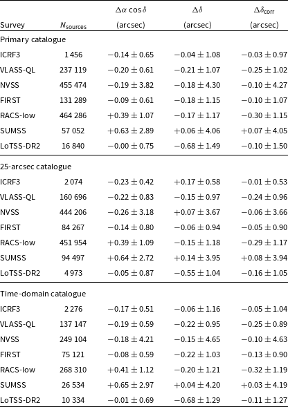
4.11. RACS-mid and other ASKAP surveys
4.11.1. RACS-low and RACS-mid at 25 arcsec
The goal of RACS is to create a global sky model for calibration and validation of the other ASKAP surveys and ASKAP observations in general. The global sky model is intended to be a combination of all three RACS bands from 887.5–1 632.5 MHz (low, mid, and high). While we are still awaiting RACS-high images and catalogues, we begin with an initial assessment of a sky model built between 887.5 and 1 367.5 MHz with the RACS-low and RACS-mid 25-arcsec catalogues. We perform simple cross-match between the source catalogues for each survey, taking sources that cross-match within $(\theta_{\text{major}}\theta_{\text{minor}})/4$
, where
$(\theta_{\text{major}}\theta_{\text{minor}})/4$
, where $\theta_{\text{major}}$
and
$\theta_{\text{major}}$
and $\theta_{\text{minor}}$
are the fitted major and minor axes. This variable match criterion is to account for extended sources, which may have different centres in each catalogue. More robust catalogue matching processes may be implemented in future combinations of RACS (e.g. the Positional Update and Matching Algorithm; Line et al. Reference Line, Webster, Pindor, Mitchell and Trott2017), taking into account expected spectral information. We scale the flux densities of the RACS-low catalogue to 1 367.5 MHz assuming the flux-limit median
$\theta_{\text{minor}}$
are the fitted major and minor axes. This variable match criterion is to account for extended sources, which may have different centres in each catalogue. More robust catalogue matching processes may be implemented in future combinations of RACS (e.g. the Positional Update and Matching Algorithm; Line et al. Reference Line, Webster, Pindor, Mitchell and Trott2017), taking into account expected spectral information. We scale the flux densities of the RACS-low catalogue to 1 367.5 MHz assuming the flux-limit median $\alpha=-0.83$
(see Section 4.9.2). For this cross-match, we are interested in the region that completely overlaps with both the RACS-low and RACS-mid 25-arcsec catalogues and we only consider sources within the declination range
$\alpha=-0.83$
(see Section 4.9.2). For this cross-match, we are interested in the region that completely overlaps with both the RACS-low and RACS-mid 25-arcsec catalogues and we only consider sources within the declination range $-80^{\circ}<\delta_{\text{J2000}}<+29^{\circ}$
, including the Galactic Plane. Note that the RACS-low catalogue is missing a small region below
$-80^{\circ}<\delta_{\text{J2000}}<+29^{\circ}$
, including the Galactic Plane. Note that the RACS-low catalogue is missing a small region below $\delta_{\text{J2000}}=+30^{\circ}$
and has patchy coverage below
$\delta_{\text{J2000}}=+30^{\circ}$
and has patchy coverage below $\delta_{\text{J2000}}=-80^{\circ}$
.
$\delta_{\text{J2000}}=-80^{\circ}$
.
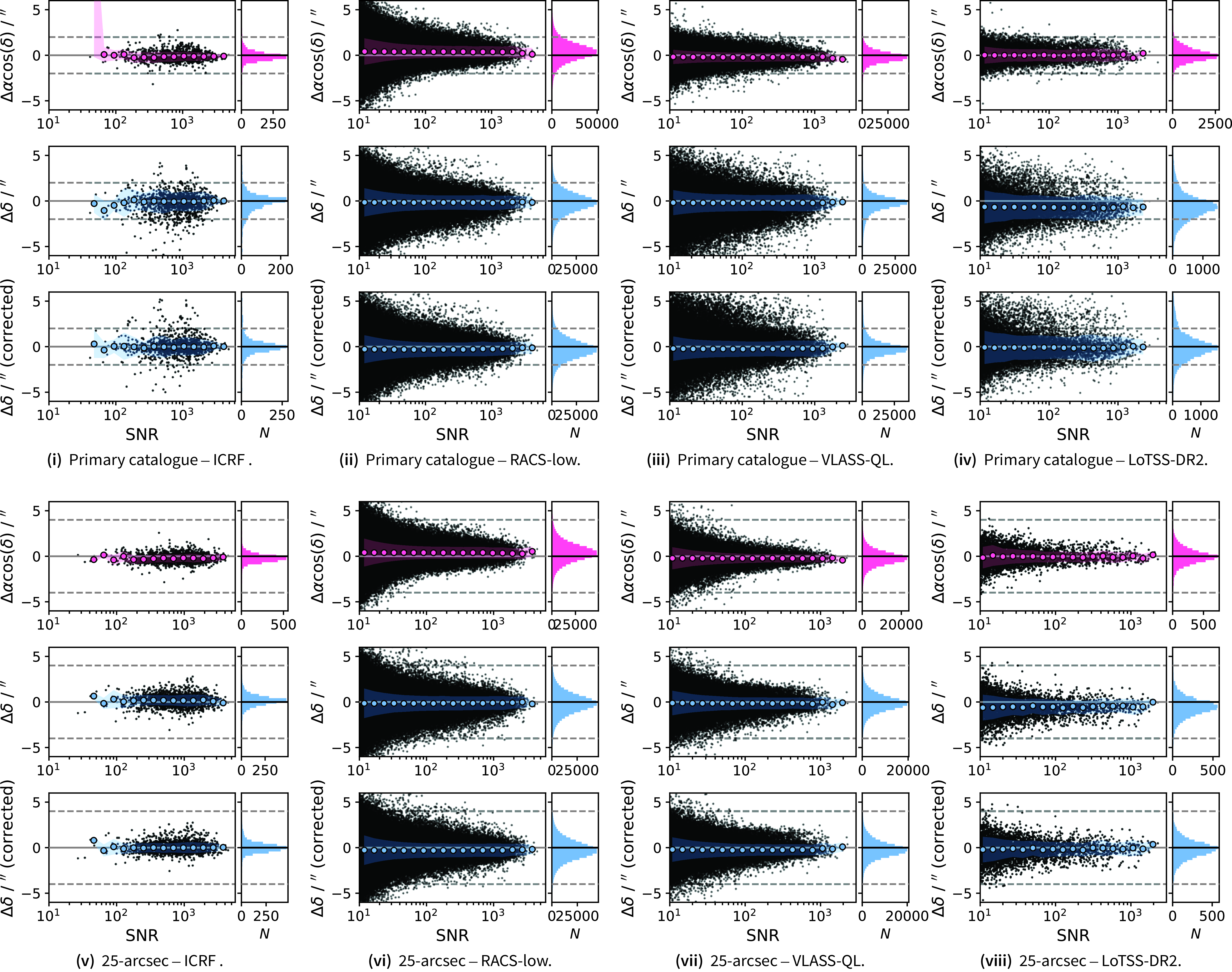
Figure 16. R. A. ( $\Delta\alpha\cos\left(\delta\right)$
) and declination (
$\Delta\alpha\cos\left(\delta\right)$
) and declination ( $\Delta\delta$
) offsets as a function of SNR for the primary catalogue [(i)–(iv)] and the 25-arcsec catalogue [(v)–(viii)]. Left. ICRF cross-match. Centre-left. RACS-low cross-match. Centre-right. VLASS-QL cross-match. Right. LoTSS-DR2 cross-match. In each panel, a dashed, grey line is drawn at
$\Delta\delta$
) offsets as a function of SNR for the primary catalogue [(i)–(iv)] and the 25-arcsec catalogue [(v)–(viii)]. Left. ICRF cross-match. Centre-left. RACS-low cross-match. Centre-right. VLASS-QL cross-match. Right. LoTSS-DR2 cross-match. In each panel, a dashed, grey line is drawn at $\pm2$
arcsec corresponding to the pixel size of the original RACS-mid images. Median values in SNR bins are also shown as coloured markers and the shaded regions indicate
$\pm2$
arcsec corresponding to the pixel size of the original RACS-mid images. Median values in SNR bins are also shown as coloured markers and the shaded regions indicate $\pm2\sigma$
for the SNR bins.
$\pm2\sigma$
for the SNR bins.
Fig. 17 shows the distribution of sources of both the RACS-mid and RACS-low 25-arcsec catalogues, as a function of flux density (scaled to 1 367.5 MHz) and a function of the deconvolved source size. Also shown are the distributions of sources in each catalogue which do not match to sources in the other catalogue with the aforementioned cross-matching limit. The distributions of sources in the RACS-mid and RACS-low 25-arcsec catalogues is similar both in flux density and source size. RACS-low sources below $\sim$
2 mJy (at 1 367.5 MHz) begin to fail to cross-match, which is due to the difference in sensitivity between the two catalogues. Conversely, as flux density increases there are more RACS-mid sources without matches. The Galactic Plane sources show a similar increase, particularly between
$\sim$
2 mJy (at 1 367.5 MHz) begin to fail to cross-match, which is due to the difference in sensitivity between the two catalogues. Conversely, as flux density increases there are more RACS-mid sources without matches. The Galactic Plane sources show a similar increase, particularly between $\sim$
10–1 000 mJy (and above 1 arcmin in size), which is a consequence of the increase in artefacts as described in Section 4.5.
$\sim$
10–1 000 mJy (and above 1 arcmin in size), which is a consequence of the increase in artefacts as described in Section 4.5.
4.11.2. RACS-mid and WALLABY at the full resolution
We also perform a similar variable-separation cross-match to the WALLABY pre-pilot catalogue (Grundy et al. Reference Grundy2023) using the primary RACS-mid catalogue. For this cross-match, we first extract a cut-out of the RACS-mid primary catalogue that covers the same image region of the WALLABY pre-pilot mosaic. The WALLABY pre-pilot data is entirely outside of the Galactic Plane, so no distinction between Galactic latitudes is done for this comparison. Fig. 18 shows the distributions of sources in RACS-mid primary catalogue and the WALLABY pre-pilot catalogue along with non-matched sources as in Fig. 17. Due to the increase in sensitivity of the WALLABY pre-pilot data ( $\sigma_{\text{rms}} \approx 50$ $\mu$
Jy PSF
$\mu$
Jy PSF $^{-1}$
), there are significantly more unmatched WALLABY pre-pilot sources at the low flux density end of the distribution, though no bias towards specific source sizes in the unmatched WALLABY pre-pilot sources. The RACS-mid primary catalogue, at least outside of the Galactic Plane and away from other particularly complex extended sources (e.g. Fornax A and other large angular extent, nearby radio sources), provides a good interpretation of the 1 367.5 MHz sky.
$^{-1}$
), there are significantly more unmatched WALLABY pre-pilot sources at the low flux density end of the distribution, though no bias towards specific source sizes in the unmatched WALLABY pre-pilot sources. The RACS-mid primary catalogue, at least outside of the Galactic Plane and away from other particularly complex extended sources (e.g. Fornax A and other large angular extent, nearby radio sources), provides a good interpretation of the 1 367.5 MHz sky.
4.12. The brightness scale of the full-sensitivity images
While the main data products released with this work are the ‘all-sky’ catalogues, we also provide the full-sensitivity, convolved maps generated prior to source-finding. With the exception of the time-domain catalogue (which uses the original images), these new images are mosaicked with nearby observations. This additional mosaicking provides a more uniform sensitivity pattern across the images, and some of the edge effects of each tile image discussed in Reference DuchesnePaper IV, particularly for the brightness scale, can be reduced during this process.
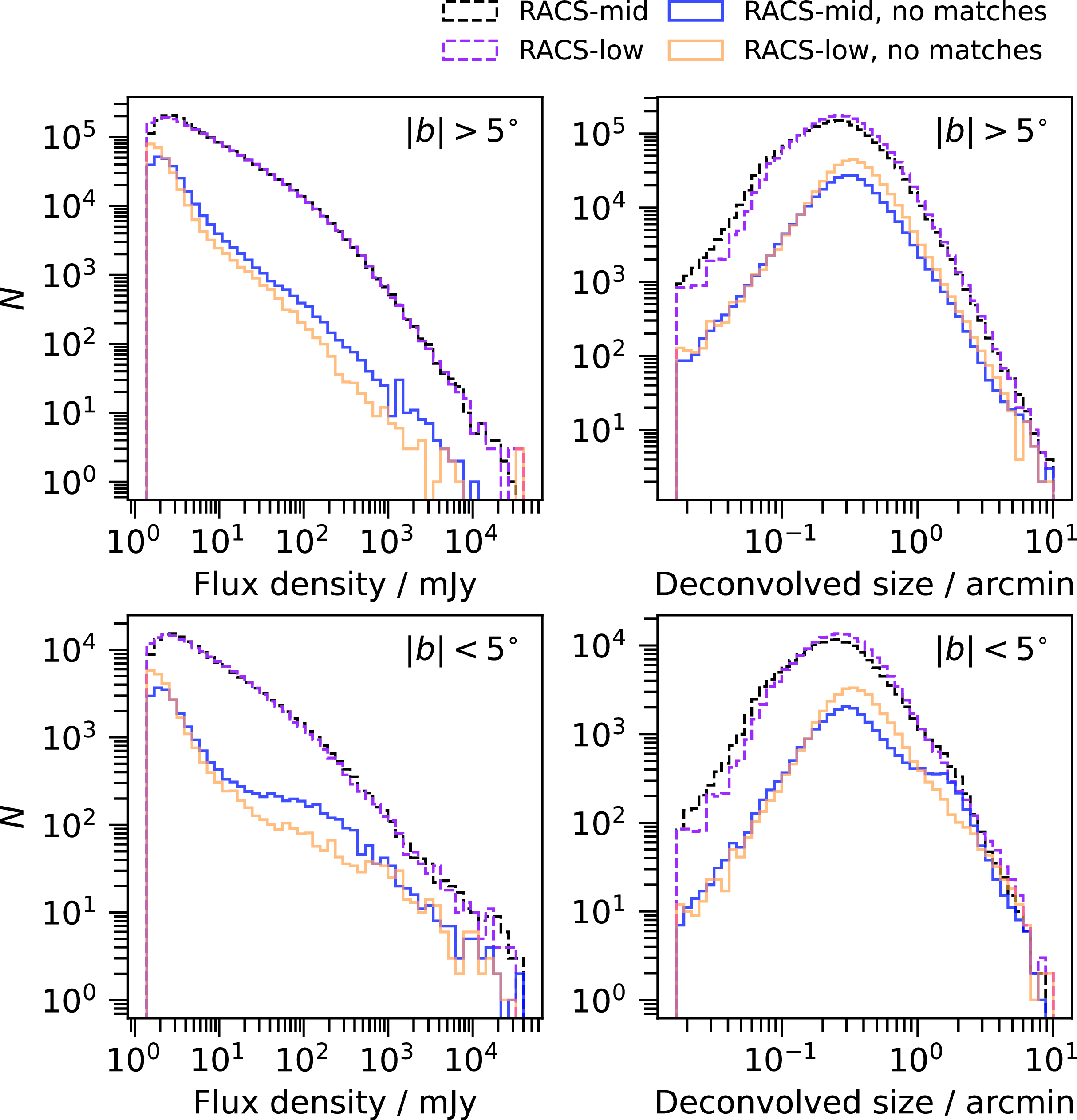
Figure 17. The distribution of sources as a function of flux density (top) and fitted major axis (bottom) for the RACS-mid 25-arcsec catalogue and the RACS-low catalogue. Left. Sources outside of the Galactic Plane ( $|b|>5^{\circ}$
). Right. Sources within the Galactic Plane (
$|b|>5^{\circ}$
). Right. Sources within the Galactic Plane ( $|b|<5^{\circ}$
). The distribution of sources that are not cross-matched between the two catalogues are also shown.
$|b|<5^{\circ}$
). The distribution of sources that are not cross-matched between the two catalogues are also shown.
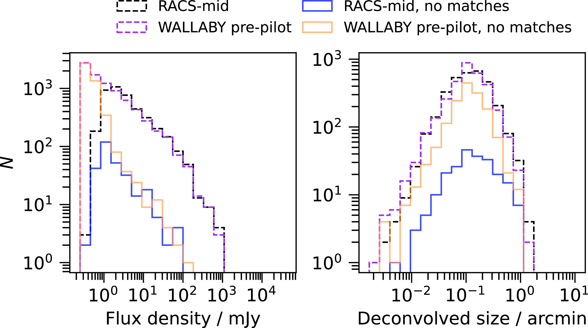
Figure 18. As in Fig. 17, comaparing the RACS-mid primary catalogue to the WALLABY pre-pilot catalogue (only considering sources within the WALLABY pre-pilot image region). No Galactic Plane cut is applied as the region is not within the Galactic Plane.
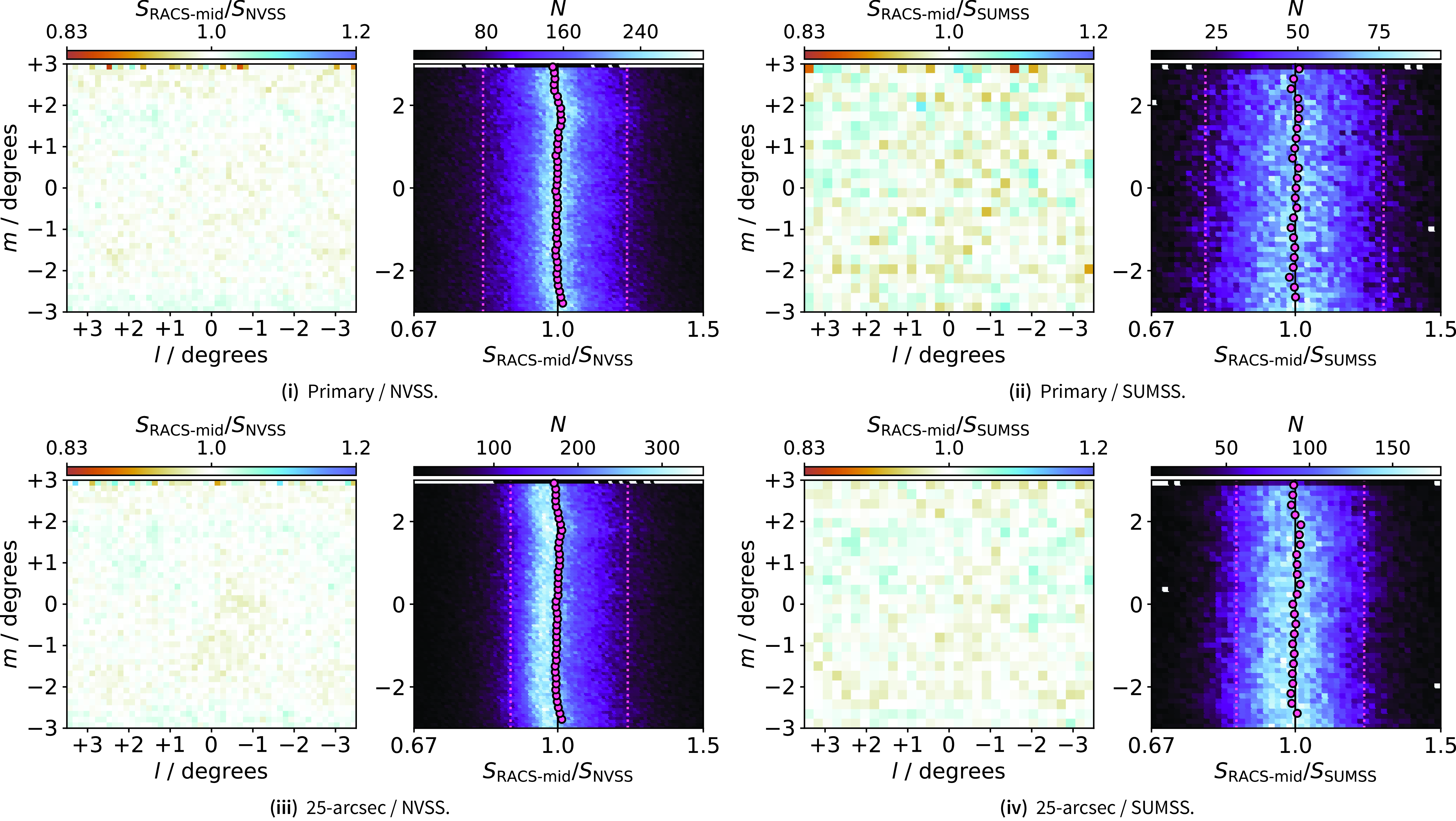
Figure 19. Brightness scale comparison as a function of tile reference coordinates for the primary catalogue and NVSS (i) and SUMSS (ii), and the 25-arcsec catalogue and NVSS (iii) and SUMSS (iv). Left. Median-binned flux density ratios. Right. 2D histogram of the flux density ratios and the tile coordinate m, with medians in m show as pink circles. $16\text{th}$
and
$16\text{th}$
and $84\text{th}$
percentiles are shown as pink, dashed lines.
$84\text{th}$
percentiles are shown as pink, dashed lines.
For assessing the brightness scale across the survey images, we apply the same unresolved flags described in Section 4.4 to the individual source lists then cross-match the individual sources lists to the various external catalogues as described in Section 4.8. Note that more sources will be cross-matched in this per–source list assessment than when looking at the full catalogues, since we include sources in at the edge of images in overlap regions. For assessing the brightness scale, we look at the SUMSS and NVSS cross-matches to allow easy reference to the same comparisons made in Reference DuchesnePaper IV for the original images. As part of the additional metadata added prior to source list concatenation, we add tile-reference coordinates, (l,m), for each source entry. In the case of the mosaicked images, these (l,m) values are with reference to the mosaiced image, and not the original image that was used in the mosaic. Following Reference DuchesnePaper IV we then median-bin the flux density ratios ( $S_{\text{RACS-mid}}/S_{\text{survey}}$
, for NVSS and SUMSS) in bins of angular sizes
$S_{\text{RACS-mid}}/S_{\text{survey}}$
, for NVSS and SUMSS) in bins of angular sizes $8.6 \times 8.6$
arcmin
$8.6 \times 8.6$
arcmin $^{2}$
(NVSS) and
$^{2}$
(NVSS) and $14.4 \times 14.4$
arcmin
$14.4 \times 14.4$
arcmin $^{2}$
(SUMSS).
$^{2}$
(SUMSS).
Fig. 19(i)–19(iv) shows (left) the flux density ratios of sources in the RACS-mid catalogues and comparison catalogues, median-binned in the image-based (l, m) coordinates. Fig. 19 also shows the 2D histogram of flux density ratios in m, where the majority of the edge-effects were seen in Reference DuchesnePaper IV. We normalise the ratios by the overall median flux density ratio to ensure bulk offsets introduced by a choice of spectral index do not detract from position-dependent effects. For both the primary and 25-arcsec catalogues, position-dependent brightness effects are almost completely removed due to the mosaicking process. Specifically, we refer to Figures 30 and 31 in Reference DuchesnePaper IV that highlight these residual brightness scales features. Residual variation in the mosaiced images is $\lesssim$
a few %.
$\lesssim$
a few %.
With the reduction of edge effects, we determine that the brightness scale uncertainty for the primary and 25-arcsec catalogues retain the uncertainty reported for the central tile region in Reference DuchesnePaper IV: 6%. The time-domain catalogue retains both uncertainties (6% and 14% for the tile edges, Equation (5) in Reference DuchesnePaper IV), and the source entries will explicitly note the appropriate uncertainty based on its position in the image it is taken from.
5. Data availability
Paper IV describes the raw survey data and how to access the original images and calibrated visibility datasets. This data release comprises both the full-sensitivity mosaicked images used for the primary catalogue and the fixed-resolution 25-arcsec catalogue, as well as the three catalogues described in Section 3. For the catalogues and full-sensitivity images described in this paper, availability is similarly through the CASDAFootnote 16 (Chapman et al. Reference Chapman, Dempsey, Miller, Heywood, Pritchard, Sangster, Whiting, Dart, Lorente, Shortridge and Wayth2017; Huynh et al. Reference Huynh, Dempsey, Whiting, Ophel, Ballester, Ibsen, Solar and Shortridge2020), and each product is summarised here for completeness:
Primary catalogue.
-
Source list. The final merged source lists. This contains all sources detected during source-finding on the full-sensitivity images that are not removed due to the de-duplication process when constructing the catalogue. This catalogue features the full sky up to
$\delta_{\text{J2000}} = +49^{\circ}$
with sources detected in Stokes I images. This is the recommended catalogue for most use cases. -
Component list. The Gaussian components associated with the source list. Generally only used for reconstruction of the source models.
-
Full-sensitivity images. Stokes I full-sensitivity images with associated weight maps. For most use-cases these are the preferred images to use over the original images.
-
Link to images and catalogues.

Auxiliary 25-arcsec catalogue.
-
Source list. The merged 25-arcsec source lists. This is similar to the primary catalogue, except with the fixed 25-arcsec resolution and with coverage up to
$\delta_{\text{J2000}} = +30^{\circ}$
. -
Component list. The Gaussian components associated with the 25-arcsec source list.
-
Full-sensitivity 25-arcsec images. Stokes I full-sensitivity images with associated weight maps.
-
Link for images and catalogues.

Auxiliary time-domain catalogue.
-
Source list. The concatenated source list from the original RACS-mid images. This covers the entire survey region, and retains duplicate source entries.
-
Component list. The Gaussian components associated with the time-domain source list.
-
Link to the catalogues.
6. Summary
The ASKAP has completed observing the sky in three bands centred at 887.5, 1 367.5, and 1 632.5 MHz as part of the RACS. RACS-low (at 887.5 MHz) and RACS-mid (at 1 367.5 MHz) have been processed and released (Reference McConnellPaper I; Reference DuchesnePaper IV) with a catalogue for RACS-low also released (Reference HalePaper II). While the 1 632.5-MHz data have been observed, these data are yet to be processed and will be released in the future as RACS-high. This work describes the release of an ‘all-sky’ general-purpose catalogue for RACS-mid, along with two auxiliary catalogues for more specific use-cases.
The general purpose, primary catalogue was created by mosaicking nearby images to improve sensitivity in overlapping regions, convolving to the lowest common resolution of neighbouring images, source-finding with PyBDSF on these full-sensitivity mosaics, then merging the output source lists while removing duplicate entries. The primary catalogue covers $-90^{\circ} < \delta_{\text{J2000}} \leq +49^{\circ}$
(
$-90^{\circ} < \delta_{\text{J2000}} \leq +49^{\circ}$
( $\sim$ $36\,200$
deg
$36\,200$
deg $^2$
) and contains 3 107 143 sources (2 863 400 excluding the Galactic Plane) down to
$^2$
) and contains 3 107 143 sources (2 863 400 excluding the Galactic Plane) down to $5\sigma_{\text{rms}}$
. We investigated the reliability and completeness of the catalogues, finding a significant decrease in reliability in the Galactic Plane due to higher incidence of artefacts from extended sources. The primary catalogue is found to be 95% complete at 2 mJy. We matched the catalogue to other external catalogues such as RACS-low, LoTSS-DR2, VLASS-QL, SUMSS, NVSS, and FIRST and find properties such as flux density and astrometry consistent with what is reported in Reference DuchesnePaper IV, suggesting additional mosaicking done here is not introducing extra systematic issues into the images and catalogue.
$5\sigma_{\text{rms}}$
. We investigated the reliability and completeness of the catalogues, finding a significant decrease in reliability in the Galactic Plane due to higher incidence of artefacts from extended sources. The primary catalogue is found to be 95% complete at 2 mJy. We matched the catalogue to other external catalogues such as RACS-low, LoTSS-DR2, VLASS-QL, SUMSS, NVSS, and FIRST and find properties such as flux density and astrometry consistent with what is reported in Reference DuchesnePaper IV, suggesting additional mosaicking done here is not introducing extra systematic issues into the images and catalogue.
In addition to the primary catalogue, we also provide an auxiliary version of the catalogue with a fixed resolution of $25^{\prime\prime} \times 25^{\prime\prime}$
. This catalogue is created in a similar way to the primary catalogue, except images are all convolved to
$25^{\prime\prime} \times 25^{\prime\prime}$
. This catalogue is created in a similar way to the primary catalogue, except images are all convolved to $25^{\prime\prime} \times 25^{\prime\prime}$
prior to mosaicking and source-finding. Because of this, the coverage is reduced to
$25^{\prime\prime} \times 25^{\prime\prime}$
prior to mosaicking and source-finding. Because of this, the coverage is reduced to $\delta_{\text{2000}} \leq +30^{\circ}$
. This matches closely the existing RACS-low catalogue described in Reference HalePaper II. This 25-arcsec catalogue features lessened sensitivity and consequently fewer sources—2 156 393 sources above
$\delta_{\text{2000}} \leq +30^{\circ}$
. This matches closely the existing RACS-low catalogue described in Reference HalePaper II. This 25-arcsec catalogue features lessened sensitivity and consequently fewer sources—2 156 393 sources above $5\sigma_{\text{rms}}$
(1 992 406 excluding the Galactic Plane)—with a significant decrease in reliability in the Galactic Plane. Other properties and comparisons are similar to the primary catalogue.
$5\sigma_{\text{rms}}$
(1 992 406 excluding the Galactic Plane)—with a significant decrease in reliability in the Galactic Plane. Other properties and comparisons are similar to the primary catalogue.
A third auxiliary catalogue is provided for time-domain science. This version features no additional convolution or mosaicking of images prior to source-finding and retains all duplicate source entries in overlapping regions. The purpose of this auxiliary time-domain catalogue is to detect and characterise time-variable sources without averaging signal between epochs as will be the case for some sources in the primary catalogue.
All data products, including catalogues and full-sensitivity images are being made available through the CASDA. This data release focuses on total intensity with Stokes I and work is currently underway to catalogue the sources of circular polarisation using the Stokes V images produced as part of RACS-mid (e.g. Rose et al. Reference Rose2023).
Acknowledgement
We would like to thank the anonymous referee for their feedback that has improved the quality of this work. This scientific work uses data obtained from Inyarrimanha Ilgari Bundara/the Murchison Radio-astronomy Observatory. We acknowledge the Wajarri Yamaji People as the Traditional Owners and native title holders of the Observatory site. CSIRO’s ASKAP radio telescope is part of the Australia Telescope National Facility (https://ror.org/05qajvd42). Operation of ASKAP is funded by the Australian Government with support from the National Collaborative Research Infrastructure Strategy. ASKAP uses the resources of the Pawsey Supercomputing Research Centre. Establishment of ASKAP, Inyarrimanha Ilgari Bundara, the CSIRO Murchison Radio-astronomy Observatory and the Pawsey Supercomputing Research Centre are initiatives of the Australian Government, with support from the Government of Western Australia and the Science and Industry Endowment Fund.
We used a range of python software packages during this work and the production of this manuscript, including aplpy (Robitaille & Bressert Reference Robitaille and Bressert2012), astropy (Astropy Collaboration et al. 2018), matplotlib (Hunter Reference Hunter2007), numpy (Harris et al. 2020), scipy (Virtanen et al. Reference Virtanen2020), and cmasher (van der Velden Reference van der Velden2020). Some of the results in this paper have been derived using the healpy (Zonca et al. Reference Zonca, Singer, Lenz, Reinecke, Rosset, Hivon and Gorski2019) and HEALPix package. We make use of ds9 (Joye & Mandel Reference Joye, Mandel, Payne, Jedrzejewski and Hook2003) and topcat (Taylor Reference Taylor, Shopbell, Britton and Ebert2005) for visualisation, as well as the ‘Aladin sky atlas’ developed at CDS, Strasbourg Observatory, France (Bonnarel et al. Reference Bonnarel2000; Boch & Fernique Reference Boch, Fernique, Manset and Forshay2014) for obtaining catalogue data. For precision rounding in LaTeX tables we used to-precision: https://bitbucket.org/william_rusnack/to-precision/src/master/.
This project used public archival data from the Dark Energy Survey (DES). Funding for the DES Projects has been provided by the US Department of Energy, the US National Science Foundation, the Ministry of Science and Education of Spain, the Science and Technology Facilities Council of the United Kingdom, the Higher Education Funding Council for England, the National Center for Supercomputing Applications at the University of Illinois at Urbana-Champaign, the Kavli Institute of Cosmological Physics at the University of Chicago, the Center for Cosmology and Astro-Particle Physics at the Ohio State University, the Mitchell Institute for Fundamental Physics and Astronomy at Texas A&M University, Financiadora de Estudos e Projetos, Fundação Carlos Chagas Filho de Amparo à Pesquisa do Estado do Rio de Janeiro, Conselho Nacional de Desenvolvimento Científico e Tecnológico and the Ministério da Ciência, Tecnologia e Inovação, the Deutsche Forschungsgemeinschaft, and the Collaborating Institutions in the Dark Energy Survey. The Collaborating Institutions are Argonne National Laboratory, the University of California at Santa Cruz, the University of Cambridge, Centro de Investigaciones Energéticas, Medioambientales y Tecnológicas-Madrid, the University of Chicago, University College London, the DES-Brazil Consortium, the University of Edinburgh, the Eidgenössische Technische Hochschule (ETH) Zürich, Fermi National Accelerator Laboratory, the University of Illinois at Urbana-Champaign, the Institut de Ciències de l’Espai (IEEC/CSIC), the Institut de Física d’Altes Energies, Lawrence Berkeley National Laboratory, the Ludwig-Maximilians Universität München and the associated Excellence Cluster Universe, the University of Michigan, the National Optical Astronomy Observatory, the University of Nottingham, The Ohio State University, the OzDES Membership Consortium, the University of Pennsylvania, the University of Portsmouth, SLAC National Accelerator Laboratory, Stanford University, the University of Sussex, and Texas A&M University. Based in part on observations at Cerro Tololo Inter-American Observatory, National Optical Astronomy Observatory, which is operated by the Association of Universities for Research in Astronomy (AURA) under a cooperative agreement with the National Science Foundation.
The Digitized Sky Surveys were produced at the Space Telescope Science Institute under US Government grant NAG W-2166. The images of these surveys are based on photographic data obtained using the Oschin Schmidt Telescope on Palomar Mountain and the UK Schmidt Telescope. The plates were processed into the present compressed digital form with the permission of these institutions.
Appendix A. Catalogue columns
While the columns (both names and data) are similar to those used for the RACS-low catalogue (see Section 4.3 in Reference HalePaper II). Tables A1 and A2 outline the catalogues columns used for the three RACS-mid source and component catalogues, respectively. Note that the source and component lists feature almost identical columns with the exception of Source_ID (in the source list) and Gaussian_ID (in the component list) for unique identifiers for sources and components, respectively. The consequence of this is that quantity columns such as Total_flux correspond to the source in source list or the component in the component list.
Some columns have information that refers to the original images (SBID, Scan_start_MJD, and Scan_length). In the case of the main reference catalogue and auxiliary 25-arcsec catalogue these refer to the central image that was used in mosaicking but does not include information about neighbouring images included in the mosaic. Therefore these columns will likely be accurate for sources at the centre (i.e. with low Tile_sep) but will not be accurate towards image edges. In the case of the auxiliary time-domain catalogue, sources are taken from only non-mosaicked images so these columns will be accurate for all sources.
Tables A3 and A4 show three example rows from the primary source catalogue and primary component catalogue, respectively. The three example rows are 0, 500 000, and 1 500 000, chosen arbitrarily.
Table A1. Columns in the RACS-mid source catalogues.

Table A2. Columns in the RACS-mid component catalogues.

Table A3. Example three rows from the primary catalogue source list. Rows with associated uncertainties are rounded to match the uncertainty.

Table A4. Example three rows from the primary catalogue component list. Rows with associated uncertainties are rounded to match the uncertainty.
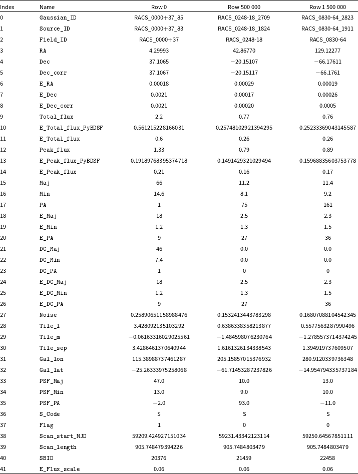


 Open access