


1. Introduction
The physics of neutron stars represents a great challenge to test our understanding of matter under extreme conditions. The huge variation of the density from the star surface (ρ ~ 10 g/cm3) to its centre (ρ ~ 1015 g/cm3) requires the modelling of systems in very different physical conditions like heavy neutron-rich nuclei arranged to form a lattice structure as in the outer crust of the star, or a system of strong interacting hadrons (nucleons, and possibly hyperons or a phase with deconfined quarks) to form a quantum fluid as in the stellar core (Prakash et al. Reference Prakash, Bombaci, Prakash, Ellis, Lattimer and Knorren1997). The description of such a variety of nuclear systems needs a considerable theoretical effort and a knowledge as much as possible accurate of the interactions between the constituents present inside the star. The bulk properties of neutron stars (e.g. mass, radius, mass-shed frequency) chiefly depend on the equation of state (EOS) describing the macroscopic properties of stellar matter. The EOS of dense matter is also a basic ingredient for modelling various astrophysical phenomena related to neutron stars, as core-collapse supernovae (SNe) (Oertel et al. Reference Oertel, Hempel, Klahn and Typel2017) and binary neutron star (BNS) mergers (Bauswein & Janka Reference Bauswein and Janka2012; Bernuzzi, Dietrich, & Nagar Reference Bernuzzi, Dietrich and Nagar2015; Sekiguchi et al. Reference Sekiguchi, Kiuchi, Kyutoku, Shibata and Taniguchi2016; Rezzolla & Takami Reference Rezzolla and Takami2016). We note, however, that in order to perform realistic numerical simulations for the latter two cases, the inclusion of thermal contributions is very important. The very recent detection of gravitational waves from a binary neutron star merger (GW170817) by the LIGO–Virgo collaboration (Abbott et al. Reference Abbott2017) has strongly increased the interest to these astrophysical phenomena and more in general to dense matter physics.
In the present work, we model the core of neutron stars as a uniform charge neutral fluid made of neutrons, protons, electrons, and muons in equilibrium with respect to the weak interaction. Such system is well known in literature as β-stable nuclear matter. In addition, we also consider the possible formation of hyperons in the inner core of neutron stars. Accordingly, we calculate various neutron star properties making use of an EOS for the stellar core obtained within a microscopic non-relativistic approach based on the Brueckner–Bethe–Goldstone (BBG) many-body theory and adopting the Brueckner–Hartree–Fock (BHF) approximation (Day Reference Day1967; Baldo & Burgio Reference Baldo and Burgio2012). In such a microscopic approach, the only inputs required are the bare two- and three-body nuclear interactions derived in vacuum using nucleon–nucleon (NN) scattering data and information (binding energies and scattering observables) on light (atomic mass number A = 3, 4) nuclei.
It is well known that three-nucleon forces (TNFs) play a very important role in nuclear physics. For example, TNFs are required to reproduce the experimental binding energy of few-nucleon (A = 3, 4) systems (Kalantar-Nayestanaki et al. Reference Kalantar-Nayestanaki, Epelbaum, Messchendorp and Nogga2012). TNFs are also essential to reproduce the empirical saturation point (n 0 = 0.16 ± 0.01 fm−3,  $E/A{|_{{n_0}}} = - 16.0 \pm 1.0 {\rm{MeV}}$) of symmetric nuclear matter (SNM) and to give an adequately stiff EOS which is consistent with present measured neutron star masses and in particular with the mass M = 2.01 ± 0.04M⊙ (Antoniadis et al. Reference Antoniadis2013) of the neutron star in PSR J0348+0432.
A modern and very powerful approach (Weinberg Reference Weinberg1979) to derive two- as well as many-body nuclear interactions is the one provided by chiral effective field theory (see Epelbaum, Hammer, & Meißner (Reference Epelbaum, Hammer and Meißner2009) and Machleidt & Entem (Reference Machleidt and Entem2011) for a detailed review). In this method two-, three-, as well as many-body nuclear interactions can be calculated order by order according to a well-defined procedure based on a low-energy effective quantum chromodynamics (QCD) Lagrangian. This Lagrangian is built in such a way to keep the main symmetries of QCD and in particular the approximate chiral symmetry. The starting point of this chiral perturbation theory (ChPT) is the definition of a power counting in the ratio Q/Ʌχ, where Q denotes a low-energy scale which can be identified with the momentum of the external nucleons or with the pion mass mπ. Ʌχ ~ 1 GeV is the so-called chiral symmetry breaking scale which sets up the energy range of validity of the theory. In this effective field theory, the details of the QCD dynamics are enclosed in the so-called low-energy constants (LECs), which are parameters fitted using experimental data such as scattering data and binding energies of light nuclei. This well-defined scheme is very advantageous in the case of nucleonic systems where it has been shown that TNFs play a very important role (Kalantar-Nayestanaki et al. Reference Kalantar-Nayestanaki, Epelbaum, Messchendorp and Nogga2012).
In this work, we present some microscopic calculations of the EOS of β-stable neutron star matter using the chiral potentials derived by Ekström et al. (Reference Ekström, Jansen, Wendt, Hagen, Papenbrock, Bacca, Carlsson and Gazit2014) at the next-to-next-to-leading order (N2LO) of ChPT. Interactions derived in ChPT have been calculated even at higher order like N3LO and N4LO (Entem et al. Reference Entem, Kaiser, Machleidt and Nosyk2015; Epelbaum, Krebs, & Meißner Reference Epelbaum, Krebs and Meißner2015). One of the problems to perform nuclear structure and nuclear matter calculations at a fixed order higher than N2LO is that the number of many-body contributions proliferates very quickly increasing the order of the expansion. Therefore, it turns out prohibitive to take into account all the contributions arising at a given arbitrary order of ChPT. Conversely at the order N2LO, it has been shown by Ekström et al. (Reference Ekström, Jansen, Wendt, Hagen, Papenbrock, Bacca, Carlsson and Gazit2014) that it is possible to derive an NN potential with a χ 2/datum ∼ 1, as well as to take into account leading-order TNFs. Previous versions of NN potentials at N2LO based on traditional fit techniques of the experimental data provided a χ 2/datum ∼ 10, and therefore, they were not enough accurate to be used in practical calculations. Alternatively Ekström et al. (Reference Ekström, Jansen, Wendt, Hagen, Papenbrock, Bacca, Carlsson and Gazit2014) used a new optimisation technique based on the algorithm POUNDerS (Practical Optimization Using No Derivatives for sum of Squares) (Kortelainen et al. Reference Kortelainen, Lesinski, More, Nazarewicz, Sarich, Schunck, Stoitsov and Wild2010) which drastically improved the quality of the data fit. Thus at N2LO all the contributions emerging from ChPT can be consistently included in a many-body calculation.
2. Chiral nuclear interactions
As we have already discussed previously, in the present work we employ two different interactions derived in ChPT both for two- and the three-body sectors. We adopt indeed an NN potential calculated at N2LO supplemented by a TNF calculated at the same order. More specifically as a two-body nuclear interaction, we have used the optimised chiral potentials proposed by Ekström et al. (Reference Ekström, Jansen, Wendt, Hagen, Papenbrock, Bacca, Carlsson and Gazit2014). We have already pointed out that all the possible operators contributing to the NN potential as well as leading-order TNFs arise at N2LO of ChPT. Thus, it is possible to understand several properties of nuclear structure at this order of the perturbative expansion. The optimised parameters of the NN potential fitted at N2LO are the constants c 1, c 3, and c 4 coming from the pion-nucleon (πN) Lagrangian, plus 11 partial waves from contact terms.
The chiral NN interaction by Ekström et al. (Reference Ekström, Jansen, Wendt, Hagen, Papenbrock, Bacca, Carlsson and Gazit2014) has been optimised to the proton–proton and the proton–neutron scattering data for laboratory scattering energies below 125 MeV, and to deuteron observables. The N2LO TNF has been then fixed requiring to reproduce the 3H half-life and the binding energies of 3H and 3He nuclei. The total (i.e. two-body plus three-body) interaction has been then used to predict the Gamow–Teller transition matrix elements in 14C and 22,24O nuclei using consistent two-body currents. In their paper Ekström et al. (Reference Ekström, Jansen, Wendt, Hagen, Papenbrock, Bacca, Carlsson and Gazit2014) provided three different versions of this interaction according to three different values of the cut-off Ʌ = 450, 500, 550 MeV used to regularise the short-range part of the potentials. The χ 2/datum of the NN interaction varied from 1.33 to 1.18 passing from Ʌ = 450 to Ʌ = 550 MeV. In the present work we have adopted the model with Ʌ = 550 MeV hereafter referred to as the N2LOopt NN potential. We have checked, however, that similar results could be obtained also using the other models reported in Ekström et al. (Reference Ekström, Jansen, Wendt, Hagen, Papenbrock, Bacca, Carlsson and Gazit2014).
Concerning the form of the TNF, we have used the non-local N2LO version given by Epelbaum et al. (Reference Epelbaum, Nogga, Glöckle, Kamada, Meißner and Witała2002). The non-locality of the N2LO TNF depends only on the particular form of the cut-off used to regularise short-range part of the potential. It reads:
 $$V_{3N}^{(2\pi\kern-.6pt)} = \sum_{i\neq j\neq k} \frac{g_A^2}{8f_\pi^4}
\frac{\boldsymbol{\sigma}_i \cdot \textbf{\textit{{q}}}_i \, \boldsymbol{\sigma}_j \cdot
\textbf{\textit{q}}_j}{({\textbf{\textit{q}}_{\textbf{\textit{i}}}}^2 + m_\pi^2)({\textbf{\textit{q}}_{\textbf{\textit{i}}}}^2+m_\pi^2)}
f_{ijk}^{\,\alpha \beta}\tau_i^\alpha \tau_j^\beta,$$
$$V_{3N}^{(2\pi\kern-.6pt)} = \sum_{i\neq j\neq k} \frac{g_A^2}{8f_\pi^4}
\frac{\boldsymbol{\sigma}_i \cdot \textbf{\textit{{q}}}_i \, \boldsymbol{\sigma}_j \cdot
\textbf{\textit{q}}_j}{({\textbf{\textit{q}}_{\textbf{\textit{i}}}}^2 + m_\pi^2)({\textbf{\textit{q}}_{\textbf{\textit{i}}}}^2+m_\pi^2)}
f_{ijk}^{\,\alpha \beta}\tau_i^\alpha \tau_j^\beta,$$
 $$V_{3N}^{(1\pi\kern-.6pt)} = -\sum_{i\neq j\neq k}
\frac{g_A c_D}{8f_\pi^4 \Lambda_\chi} \frac{\boldsymbol{\sigma}_j \cdot \textbf{\textit{q}}_j}{\textbf{\textit{q}}_{\textbf{\textit{j}}}^2+m_\pi^2}
\boldsymbol{\sigma}_i \cdot
\textbf{\textit{q}}_j \, {\boldsymbol \tau}_i \cdot {\boldsymbol \tau}_j,$$
$$V_{3N}^{(1\pi\kern-.6pt)} = -\sum_{i\neq j\neq k}
\frac{g_A c_D}{8f_\pi^4 \Lambda_\chi} \frac{\boldsymbol{\sigma}_j \cdot \textbf{\textit{q}}_j}{\textbf{\textit{q}}_{\textbf{\textit{j}}}^2+m_\pi^2}
\boldsymbol{\sigma}_i \cdot
\textbf{\textit{q}}_j \, {\boldsymbol \tau}_i \cdot {\boldsymbol \tau}_j,$$
 $$V_{3N}^{(\rm ct)} = \sum_{i\neq j\neq k} \frac{c_E}{2f_\pi^4 \Lambda_\chi}
{\boldsymbol \tau}_i \cdot {\boldsymbol \tau}_j,$$
$$V_{3N}^{(\rm ct)} = \sum_{i\neq j\neq k} \frac{c_E}{2f_\pi^4 \Lambda_\chi}
{\boldsymbol \tau}_i \cdot {\boldsymbol \tau}_j,$$
where  $\textbf{\textit{q}}_i=\textbf{\textit{p}}_{\textbf{\textit{i}}}^{\prime}-\textbf{\textit{p}}_i$ is the difference between the final and initial momentum of nucleon i and
 $$f_{ijk}^{\alpha \beta} = \delta^{\alpha \beta}\big(-4c_1m_\pi^2 + 2c_3 \textbf{\textit{q}}_i \cdot \textbf{\textit{q}}_j\big) + c_4 \epsilon^{\alpha \beta \gamma} \tau_k^\gamma \boldsymbol{\sigma}_k \cdot\big(\textbf{\textit{q}}_i \times \textbf{\textit{q}}_j\big).$$
In equations (1)–(4) σi and τi are the Pauli matrices which act on the spin and isospin spaces, while gA = 1.29 is the axial-vector coupling and fπ = 92.4 MeV the pion decay constant. The labels i, j, k run over the values 1, 2, 3, which take into account all the six possible permutations in each sum. In equation (4) c 1, c 3, c 4, cD, and cE denote the so-called LECs. We note that c 1, c 3, and c 4 are already fixed at two-body level by the πN Lagrangian; therefore, they do not represent free parameters. In Table 1 we report the values of ci that we have adopted in the present work. The last two parameters cD and cE are not fixed by the data from two-body scattering and have to be set up using some specific observable in finite nuclei or in infinite nuclear matter. In the present work we have explored both the possibilities. In the following the TNF fitted by Ekström et al. (Reference Ekström, Jansen, Wendt, Hagen, Papenbrock, Bacca, Carlsson and Gazit2014) to reproduce the properties of light nuclei will be denoted as the N2LO TNF, whereas the parametrisation fitted to provide a good saturation point of SNM will be denoted as the N2LO1 TNF.
Table 1. Values of the LECs of the two TNF parametrisations used in the present work
For the two parametrisations we have set a cut-off of 550 MeV. cD and cE are dimensionless whereas c 1, c 3, and c 4 are expressed in GeV−1.
Finally, we have multiplied the whole interaction by a non-local cut-off of the form:
 $$F_\Lambda(\textbf{\textit{p}}, \textbf{\textit{q}})={\rm exp}\left[-\left(\frac{4 \textbf{\textit{p}}^2+3 \textbf{\textit{q}}^2}{4 \Lambda^2}\right)^n\right]\kern-1.5pt.$$
This allows to regularise the short part of the interaction which is not correctly described by ChPT and it is sensible to the internal structure of nucleons. In equation (5): p = (p 1 – p 2)/2 and q = 2/3[p 3 –(p 1 – p 2)]. Finally, following Ekström et al. (Reference Ekström, Jansen, Wendt, Hagen, Papenbrock, Bacca, Carlsson and Gazit2014), in the present work, we have set Λ = 550 MeV and n = 2.
3. The BHF approach with three-body forces
The BBG many-body theory (Day Reference Day1967; Baldo & Burgio Reference Baldo and Burgio2012) allows to calculate the ground state of nuclear matter in terms of the so-called hole-line expansion. The different diagrams which contribute to the energy of the system are grouped according to the number of independent hole-lines, where the hole-lines represent empty single particle states in the Fermi sea. The lowest order the BBG theory is the so-called BHF approximation. In the present work we have performed all the calculations in such framework. The starting point of the BHF approach is the calculation of the so-called G-matrices which describe the interaction between two nucleons taking into account the presence of all the surrounding nucleons of the medium; these nucleons restrict the possible final states of the NN scattering.
For asymmetric nuclear matter with total nuclear density ρ = ρn + ρp and isospin asymmetry β = (ρn − ρp)/ρ (being, ρn and ρp the neutron and proton densities), one has to consider three different G-matrices for the nn-, np-, and pp-channels. These G-matrices are obtained solving the well-known Bethe–Goldstone equation:
 $$G_{\tau \tau'}(\omega) = V_{\tau \tau'} + \sum_{k, k'} V_{\tau \tau'} \frac{\mid\textbf{\textit{k}},\textbf{\textit{k}}^{\boldsymbol{\prime}}\rangle \, Q_{\tau \tau'}\, \langle\textbf{\textit{k}},\textbf{\textit{k}}^{\boldsymbol{\prime}}\mid}{\omega-\epsilon_{\tau}(k)-\epsilon_{\tau'}(k') + i\varepsilon} G_{\tau \tau'}(\omega),$$
where τ, τ′ = n, p are isospin indices, Vττ ′ denotes the bare NN interaction in a given NN channel, |k, k′〉Qττ ′〈k, k′| is the Pauli operator which projects the intermediate nucleons states out of the Fermi sphere. In this way the Pauli exclusion principle is automatically satisfied. ω is the so-called starting energy which is given by the sum of energies of the interacting nucleons in a non-relativistic approximation. The single-particle energy ɛτ(k) of a nucleon with momentum k and mass mτ is given by
 $${\varepsilon _\tau }(k) = \frac{{{\hbar ^2}{k^2}}}{{2{m_\tau }}} + {U_\tau }(k),$$
where the single-particle potential Uτ(k) is the mean field felt by one nucleon due to the interactions with the other nucleons of the medium. In the BHF approximation, Uτ(k) is given by the real part of the Gττ ′-matrix calculated on energy shell:
 $$U_\tau(k) =\sum_{\tau'=n,p}\ \sum_{k'\le k_{F_{\tau'}}} \mbox{Re} \ \langle \textbf{\textit{k}} \textbf{\textit{k}}^{\boldsymbol{\prime}}
\mid G_{\tau \tau'}(\omega=\omega^*) \mid \textbf{\textit{k}} \textbf{\textit{k}}^{\boldsymbol{\prime}}\rangle_A,$$
$$U_\tau(k) =\sum_{\tau'=n,p}\ \sum_{k'\le k_{F_{\tau'}}} \mbox{Re} \ \langle \textbf{\textit{k}} \textbf{\textit{k}}^{\boldsymbol{\prime}}
\mid G_{\tau \tau'}(\omega=\omega^*) \mid \textbf{\textit{k}} \textbf{\textit{k}}^{\boldsymbol{\prime}}\rangle_A,$$
where ω* = ɛτ(k) + ɛτ ′(k′) and the sum runs over all neutron and proton occupied states and the matrix elements are antisymmetrised. In the solution of the Bethe–Goldstone equation, we have employed the so-called continuous choice (Jeukenne, Lejeunne, & Mahaux Reference Jeukenne, Lejeunne and Mahaux1967; Grangé, Cugnon, & Lejeune Reference Grangé, Cugnon and Lejeune1987) for the single-particle potential Uτ(k). It has been shown in Refs. Song et al. (Reference Song, Baldo, Giansiracusa and Lombardo1998); Baldo et al. (Reference Baldo, Giansiracusa, Lombardo and Song2000) that the contribution to the energy per particle E/A from the diagrams coming from the three hole-lines is strongly minimised using this prescription. Consequently, a faster convergence of the hole-line expansion for E/A is achieved (Song et al. Reference Song, Baldo, Giansiracusa and Lombardo1998; Baldo et al. Reference Baldo, Bombaci, Giansiracusa and Lombardo1990, Reference Baldo, Giansiracusa, Lombardo and Song2000) when compared to the so-called gap choice for Uτ(k), where the single-particle potential is set to zero above the Fermi momentum.
Equations (6)–(8) are solved in a self-consistent way and then the energy per particle is calculated as
 $$\frac{E}{A}(\rho ,\beta ) = \frac{1}{A}\sum\limits_{\tau = n,p} \sum\limits_{k \le {k_{{F_\tau }}}} \left( {\frac{{{\hbar ^2}{k^2}}}{{2{m_\tau }}} + \frac{1}{2}{U_\tau }(k)} \right).$$
From the energy per particle, all the other relevant quantities can be calculated using standard thermodynamical relations.
3.1. Inclusion of TNFs in the BHF approach
Non-relativistic quantum many-body approaches are not able to reproduce the empirical saturation point of SNM: ρ 0 = 0.16 ± 0.01 fm−3,  $E/A{|_{{\rho _0}}} = - 16.0 \pm 1.0 {\rm{MeV}}$. Several studies employing a large variety of different NN potentials have indeed shown that the saturation points lie inside a narrow band known in literature as Coester band (Coester et al. Reference Coester, Cohen, Day and Vincent1970; Day Reference Day1981). The various models showed either a too large saturation density or a too small value for the energy per particle with respect to the empirical value. A similar behaviour has been also found for the binding energies of finite nuclei where the ground states turned out to be too large or too small when compared to the experimental ones. The inclusion of TNFs allows to improve the description of both SNM nuclear matter (Friedman & Pandharipande Reference Friedman and Pandharipande1981; Baldo, Bombaci, & Burgio Reference Baldo, Bombaci and Burgio1997; Akmal et al. Reference Akmal, Pandharipande and Ravenhall1998; Logoteta, Bombaci, & Kievsky Reference Logoteta, Bombaci and Kievsky2016b; Logoteta et al. Reference Logoteta, Vidaña, Bombaci and Kievsky2015) and finite nuclei. In addition, TNFs are very important in the case of β-stable nuclear matter to get an EOS stiff enough to produce neutron star masses able to fulfil the limits put by the measured masses M = 1.97 ± 0.04M⊙ (Demorest et al. Reference Demorest, Pennucci, Ransom, Roberts and Hessels2010) and M = 2.01 ± 0.04M⊙ (Antoniadis et al. Reference Antoniadis2013) of the neutron stars in PSR J1614-2230 and PSR J0348+0432, respectively.
However in the BHF approach, as well as in almost all microscopic many-body approaches, TNFs cannot be employed directly without approximation. This is because, it would be necessary to solve very complicated three-body Bethe–Faddeev equations in the nuclear medium (Bethe–Faddeev equations) (Bethe Reference Bethe1965; Rajaraman & Bethe Reference Rajaraman and Bethe1967). Although this may be attempted in next future, for now this is a task beyond our possibilities. In order to bypass this problem, an average density dependent two-body force is built starting from the original three-body one. The average is made over the coordinates (including also spin and isospin degrees of freedom) of one of the three nucleons (Loiseau, Nogami, & Ross Reference Loiseau, Nogami and Ross1971; Grangé et al. Reference Grangé, Lejeunne, Martzolff and Mathiot1989).
In the present work, we have used the in-medium effective NN force derived by Holt, Kaiser, & Weise (Reference Holt, Kaiser and Weise2010) which has the following structure:
 \begin{align}
V_\mathrm{eff}(\textbf{\textit{p, q}}) &= V_\mathrm{C} + \boldsymbol \tau_1 \cdot \boldsymbol \tau_2\, W_\mathrm{C} \nonumber \\[2pt]
&\quad+ \left [V_\mathrm{S} + \boldsymbol \tau_1 \cdot \boldsymbol \tau_2 \, W_\mathrm{S} \right ] \boldsymbol \sigma_1 \cdot
\boldsymbol \sigma_2 \nonumber \\[2pt]
&\quad+ \left [ V_\mathrm{T} + \boldsymbol \tau_1 \cdot \boldsymbol \tau_2 \, W_\mathrm{T} \right ]
\boldsymbol \sigma_1 \cdot \textbf{\textit{q}} \, \boldsymbol \sigma_2 \cdot \textbf{\textit{q}} \nonumber \\[2pt]
&\quad+ \left [ V_\mathrm{SO} + \boldsymbol \tau_1 \cdot \boldsymbol \tau_2 \, W_\mathrm{SO} \right ] \,
i (\boldsymbol \sigma_1 + \boldsymbol \sigma_2 ) \cdot (\textbf{\textit{q}} \times \textbf{\textit{p}}) \nonumber \\[2pt]
&\quad+ \left [ V_\mathrm{Q} + \boldsymbol \tau_1 \cdot \boldsymbol \tau_2 \, W_\mathrm{Q} \right ] \,
\boldsymbol \sigma_1 \cdot (\textbf{\textit{q}} \times \textbf{\textit{p}})\, \boldsymbol \sigma_2 \cdot (\textbf{\textit{q}} \times \textbf{\textit{p}}).
\end{align}
\begin{align}
V_\mathrm{eff}(\textbf{\textit{p, q}}) &= V_\mathrm{C} + \boldsymbol \tau_1 \cdot \boldsymbol \tau_2\, W_\mathrm{C} \nonumber \\[2pt]
&\quad+ \left [V_\mathrm{S} + \boldsymbol \tau_1 \cdot \boldsymbol \tau_2 \, W_\mathrm{S} \right ] \boldsymbol \sigma_1 \cdot
\boldsymbol \sigma_2 \nonumber \\[2pt]
&\quad+ \left [ V_\mathrm{T} + \boldsymbol \tau_1 \cdot \boldsymbol \tau_2 \, W_\mathrm{T} \right ]
\boldsymbol \sigma_1 \cdot \textbf{\textit{q}} \, \boldsymbol \sigma_2 \cdot \textbf{\textit{q}} \nonumber \\[2pt]
&\quad+ \left [ V_\mathrm{SO} + \boldsymbol \tau_1 \cdot \boldsymbol \tau_2 \, W_\mathrm{SO} \right ] \,
i (\boldsymbol \sigma_1 + \boldsymbol \sigma_2 ) \cdot (\textbf{\textit{q}} \times \textbf{\textit{p}}) \nonumber \\[2pt]
&\quad+ \left [ V_\mathrm{Q} + \boldsymbol \tau_1 \cdot \boldsymbol \tau_2 \, W_\mathrm{Q} \right ] \,
\boldsymbol \sigma_1 \cdot (\textbf{\textit{q}} \times \textbf{\textit{p}})\, \boldsymbol \sigma_2 \cdot (\textbf{\textit{q}} \times \textbf{\textit{p}}).
\end{align}
The subscripts on the functions Vi, Wi stand for central (C), spin (S), tensor (T), spin-orbit (SO), and quadratic spin-orbit (Q) (see Holt et al. (Reference Holt, Kaiser and Weise2010) for the explicit expressions of these functions). This effective interaction can be obtained by averaging the original three-nucleon interaction V 3N over the generalised coordinates of the third nucleon:
 $$V_{\rm eff} = \tex t{Tr}_{(\sigma_3,\tau_3)} \int \frac{d \textbf{\textit{p}}_3}{(2 \pi)^3} \, n_{\textbf{\textit{p}}_3} \, V_{\rm 3N} \, (1-P_{13}-P_{23}),$$
where
 $$P_{ij} = \frac{1+\boldsymbol\sigma_i\cdot\boldsymbol\sigma_j}{2} \, \frac{1+\boldsymbol\tau_i\cdot\boldsymbol\tau_j}{2} \, P_{{\textbf{\textit{p}}_\textbf{\textit{i}}} \leftrightarrow{\textbf{\textit{p}}_\textbf{\textit{j}}}}$$
are operators which exchange the spin, isospin, and momentum variables of the nucleons i and j.  ${n_{{p_3}}}$ is the Fermi distribution function at zero temperature of the ‘third’ nucleon with momentum p 3. Here we assume for ${n_{{p_3}}}$ a step function approximation.
4. Results for nuclear matter
In this section we discuss the results concerning the calculation of the energy per particle E/A as a function of the nuclear density ρ, for pure neutron matter (PNM) and SNM using the two interaction models and the BHF approach described previously. In order to perform a partial wave expansion of the Bethe–Goldstone equation (6), we have made the usual angular average on the Pauli operator as well as on the energy denominator in the propagator (Grangé et al. Reference Grangé, Cugnon and Lejeune1987). For each calculation, we have included all partial wave contributions up to a total two-body angular momentum J max = 8. The contributions coming from higher partial waves are completely negligible.
In Figure 1 we show the density behaviour of the energy per particle of PNM (left panel) and SNM (right panel) for both the models considered in the present work. The dashed dotted lines in Figure 1 have been obtained using just the N2LOopt NN interaction without TNFs. We note that in the case of PNM employing either the N2LO or the N2LO1 TNF, the curve of the energy per particle does not change (red continuous line in left panel of Figure 1). This happens because when performing the average of the TNF in PNM to get the effective density-dependent two-body force Veff (see equation (11)), the terms containing the LECs cD and cE vanish for symmetry reasons (see Logoteta et al. (Reference Logoteta, Bombaci and Kievsky2016a) for more details) while the other LECs c 1, c 3, and c 4, which take contribution to the average have the same values in the two models. Thus in PNM Veff is the same both for the N2LO1 and N2LO TNF. The effect of the TNF in both models is to produce a stiffer EOS. This is actually needed to improve the saturation point of SNM obtained using the sole NN interaction (black dashed dotted line in right panel of Figure 1). In the latter case the saturation point turns out to be ρ 0 = 0.26 fm−3 and E/A|0 = −19.23 MeV. Using the model N2LOopt + N2LO1 a better nuclear matter saturation point is obtained: ρ 0 = 0.163 fm−3 and E/A|0 = −15.20 MeV. The empirical saturation point of SNM is represented by a grey box in Figure 1. For the model N2LOopt + N2LO the repulsion provided by the TNF, needed to reproduce the binding energies of light nuclei, is too strong in nuclear matter and the resulting curve of the energy per particle (black dashed line in right panel of Figure 1) saturates at a too small density comparing to the empirical one. For the model N2LOopt + N2LO the saturation point of SNM is ρ 0 = 0.110 fm−3 and E/A|0 = −10.72 MeV. The values of the saturation density and energy per particle at saturation for the two models considered are reported in Table 2.
Table 2. Nuclear matter properties at saturation density (ρ 0) for the two models discussed in the text
Notes: In the first column of the table the model name is reported; in the other columns we give the saturation point of SNM (ρ 0), the corresponding value of the energy per particle (E/A), the symmetry energy (E sym), the slope L of E sym, and the incompressibility K ∞. All these values are referred to the saturation density (ρ 0) calculated for each model.
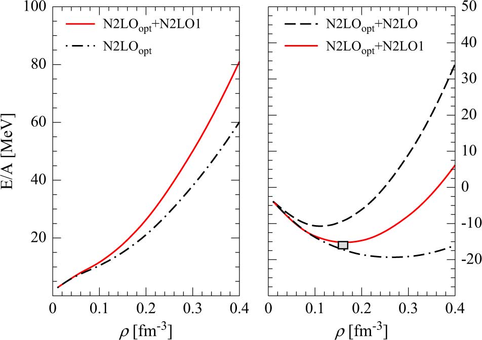
Figure 1. (Colour online) In the figure we show the energy per particle of pure neutron matter (left panel) and SNM (right panel) as function of the nuclear density (ρ) for the two models described in the text. The empirical saturation point of nuclear matter ρ 0 = 0.16 ± 0.01 fm−3,  $E/A{|_{{\rho _0}}} = - 16.0 \pm 1.0 {\rm{MeV}}$ is represented by the grey box in the right panel. See text for details.
The energy per particle of asymmetric nuclear matter, which is essential to describe neutron stars, can be calculated with very good accuracy using the so-called parabolic approximation (Bombaci & Lombardo Reference Bombaci and Lombardo1991):
 $$\frac{E}{A}(\rho ,\beta ) = \frac{E}{A}(\rho ,0) + {E_{{\rm{sym}}}}(\rho ){\beta ^2}{\kern 1pt} ,$$
where E sym(ρ) is the nuclear symmetry energy (Li et al. Reference Li, Ramos, Verde and Vidaña2014) and β is the asymmetry parameter defined in the previous section. Using equation (13), the symmetry energy can be obtained from the difference between the energy per particle of PNM (β = 1) and SNM (β = 0). In Figure 2 we report the plot the density behaviour of E sym.
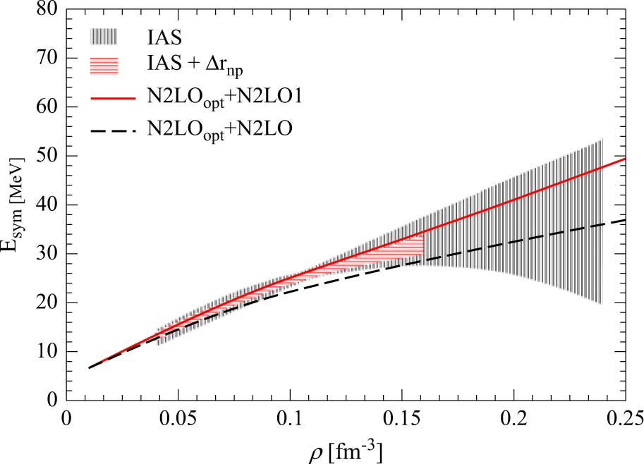
Figure 2. (Colour online) The nuclear symmetry energy is shown as a function of the nucleonic density for the two interaction models used in the present work. The constraints on the symmetry energy obtained by (Danielewicz & Lee (Reference Danielewicz and Lee2014)) using the excitation energies of isobaric analogue states (IAS) in nuclei are represented by the black-dashed band, labelled IAS. The smaller region covered by the red-dashed band labelled IAS+Δrnp (Roca-Maza et al. (Reference Roca-Maza2013)) are additional constraints provided by the data analysis of neutron skin thickness (Δrnp) of heavy nuclei.
In Table 2 we show the values of the symmetry energy and the so-called slope parameter L defined as
 $$L = 3{\rho _0}\frac{{\partial {E_{{\rm{sym}}}}(\rho )}}{{\partial \rho }}{|_{{\rho _0}}}$$
at the calculated saturation density ρ 0 (second column in Table 2) for the two interaction models considered in the present paper. We note that the values of E sym(ρ 0) and L calculated with model N2LOopt+N2LO1 are in a good agreement with those obtained by other calculations based on the BHF approach including two- and three-body forces (see, e.g. Li et al. (Reference Li, Lombardo, Schulze, Zuo, Chen and Ma2006) and Li & Schulze (Reference Li and Schulze2008)) and with the values derived from different experimental data as discussed by Lattimer (Reference Lattimer2014). Our second model instead underestimates both the values of E sym and L.
The incompressibility K ∞ of SNM calculated at saturation density is given by
 $${K_\infty } = 9\rho _0^2\frac{{{\partial ^2}E/A}}{{\partial {\rho ^2}}}{|_{{\rho _0}}}.$$
The value of the incompressibility K ∞ can be obtained analysing experimental data of giant monopole resonance (GMR) energies in medium and heavy nuclei. Such analysis performed first by Blaizot, Gogny, & Grammaticos (Reference Blaizot, Gogny and Grammaticos1976) provided the value K ∞ = 210 ± 30 MeV. The refined analysis of Shlomo, Kolomietz, & Colò (Reference Shlomo, Kolomietz and Colò2006) gave instead the value K ∞ = 240 ± 20 MeV. Recently Stone et al. (2010) on the basis of a re-analysis of GMR data found 250 MeV < K ∞ < 315 MeV. In the last column of Table 2 we have reported the incompressibility K ∞ at the calculated saturation point ρ 0 for the two models considered in the present work. Model N2LOopt + N2LO1 is in very good agreement with the value of K ∞ predicted by Blaizot et al. (Reference Blaizot, Gogny and Grammaticos1976) and Shlomo et al. (Reference Shlomo, Kolomietz and Colò2006). It should be noted that the value of K ∞ is a very important quantity not only for nuclear physics but also for astrophysics. It has been shown indeed that K ∞ is strongly correlated to the physics of supernova explosions and neutron star mergers.
Another important constraint that should be fulfilled by a good nuclear matter EOS concerns the behaviour of the pressure of SNM as function of the nucleonic density. Such constraints are provided by experiments of collisions between heavy nuclei. In such experiments matter is compressed up to ∼4ρ 0, and it is therefore possible to extract important information about the behaviour of the EOS at densities larger than normal saturation density (ρ 0 = 0.16 fm−3)).
The black hatched area in Figure 3 is the region in the pressure–density plane for SNM determined by Danielewicz, Lacey, & Lynch (Reference Danielewicz, Lacey and Lynch2002), performing several numerical simulations able to reproduce the measured elliptic flow of matter in the collision experiments between heavy nuclei.
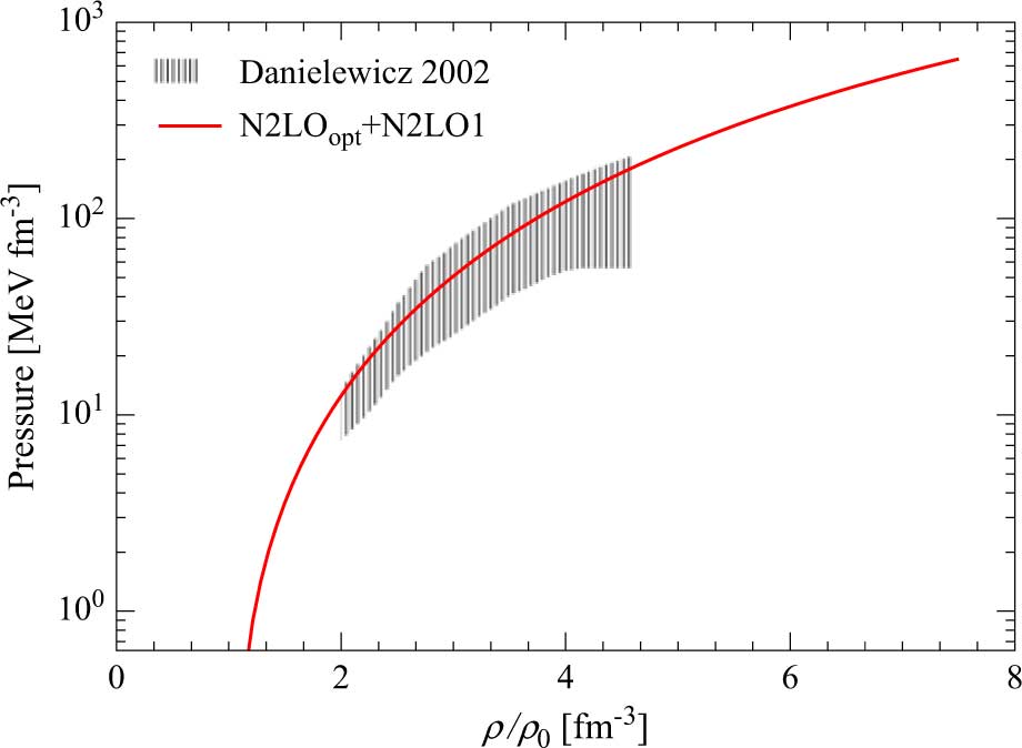
Figure 3. (Colour online) Pressure of SNM as a function of the nucleonic density ρ (in units of the empirical saturation density ρ0 = 0.16 fm−3) for the model N2LOopt + N2LO1. The black hatched area represents the region for SNM which is consistent with the constraints provided by collision experiments between heavy nuclei (Danielewicz et al. Reference Danielewicz, Lacey and Lynch2002).
In the same figure, we show the pressure of SNM for the N2LOopt + N2LO1 (red continuous line) model obtained from the calculated energy per nucleon and using the standard thermodynamical relation:
 $$P(\rho ) = {\rho ^2}\frac{{\partial (E/A)}}{{\partial \rho }}{|_A}.$$
Our results are fully consistent with the empirical constraints given by Danielewicz et al. (Reference Danielewicz, Lacey and Lynch2002).
5. Neutron star structure
We next apply the model N2LOopt + N2LO1, which reproduces various empirical nuclear matter properties at the saturation density (Table 2), to calculate the structure of neutron stars.
The composition of the inner core of neutron stars cannot be completely determined by data from observations and therefore different scenarios are currently under consideration. The appearance of hyperons (Glendenning Reference Glendenning1985; Vidaña et al. Reference Vidaña, Logoteta, Providência, Polls and Bombaci2011) or the transition to a phase with deconfined quarks (quark matter) (Glendenning Reference Glendenning1996; Bombaci et al. Reference Bombaci, Logoteta, Panda, Providência and Vidaña2009; Logoteta et al. Reference Logoteta, Bombaci, Providência and Vidaña2012a; Bombaci & Logoteta Reference Bombaci and Logoteta2013; Logoteta, ProvidŒncia & Vidaña Reference Logoteta, Providência and Vidaña2013) are among the most admissible possibilities.
In this work we want mainly to concentrate on the simplest case of pure nucleonic matter with the aim to establish if the modern chiral nuclear interactions considered here can provide an EOS which is able to fulfil the constraints put by observational data on neutron stars properties. This first check represents a mandatory step before to explore more sophisticated possibilities with additional feasible degrees of freedom. We point out, however, that allowing for a quark deconfinement phase transition and considering the possible existence of a second branch of compact stars (quark stars) with ‘large’ masses compatible with present mass measurements, i.e. within the so-called two families scenario (Berezhiani et al. Reference Berezhiani, Bombaci, Drago, Frontera and Lavagno2003; Bombaci, Parenti & Vidaña Reference Bombaci, Parenti and Vidaña2004, Reference Bombaci, Logoteta, Vidaña and Providência2016; Drago et al. Reference Drago, Lavagno, Pagliara and Pigato2016), is not necessary that the neutron star branch reproduces the limit of two solar masses.
We also report a calculation of the EOS that includes, in addition to nucleons, hyperonic degrees of freedom and in particular the presence of Λ and Σ− hyperons. These are in fact the first hyperon species expected to appear in microscopic calculations of neutron star matter (Glendenning Reference Glendenning1985; Vidaña et al. Reference Vidaña, Logoteta, Providência, Polls and Bombaci2011; Schulze et al. Reference Schulze, Polls, Ramos and Vidaña2006). We thus consider also the so-called hyperonic stars.
In order to determine the mass–radius (M(R)) and mass–central density (M(ρc)) relations for non-rotating neutron stars, one needs first to calculate the β-stable EOS of the system. The composition of β-stable stellar matter is determined by the relations between the chemical potentials of the various constituent species. In this paper we consider neutrino-free matter ( ${\mu _{{\nu _e}}} = {\mu _{{{\bar \nu }_e}}} = {\mu _{{\nu _\mu }}} = {\mu _{{{\bar \nu }_\mu }}}$) in the general case of matter if matter with hyperons. We have
 $${\mu _n} - {\mu _p} = {\mu _{{e^ - }}},\;\;\;\;\;\;\;{\mu _{{e^ - }}} = {\mu _{{\mu ^ - }}},$$
 $${\mu _\Lambda } = {\mu _n},\;\;\;\;\;\;\;{\mu _{{\Sigma ^ - }}} = {\mu _n} + {\mu _{{e^ - }}}.$$
In equations (17) and (18) μn, μp, μ Λ,  ${\mu _{{\Sigma ^ - }}}$, ${\mu _{{e^ - }}}$, and ${\mu _{{\mu ^ - }}}$ are chemical potentials of neutron, proton, Λ, Σ−, electron, and muon. Finally charge neutrality requires
 $${\rho _p} = {\rho _{{\Sigma ^ - }}} + {\rho _{{e^ - }}} + {\rho _{{\mu ^ - }}}.$$
The various chemical potentials of baryons (B = n, p, Λ, Σ−) and leptons (l = e −, μ −) are determined through
 $${\mu _{\rm{B}}} = \frac{{\partial \varepsilon }}{{\partial {\rho _{\rm{B}}}}},\;\;\;\;{\mu _{\rm{l}}} = \frac{{\partial \varepsilon }}{{\partial {\rho _{\rm{l}}}}},$$
where ɛ = ɛ N + ɛY + ɛ L is the total energy density which sums up the nucleonic contribution ɛ N, the hyperonic one ɛY, and the leptonic one ɛ L. The nucleonic contribution ɛ N has been calculated using the N2LOopt + N2LO1 nuclear interaction and the thermodynamical relation ɛ N = ρE/A(ρ,β), with the energy per particle E/A(ρ, β) of asymmetric nuclear matter calculated in BHF approximation and employing the parabolic approximation (Bombaci & Lombardo Reference Bombaci and Lombardo1991). For the hyperonic contribution ɛY we have used the parametric form of the BHF energy per particle of asymmetric hyperonic matter provided by Rijken & Schulze (Reference Rijken and Shulze2016) and obtained using the nucleon–hyperon (NY) and hyperon–hyperon (YY) interactions. More specifically Rijken & Schulze (Reference Rijken and Shulze2016) used the NY Nijmegen soft core NSC08b potential (Rijken, Nagels & Yamamoto Reference Rijken, Nagels and Yamamoto2010) supplemented with the new YY Nijmegen soft core NSC08c potential (Nagels, Rijken & Yamamoto Reference Nagels, Rijken and Yamamoto2014). We note that these interactions have been derived following the scheme of traditional meson exchange theory and not in the framework of ChPT. However, they provide an accurate description of the available hypernuclear data (Rijken et al. Reference Rijken, Nagels and Yamamoto2010).
We have then self-consistently solved the equations (17), (18), (19), and (20) as function of the total baryonic density  $\rho = {\rho _n} + {\rho _p} + {\rho _\Lambda } + {\rho _{{\Sigma ^ - }}}$ and obtained the EOS for β-stable hyperonic matter with nucleons, hyperons, electrons, and muons (μ −).
The composition of β-stable nucleonic matter is shown by the continuous lines in Figure 4. The black circle on the black line, which represents the proton fraction, marks the density threshold for the direct URCA processes  $n \to p + {e^ - } + {\bar \nu _e}$, p + e − → n + ve (Lattimer et al. Reference Lattimer, Pethick, Prakash and Haensel1991). In our model this threshold is ρDU = 0.339 fm−3 which corresponds to a neutron star mass M(ρDU) = 0.97 M⊙. The dashed lines in Figure 4 represent the results of the solution of the β-equilibrium equations for hyperonic matter with Λ and Σ− hyperons. The Λ hyperon is the first hyperonic species to appear at a density around 0.37 fm−3 while the Σ− hyperon appears at density of 0.47 fm−3. This behaviour is a new feature of modern NY interactions which find a much more repulsive contribution in the NΣ− channel to the total energy density. The same trend has been also found by recent NY interactions derived in ChPT by Haidenbauer & Meißner (Reference Haidenbauer and Meißner2015). Such a repulsion leads to the appearance of the Λ hyperon before the Σ− one contrarily to the predictions of older NY interaction models (Schulze et al. Reference Schulze, Polls, Ramos and Vidaña2006).
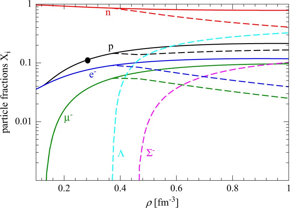
Figure 4. (Colour online) Particle fractions in β-stable neutron star matter for model N2LOopt + N2LO1. The continuous lines (dashed lines) refer to particle fractions in the case of β-stable nucleonic matter (hyperonic matter).
In order to calculate the neutron stars structure, we have numerically solved the equations for hydrostatic equilibrium in general relativity (Tolman Reference Tolman1939; Oppenheimer & Volkoff Reference Oppenheimer and Volkoff1939). For nucleonic density smaller than 0.08 fm−3 we have matched our EOS models of the core with the Negele & Vautherin (Reference Negele and Vautherin1973) and Baym, Pethick, & Sutherland (Reference Baym, Pethick and Sutherland1971) EOSs which model neutron stars crust.
In Figure 5 we show the results of our calculations. In the left (right) panel we plot the mass–radius (mass–central density) relations for our models. Referring now to the left panel in Figure 5, the hatched regions are constraints derived from the analysis of observational data of both transiently accreting and bursting X-ray sources obtained by Steiner et al. (Reference Steiner2010); Steiner, Lattimer, & Brown (Reference Steiner, Lattimer and Brown2013). We note the maximum mass M max = 1.99 M⊙ obtained for nucleonic stars, i.e. for the EOS model including only nucleons (continuous line in Figure 5), is compatible with present neutron star mass measurements and in particular with the measured mass 2.01 ± 0.04 M⊙ (Antoniadis et al. Reference Antoniadis2013) of the neutron star in PSR J0348+0432 (strip with boundaries marked with blue lines in Figure 5). In addition, our results are also in rather good agreement with the empirical constraints on the mass–radius relationship reported in Steiner et al. (Reference Steiner2010); Steiner et al. (Reference Steiner, Lattimer and Brown2013). We note, however, that presently there is no general agreement on neutron star radii measurements due to the large uncertainties in the techniques used to extract this quantity. For instance, small stellar radii in the range of 9–12 km (Guillot et al. Reference Guillot, Servillat, Webb and Rutledge2013) have found considering information from spectral analysis of X-ray emission from quiescent X-ray transients in low-mass binaries (QLMXBs). Larger radii around 16 km are instead obtained considering data on neutron stars with recurring powerful bursts. However, these last measurements are subject to large uncertainties (Poutanen et al. Reference Poutanen2014). In a recent work Lattimer & Prakash (Reference Lattimer and Prakash2016) suggests that neutron star radii should lie in the range between 10.7 and 13.1 km.
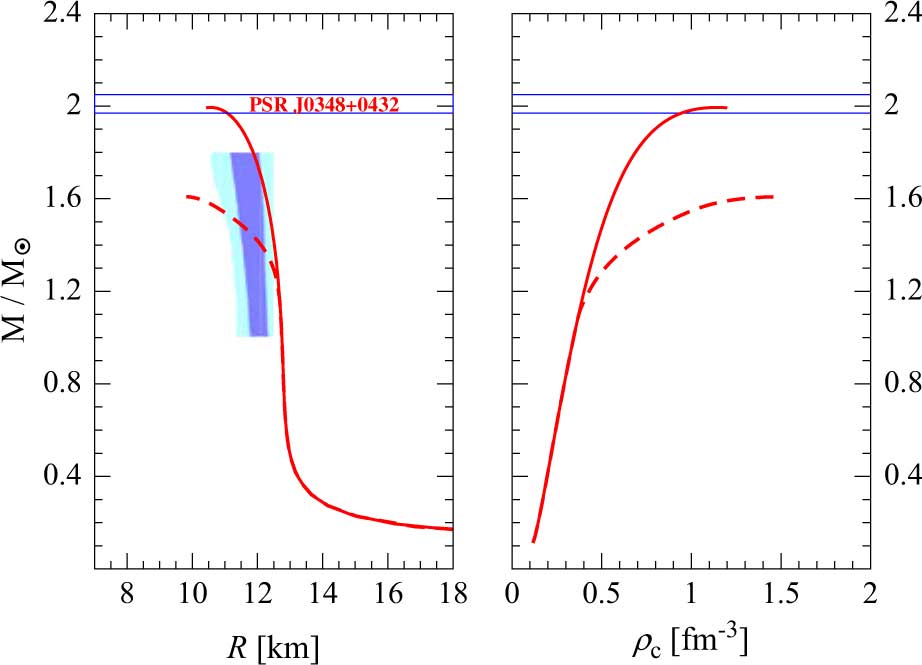
Figure 5. (Colour online) Mass–radius (M(R)) (left panel) and mass–central density (M(ρc)) (right panel) relationships for the models described in the text. The continuous lines refer to the calculation performed considering the EOS containing only nucleonic degrees of freedom, while the dashed lines have been obtained including also the Λ and the Σ− hyperons in the calculation. The hatched region in the left panel represents the mass–radius constraints obtained by Steiner et al. (Reference Steiner2010, Reference Steiner, Lattimer and Brown2013). The strip with boundaries marked with blue lines stands for the measured mass 2.01 ± 0.04 M⊙ (Antoniadis et al. Reference Antoniadis2013) of the neutron stars in PSR J0348+0432.
The red dashed lines in Figure 5 represent the mass–radius (left panel) and mass–central density (right panel) relations for hyperonic stars (i.e. for the EOS model including hyperons in addition to nucleons). In this case there is a sizable decrease of the stellar maximum mass down to M max = 1.6 M⊙, a value which is incompatible with measured neutron star masses. This outcome is caused by the softening of the EOS due to the presence of hyperons in the stellar core (Schulze et al. Reference Schulze, Polls, Ramos and Vidaña2006; Vidaña et al. Reference Vidaña, Logoteta, Providência, Polls and Bombaci2011; Logoteta et al. Reference Logoteta, Bombaci, Providência and Vidaña2012b).
This difficulty to reconcile the measured masses of neutron stars with the seemingly unavoidable presence of hyperons in their interiors is called hyperon puzzle (Lonardoni et al. Reference Lonardoni, Lovato, Gandolfi and Pederiva2015; Bombaci Reference Bombaci2017; Chatterjee & Vidaña Reference Chatterjee and Vidaña2016) in neutron stars. This unsolved puzzle is currently the subject of several investigations, and various possible solutions have been proposed. Some researches pointed out the importance of taking into account the effect of hyperonic three-body forces between nucleons and hyperons (Lonardoni et al. Reference Lonardoni, Lovato, Gandolfi and Pederiva2015; Vidaña et al. Reference Vidaña, Logoteta, Providência, Polls and Bombaci2011; Chatterjee & Vidaña Reference Chatterjee and Vidaña2016), while other investigations (Bombaci et al. Reference Bombaci, Logoteta, Vidaña and Providência2016; Drago et al. Reference Drago, Lavagno, Pagliara and Pigato2016) underline the possibility for a phase transition to quark matter at large baryonic density and the existence of a second branch of compact stars (quark stars) with ‘large’ masses compatible with present mass measurements. Finally we emphasise that also the two-body YY interaction can play a role in solving the hyperon puzzle. In fact, as shown by Schulze et al. (Reference Schulze, Polls, Ramos and Vidaña2006), the new NSC08c YY interaction makes the EOS stiffer and allows to increase the maximum mass of about 0.25 M⊙ with respect to the case when only NN and NY interactions are taken into account to describe the two-body baryon–baryon interactions.
The properties of the maximum mass configuration for our models of nucleonic and hyperonic stars are reported in Table 3. These results are in good agreement with other calculations based on microscopic approaches. Concerning this point it is interesting to note that our present findings are very similar to those reported in Taranto, Baldo, & Burgio (Reference Taranto, Baldo and Burgio2013) where nuclear matter properties and β-stable EOS have been obtained using the BHF approach and employing two- and three-body forces based on the meson-exchange theory. In addition, our results are in good accord with those in Bombaci & Logoteta (Reference Bombaci and Logoteta2018) where the neutron stars structure was described adopting chiral potentials calculated in the so-called Δ-full theory both at two- and three-body levels. Such agreement provides an independent way to check the correct behaviour of the interactions used in the present work at large baryonic density. We note indeed that the interactions derived in ChEFT are characterised by a low-momentum expansion and therefore can be trusted up to baryonic densities for which the Fermi momentum is of the order of magnitude of the cut-off set in the regulator function. At larger densities, the EOS should be extrapolated or an accurate analysis of convergence of the many-body calculation has to be properly accounted for. We note that for neutron stars these considerations are mandatory because the maximum density reached in the core can be even larger than 1 fm−3 (see Table 3).
Table 3. Mass (in unit of solar mass M ⊙ = 1.989 × 1033g), corresponding radius (in km) and central density (in fm−3) for the neutron star configuration corresponding to the maximum masses of Figure 5
The gravitational redshift of a signal emitted from the stellar surface is given by
 $${z_{{\rm{s}}urf}} = (1 - \frac{{2GM}}{{{c^2}R}}{)^{ - 1/2}} - 1.$$
The measurements of zsurf of spectral lines can provide a direct information on the neutron star compactness parameter:
 $${x_{GR}} = \frac{{2GM}}{{{c^2}R}}\;$$
and therefore on the EOS of neutron star matter. The calculation of the surface gravitational redshift for our two EOS models is shown in Figure 6. The two horizontal lines in the same figure stand for the measured gravitational redshift z = 0.35 for the X-ray bursts source in the low-mass X-ray binary EXO 07482−676 (Cottam, Paerels, & Mendez Reference Cottam, Paerels and Mendez2002) and  $z = 0.205_{ - 0.003}^{ + 0.006}$ for the isolated neutron star RX J0720.4−3125 (Hambaryan et al. Reference Hambaryan2017).
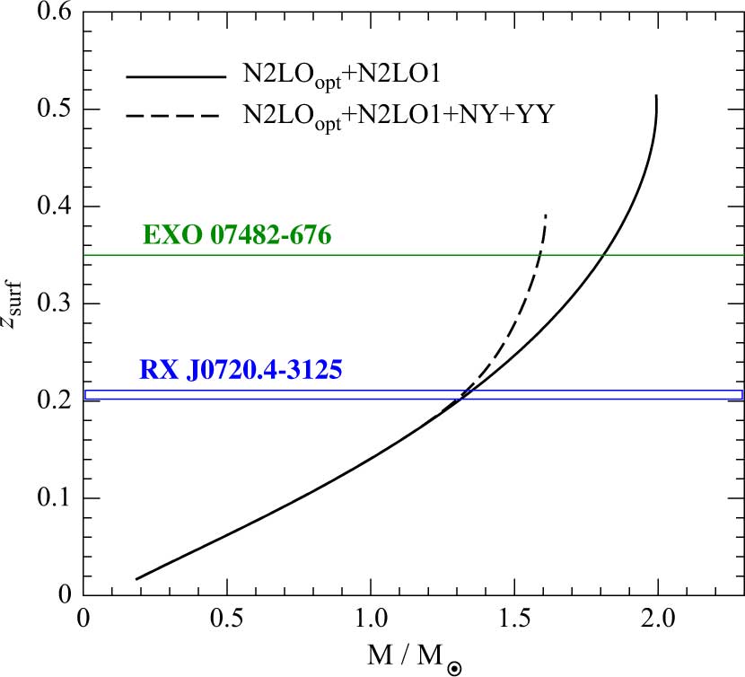
Figure 6. (Colour online) Gravitational redshift calculated at the neutron star surface as a function of the stellar gravitational mass for the two EOS models used in our work. The horizontal lines stand for the measured gravitational redshift z = 0.35 for the X-ray bursts source in the low-mass X-ray binary EXO 07482−676 (Cottam et al. Reference Cottam, Paerels and Mendez2002) and  $z = 0.205_{ - 0.003}^{ + 0.006}$ for the isolated neutron star RX J0720.4−3125 (Hambaryan et al. Reference Hambaryan2017).
6. Summary
We have investigated the behaviour and the properties of β-stable nuclear matter using two microscopic models based on nuclear hamiltonians obtained from ChPT at the N2LO in the framework of many-body BHF approach. In particular, we have used the non-local NN chiral potential derived by Ekström et al. (Reference Ekström, Jansen, Wendt, Hagen, Papenbrock, Bacca, Carlsson and Gazit2014), which is able to reproduce the NN scattering data with a χ 2/datum ∼1. In order to get a good description of nuclear matter at saturation density, we have included in our calculation also a TNF consistently calculated at the same order of ChPT. Concerning the TNF, we have explored two different parametrisations: the first one (N2LO) fitted to reproduce binding energies of light nuclei, while the second one (N2LO1) fitted to reproduce a good saturation point of SNM. We have shown that in the first case it was not possible to reproduce also good properties of nuclear matter at saturation density. For the second case, we have shown that once the saturation point of SNM was well reproduced, other nuclear matter properties at the saturation density were also well determined. We have later calculated the EOS for β-stable nuclear matter for our best model, namely the N2LOopt + N2LO1 one, and determined the neutron stars structure. We have found that the maximum mass obtained is compatible with the present measured neutron star masses. In addition we have found that the mass–radius relation for nucleonic stars is in a quite good agreement with the mass–radius constraints determined by Steiner et al. (Reference Steiner2010); Steiner et al. (Reference Steiner, Lattimer and Brown2013). Finally, we have extended our EOS model to include hyperons and we have thus calculated the corresponding hyperonic star properties. Confirming the results of previous studies, e.g. (Schulze et al. Reference Schulze, Polls, Ramos and Vidaña2006; Vidaña et al. Reference Vidaña, Logoteta, Providência, Polls and Bombaci2011; Lonardoni et al. Reference Lonardoni, Lovato, Gandolfi and Pederiva2015; Chatterjee & Vidaña Reference Chatterjee and Vidaña2016), we have found that the inclusion of hyperons leads to a substantial reduction of the value of the maximum mass which turns out to be not compatible with measured neutron star masses. This so-called hyperon puzzle is one of the hottest topics in neutron star physics which is stimulating copious experimental and theoretical research in hypernuclear physics.
Several extensions of the present model to include hyperonic three-body forces and quark degrees of freedom are indeed under consideration. In addition, the inclusion of thermal effects necessary for application to supernova explosions and consistent neutron star merger simulations are also in development.
Author ORCIDs.
D. Logoteta, http://orcid.org/0000-0003-2011-2328; I. Bombaci, http://orcid.org/0000-0002-0497-7375.
Acknowledgements
This work has been partially supported by ‘NewCompstar’, COST Action MP1304.


