


1. Introduction
Shortly after the original discovery of pulsars (Hewish et al. Reference Hewish, Bell, Pilkington, Scott and Collins1968), the radio emission from pulsars was found to be polarised (Lyne & Smith Reference Lyne and Smith1968). The polarimetric profiles of pulsars provide useful tools to classify and study pulsar geometry (e.g. Rankin Reference Rankin1983; Brinkman et al. Reference Brinkman, Mitra and Rankin2019). Most pulsars tend to show a significant amount of linear polarisation—about 20%, on average, and reaching up to 100% in some cases (e.g. Weltevrede & Johnston Reference Weltevrede and Johnston2008; Han et al. Reference Han, Demorest and Lyne2009). The degree of linear polarisation generally tends to decrease with increasing observing frequency (e.g. Morris et al. Reference Morris, Graham and Sieber1981; von Hoensbroech et al. Reference von Hoensbroech, Kijak and Krawczyk1998). The physical explanation for this is not straightforward, though may be due to higher frequencies traversing more of the magnetosphere (Johnston et al. Reference Johnston, Karastergiou, Mitra and Gupta2008), or the birefringence of plasma in the open field-line region of pulsar magnetospheres (e.g. McKinnon Reference McKinnon1997). Many pulsars also show some circular polarisation—about 10%, on average (e.g. Gould & Lyne Reference Gould and Lyne1998; Weisberg et al. Reference Weisberg1999; Johnston & Kerr Reference Johnston and Kerr2018).
The radio emission from pulsars is broadly thought to originate within the open field lines of the magnetosphere, with the emission beam centred on the magnetic axis (e.g. Komesaroff Reference Komesaroff1970). Consequently, the linear polarisation position angle (PA) will be determined by the direction of the magnetic field line as it sweeps across our line-of-sight. The PA measured as a function of rotational phase, referred to as the PA curve, is generally expected to delineate an S-shape, that is, the PA will vary more slowly at the outer wings of the pulse profile compared to the centre. This is referred to as the rotating vector model (RVM; Radhakrishnan & Cooke Reference Radhakrishnan and Cooke1969). Fitting the RVM model to the observed PAs provides an estimation of the emission beam size and the inclination angle of the magnetic axis with respect to the rotation axis (e.g. Narayan & Vivekanand Reference Narayan and Vivekanand1982; Everett & Weisberg Reference Everett and Weisberg2001).
For some pulsars, especially those with medium or low levels of linear polarisation, their PA curves show interruptions of approximately 90°, referred to as orthogonal jumps (e.g. McKinnon & Stinebring Reference McKinnon and Stinebring1998). For example, Karastergiou et al. (Reference Karastergiou, Roberts, Johnston, Lee, Weltevrede and Kramer2011) present the polarimetric profiles for PSR J0738–4042 at different epochs and find that the presence of orthogonal jumps in the PA curves is associated with reduced degrees of linear polarisation. Such observational evidence affirms the concept that pulsar emission could comprise two superposed orthogonal polarisation modes (OPMs; e.g. McKinnon & Stinebring Reference McKinnon and Stinebring2000). There have been a number of associated studies from both observational (e.g. Edwards & Stappers Reference Edwards and Stappers2004; Noutsos et al. Reference Noutsos2015) and theoretical (e.g. Gangadhara Reference Gangadhara1997; Melrose et al. Reference Melrose, Miller, Karastergiou and Luo2006; van Straten & Tiburzi Reference van Straten and Tiburzi2017) points of view. However, the nature of the OPMs is still one of the least understood aspects of pulsar emission.
Of the >2 600 known pulsarsFootnote a (Manchester et al. Reference Manchester, Hobbs, Teoh and Hobbs2005), only around one-third have polarimetric properties currently available, and this is mostly limited to ˜1.4 GHz frequencies. Extensive polarimetric studies have been published by Gould & Lyne (Reference Gould and Lyne1998) using the Lovell telescope, Weisberg et al. (Reference Weisberg1999) using the Arecibo telescope, and Manchester et al. (Reference Manchester, Han and Qiao1998) and Johnston & Kerr (Reference Johnston and Kerr2018) using the Parkes telescope. There have been a limited number of such investigations at frequencies below ˜1GHz. Some studies have been conducted using the Giant Metrewave Radio Telescope (GMRT; Swarup et al. Reference Swarup, Ananthakrishnan, Kapahi, Rao, Subrahmanya and Kulkarni1991; Roy et al. Reference Roy, Gupta, Pen, Peterson, Kudale and Kodilkar2010), including the Meterwavelength Single-pulse Polarimetric Emission Survey at 333 and 618 MHz (Mitra et al. Reference Mitra, Basu, Maciesiak, Skrzypczak, Melikidze, Szary and Krzeszowski2016). At lower radio frequencies, Noutsos et al. (2015) undertook polarimetric studies below 200 MHz using the Low-Frequency Array (LOFAR; van Haarlem et al. Reference van Straten2013; Stappers et al. Reference Stappers2011), for pulsars observable from the northern hemisphere. For southern pulsars, the Murchison Widefield Array (MWA; Tingay et al. Reference Tingay2013; Wayth et al. Reference Wayth2018) provides an excellent opportunity for polarimetric studies of pulsars at frequencies below ˜300 MHz. Low-frequency polarisation observations of pulsars provide precise probes of the magneto-ionic ISM; for example, towards reconstructing the structure of the Galactic magnetic field (Han et al. Reference Han, Demorest and Lyne2009; Sobey et al. Reference Sobey2019). Furthermore, detailed studies of low-frequency polarimetric profiles, in combination with higher frequency data, can provide further insights into the pulse profile evolution and potentially help elucidate the magnetospheric radio emission mechanism. They also serve as a useful reference for future pulsar studies planned with the Square Kilometre Array (SKA).
Traditionally, polarimetric studies were mostly performed using large single dish antennas or interferometer telescopes comprised of parabolic dishes. For single dish telescopes like Parkes, polarimetric calibration is achieved by comparing an observed full-Stokes pulse profile to a standard profile template (e.g. using long-term monitoring of PSR J0437–4715). This allows the complex Jones matrix, which describes the transfer function of the signal through the system, to be determined (e.g. Hamaker et al. Reference Hamaker, Bregman and Sault1996; Heiles et al. Reference Heiles2001; Johnston Reference Johnston2002; van Straten Reference van Haarlem2013). For interferometers like the Westerbork Synthesis Radio Telescope (WSRT) or GMRT, the procedure for forming a tied-array beam is to add the voltages of all telescopes after correcting their relative phases. This means that the tied-array signal can be calibrated by determining an overall system Jones matrix, and thus the polarisation calibration process is similar to that of single dishes (e.g. Edwards & Stappers Reference Edwards and Stappers2004; Mitra et al. Reference Mitra, Basu, Maciesiak, Skrzypczak, Melikidze, Szary and Krzeszowski2016).
For low-frequency aperture-array instruments such as LOFAR, the MWA, and the upcoming SKA-Low (i.e. the low-frequency component of the SKA), the approach is quite different. Since the arrays have no moving parts, tile/station beam pointings are formed by electronic manipulation of the dipole signals using analogue/digital beamformers (Tingay et al. Reference Tingay2013; van Haarlem et al. Reference van Straten2013). This beam response is strongly dependent on the pointing direction and frequency (e.g. Noutsos et al. Reference Noutsos2015) and is more difficult to model compared to that for a single dish. Accurate calibration of the full polarimetric response is necessary for aperture arrays to facilitate reliable polarisation studies. This procedure is fairly complex, due to a number of factors: the wide field of view; multiple receiving elements; frequency-dependent beam shape; the absence of an injected artificial calibration signal; and the modulation of calibration errors by the time-variable ionosphere. Thus, developing a suitable calibration/beamformation strategy for the MWA and verifying that it is satisfactorily robust and reliable is an essential prerequisite for performing any polarimetric pulsar work with these new generation radio arrays.
In Paper 1 of this series, we described the algorithms and pipeline that we have developed to form the tied-array beam products from the summation of calibrated signals of the antenna elements (Ord et al. submitted). In this paper, we present the first polarimetric study of two bright southern pulsars, PSRs J0742– 2822 and J1752–2806, at frequencies below 300 MHz. Our primary goal is to investigate their polarimetric properties as a function of frequency and to ascertain the reliability of the MWA’s polarimetric performance. We describe our observations and data processing methods in Section 2. In Section 3 we summarise the optimal calibration strategy and reproducibility of the polarimetric profiles. In Section 4 we describe how we measure the Faraday rotation and use it to estimate the instrumental leakage. We describe the polarimetric properties of the two pulsars and compare our profiles with published polarimetric profiles at higher frequencies, in Section 5. In Section 6, we discuss our results, and a summary of our work is given in Section 7.
2. Observations and data processing
Our observations were taken with the Phase I MWA, where the array was comprised of 128 tiles—each tile consists of 16 dual-polarisation dipole antennas arranged in a regular 4 × 4 grid, operating at 80–300 MHz. The development of the Voltage Capture System (VCS; Tremblay et al. Reference Tremblay2015) extended the capabilities of the MWA from an imaging interferometer, allowing it to record high-time and high-frequency resolution voltage data and enabling time-domain astrophysics. This allows the MWA to provide phase-resolved observations of pulsars (e.g. Bhat et al. Reference Bhat2018).
We use multiple observations of two bright polarised pulsars that pass through the zenith at the MWA site, PSRs J0742–2822 and J1752–2806, to empirically examine the MWA’s polarimetric response in the beamforming (tied-array) mode, and its stability across the dipole/antenna beam. Here, we describe the properties of target pulsars, our observing strategy, calibration, beamformation, data reduction procedures, as well as archival MWA observations used for our comparison studies.
2.1. Target pulsars
PSR J0742–2822 has a period (P) of 167 ms and a dispersion measure (DM; the integrated electron column density along the line-of-sight) of 73.73 cm−3 pc. It is highly polarised with a linear polarisation degree of around 70% and a flux density of ˜300 mJy at 400 MHz (Lorimer et al. Reference Lorimer, Yates, Lyne and Gould1995; Gould & Lyne Reference Gould and Lyne1998; Mitra et al. Reference Mitra, Basu, Maciesiak, Skrzypczak, Melikidze, Szary and Krzeszowski2016), and hence a linear polarisation flux density of ˜200 mJy at 400 MHz.
We note that PSR J0742–2822 is known to exhibit emission mode changing; however, the timescale is relatively long, typically ˜95 days (Keith et al. Reference Keith, Shannon and Johnston2013). All of our observations of PSR J0742– 2822 were taken during the same night within 5 h (see below) and, therefore, it is likely that all of our data were taken when the pulsar was in the same emission mode. This is consistent with our results (see Section 3.2).
PSR J1752–2806 (P = 563 ms, DM = 50.37 cm−3 pc) is a moderately polarised pulsar with a linear polarisation degree of around 10% and a flux density of ˜1100 mJy at 400 MHz (Lorimer et al. Reference Lorimer, Yates, Lyne and Gould1995; Gould & Lyne Reference Gould and Lyne1998; Mitra et al. Reference Mitra, Basu, Maciesiak, Skrzypczak, Melikidze, Szary and Krzeszowski2016); thus, its linear polarisation flux density is ˜110 mJy at 400 MHz. Typically, flux densities of pulsars follow a power-law with a spectral index of about −1.6, and so we expect pulsars to be around three times brighter at 200 MHz.
2.2. Observing strategy
For each pulsar, we obtained and compared the polarimetric pulse profiles over a range of zenith angles (ZA) across a wide range of observing frequencies. These data allowed us to assess the quality, reliability, and repeatability of our calibration and beamformation process.
Three specific elements of the data were used to investigate the effect on the polarimetric profiles produced, namely:
• sky position of the target pulsar;
• sky position of the calibrator source; and
• calibration strategy, that is, observing a calibrator source prior to the target versus in-field calibration.
Consequently, the observing strategy that we adopted is as follows. For each of the two target pulsars, we recorded five short observations of 5 min each, separated by roughly 1 h, with the middle observation pointing towards the zenith and the others towards ZA up to 30°, as shown in Figure 1. The five observations for each pulsar are labelled P1–P5, in the order of the observing start times. We also recorded a 5-min dedicated calibrator observation before each pulsar observation. Thus, there are also five dedicated calibrator observations in total for each pulsar. Similarly, they are named C1–C5, in the order of their observing start times (see Figure 1). The pointing information for the observations is summarised in Table 1.
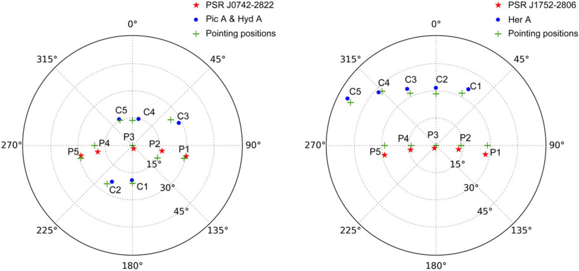
Figure 1. (Left) Locations and MWA pointing directions for PSR J0742–2822 and its calibrators Pictor A (C1, C2) and Hydra A (C3–C5). (Right) Locations and MWA pointing directions for PSR J1752–2806 and its calibrator Hercules A. For both panels, the azimuth angles and ZA are shown in horizontal coordinates, azimuth = 0° represents North and azimuth=90° represents East. Red stars indicate the position of pulsars (labelled P1–P5 in order of observation start time); blue circles indicate the position of calibrators (labelled C1–C5 in order of observation start time); green crosses indicate the pointing centre for each observation. Since the MWA points towards ‘sweet’ spots in the sky (dictated by the analogue beamformer settings), there is usually some offset between the pointing centre direction and the position of the target.
Table 1. Observing parameters for PSR J0742–2822, PSR J1752–2806, and calibrator sources.
The VCS records data after the second stage of channelisation in the MWA signal path, with a 10 kHz frequency resolution and a 100 μs time resolution. Data from our observations were recorded at frequencies spread across the entire MWA band, from 76.80 to 312.32 MHz, in 24 coarse (1.28 MHz-wide) channels (see Table 2). These non-contiguous coarse channels were recorded simultaneously, each split into 128 fine (10 kHz-wide) channels.
Table 2. Summary of the centre observing frequencies, f.
The dispersion delay at each frequency for PSRs J0742–2822 and J1752–2806 is presented in milliseconds (Δt) and per cent of the pulse period (ΔP).
2.3. Calibration
In order to coherently sum the signals from the MWA tiles, we need to calibrate the array to determine the direction-independent complex gains (amplitudes and phases) for each tile first. The Real Time System (RTS; Mitchell et al. Reference Mitchell, Greenhill, Wayth, Sault, Lonsdale, Cappallo, Morales and Ord2008) was used for this calibration process. The RTS generated solutions for each tile at each frequency band from calibrator observation. This process utilised the MWA’s analytical beam model. A more detailed description of the calibration process can be found in Section 2.4 of Paper 1.
Each dipole antenna in the MWA array has a beam response, which effectively ‘point’ towards the zenith, and each tile (comprising 4 × 4 dipoles) has analogue beamformers that add delays to the signals to steer the ‘tile beam’ towards the target source. We can coherently sum the signals from all 128 tiles to form a tied-array beam. In this sense, all of our calibrations can be considered as ‘off-axis’.
For the verification described in this paper, we used both the dedicated calibrator observations (as described in Section 2.2) and in-field calibration. For in-field (self) calibration, we processed the complex voltage data from the pulsar observations using an offline version of the MWA correlator (Ord et al. Reference Ord2015) to generate visibilities in the same format as the dedicated calibrator observations.
2.4. Beamforming
A detailed description of the beamforming process is presented in Paper 1. Here, we briefly summarise the process. We used the calibration solutions to coherently combine the signals from all 128 tiles to form a tied-array (phased array) beam towards the target pulsar by applying phase rotations to correct for geometric delays between the tiles so that the entire array ‘points’ towards the target position. This procedure involves applying direction-independent phase and amplitude corrections from the calibration solutions to the signals received by each tile. Meanwhile, since the calibration solution is direction independent, we rotate the calibration solution towards the target position according to the analytic tile beam model (the same as that used in the RTS calibration process) to retrieve the direction-dependent complex gain components before we apply it in the beamforming operation.
2.5. Data reduction and analysis
The beamforming pipeline writes out the data in the PSRFITS format (Hotan et al. Reference Hotan, van Straten and Manchester2004). These data were then incoherently de-dispersed and folded using DSPSRFootnote b (van Straten & Bailes Reference van Straten and Bailes2011) and the timing ephemeris from the pulsar catalogue1 (Manchester et al. Reference Manchester, Hobbs, Teoh and Hobbs2005). For further analysis we mostly used the PSRCHIVEFootnote c software (Hotan et al. Reference Hotan, van Straten and Manchester2004; van Straten et al. Reference van Straten, Demorest and Oslowski2012). The optimal DM (maximising the signal-to-noise ratio in the total intensity pulse profile) was found using the PSRCHIVE pdmp routine. The total degree of linear polarisation is estimated as equivalent integrated on-pulse flux of the linearly polarised profileFootnote d. This is essentially the continuum equivalent quantities as it is estimated from the integrated on-pulse profile.
To obtain the polarimetric profiles for the pulsars and estimate the degree of linear polarisation, we need to correct for the effect of Faraday rotation. We determined the Faraday rotation measure (RM, in units of rad m−2) towards the pulsars using the technique of RM Synthesis (Burn Reference Burn1966; Brentjens & de Bruyn Reference Brentjens and de Bruyn2005). We used the pre-processing parts of the rmfit quadratic fitting function within the PSRCHIVE package (Noutsos et al. Reference Noutsos, Johnston, Kramer and Karastergiou2008) to extract the Stokes I, Q, U, V parameters (as a function of frequency) from the peak of the average total intensity pulse profile. The Stokes parameters were used as an input to the RM Synthesis code written in pythonFootnote e. We also used the associated RM-CLEAN4 method (Heald et al. Reference Heald, Braun and Edmonds2009; Michilli et al. Reference Michilli2018) to determine the fraction of instrumental polarisation leakage near 0 rad m−2. We obtained the dirty and RM-CLEAN-ed Faraday spectra (or Faraday dispersion functions) output for each pulsar observation. The RM was recorded as the location of the peak in the clean Faraday spectrum.
The ionosphere imparts additional Faraday rotation, RMion, to the total observed RM, RMobs. The ionospheric contribution must be subtracted in order to obtain the RM due to the interstellar medium (ISM) alone, that is, RMISM = RMobs – RMion. The RMion is both time and direction dependent and was estimated towards each target source line-of-sight (at the corresponding ionospheric pierce point) for the average time of each observation. To estimate RMion, we employed an updated version of ionFRFootnote f (Sotomayor-Beltran et al. Reference Sotomayor-Beltran2013) using input data from the latest version of the International Geomagnetic Reference FieldFootnote g (IGRF-12; Thébault et al. Reference Thébault2015) and the International Global Navigation Satellite Systems Service (IGS) vertical total electron content (TEC) mapsFootnote h (e.g. Hernández-Pajares et al. Reference Hernández-Pajares2009) for each observation date. Using the Long Wavelength Array, Malins et al. (Reference Malins, White, Taylor, Stovall and Dowell2018) find that local high-cadence TEC measurements are superior to the global TEC models for ionospheric RM correction. However, the difference between the local measurements and the global models is not significant for our range of observing frequencies.
2.6. Archival VCS data
In addition to multiple short observations using non-contiguous frequency channels, we also make use of archival VCS data for PSR J1752–2805 for comparison. Specifically, here we present results from a 40-min zenith-pointing observation from June 2015 (observation ID: 1117643248), over a contiguous 30.72 MHz bandwidth at a central frequency of 118.40 MHz. We used an observation of a calibrator source, 3C444, taken 6 h later that night (observation ID: 1117643248, with azimuth = 288.43 deg, ZA = 22.02 deg) to calibrate and beamform the data using the same procedure as described above.
3. Verification of the polarimetric response
Theoretically, the polarimetric response including leakage for the array can be estimated using the MWA beam models and the intrinsic cross-polarisation ratio (IXR) (Carozzi & Woan Reference Carozzi and Woan2011). In practice, it is difficult to estimate this accurately due to the discrepancy between the actual beam response and our beam models. Although significant efforts have been made to improve our understanding of the MWA’s actual beam response (e.g. Sutinjo et al. Reference Sutinjo, O’Sullivan, Lenc, Wayth, Padhi, Hall and Tingay2015; Sokolowski et al. Reference Sokolowski2017; Line et al. Reference Line2018), it is still an ongoing area of research. Any discrepancy between the actual beam performance and the assumed beam model will manifest as errors in the polarimetric response that are a function of pointing direction. As described in Paper 1, the current MWA tied-array data processing (calibration and beamforming) still uses a simple analytical beam model. Here, we estimate the polarisation leakage empirically by comparing the results from each target pulsar at different sky coordinates (Az, ZA) calibrated with solutions from multiple (Az, ZA). Through this comparison, we first determine the optimal calibration strategy (Section 3.1), and then estimate the reproducibility of the polarimetric profiles for the two target pulsars (Section 3.2). Given the large range of instrumental polarisation exhibited by a phased array as a function of pointing, any small errors in the calibration process will manifest as large errors in measured polarisation. We therefore use the reproducibility of the pulsar polarimetric profile over a wide range of instrumental polarisation as a proxy for calibratibility.
3.1. Determining the optimal calibration strategy
In order to determine the optimal calibration strategy, different calibration solutions were used to beamform multiple pointings for both pulsars. For PSR J0742−2822, the in-field calibration and five dedicated calibrations are compared for each of the five short pulsar observations. However, for PSR J1752−2806, we were unable to benefit from in-field calibration because its line-of-sight is closer to that of the Galactic centre (l = 1.54°, b =−0.96°), where the bright, diffuse sky background makes it difficult for the calibration procedure to converge on satisfactory solutions. At frequencies above 270 MHz, where the MWA beam model is not well determined, in-field calibration may not necessarily converge to satisfactory solution for PSR J0742−2822, which is located away from the Galactic centre (l = 243.77°, b =−2.44°).
The visualisations shown in Figures 2 and 3 provide comparisons of the signal-to-noise ratio in total intensity (Figure 2) and the instrumental polarisation leakage (Figure 3) for each pulsar. We present all combinations of the pulsar pointings (P1–P5) and calibration observations (C1–C5, and in-field calibration for PSR J0742–2822) for one example observing frequency. More details regarding the Faraday spectra can be found in Sections 2.5 and 4. For PSR J0742−2822, we found that the in-field calibration is most effective, yielding higher signal-to-noise ratios in total intensity (Figure 2a) and slightly lower instrumental polarisation fractions (Figure 3a). This is consistent with the conclusion from the MWA image processing (Trott et al. Reference Trott2016; Hurley-Walker et al. Reference Hurley-Walker2017). For PSR J1752−2806, the calibrator observations (C1–C4) all have satisfactory total intensity signal-to-noise ratios, except for the fifth calibrator observation (C5) that is located at a ZA of >50°. The fourth calibrator observation shows somewhat less instrumental leakage (Figure 3b), and this may due to the symmetrical projection for both X and Y dipoles at the pointing location.
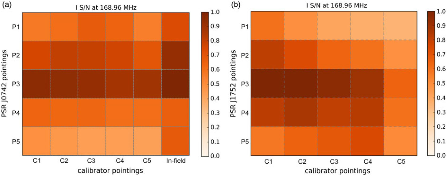
Figure 2. Signal-to-noise ratios of the total intensity pulse profiles at 168.96 MHz with a bandwidth of 1.28 MHz, for each of the five pulsar pointings calibrated using each of the five dedicated calibrator observations. All values are normalised to the maximum signal-to-noise ratio among the 25 combinations. (a) PSR J0742–2822 observations, (b) PSR J1752–2806 observations. Note that in-field calibration was not performed for PSR J1752–2806 (see Section 3.1 for details).
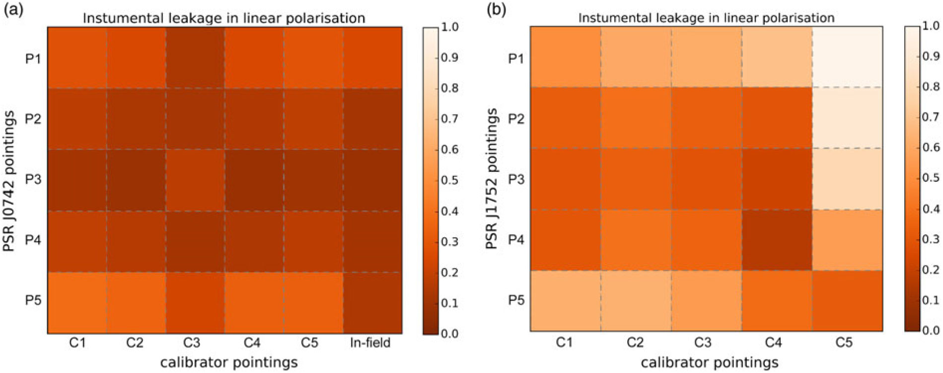
Figure 3. Fraction of instrumental polarisation leakage calculated using the RM CLEAN-ed Faraday spectra, for each of the five pulsar pointings calibrated using each of the five dedicated calibrator observations. (a) PSR J0742–2822 observations, (b) PSR J1752–2806 observations.
In summary, the in-field calibration performs well when both the sky model and the MWA beam model are sufficiently well determined. Towards lines-of-sight where this is not necessarily true, the dedicated calibrator observation is sufficient. We note that these are preliminary results based on two case studies, and a more detailed analysis involving a larger sample of pulsars would be useful to develop a higher degree of confidence. However, such an exercise is beyond the scope of this paper.
3.2. Reproducibility of pulse profiles
Here, we describe our analysis of the MWA tied-array data at different directions (Az, ZA), which shows that the polarimetric response is satisfactorily reliable for science, such as that demonstrated in the subsequent sections. The total intensities of the pulse profiles are found to be relatively stable, with a ˜10% variation in signal-to-noise, especially for calibrator observations where the source was less than 45° from the zenith, for example, Figures 2 and 3. The zenith pointing provides the pulse profile with the highest signal-to-noise ratio. This is consistent with our expectation because the MWA has maximum gain and the beam model is more accurately determined for pointings towards the zenith (except at frequencies higher than 270 MHz, see Section 6.2). The degree of linear polarisation (over the five different pointing positions and for each observing frequency between 150 and -270 MHz) varies by 8 ± 5% for PSR J0742–2822 and 4 ± 2% for PSR J1752–2806. Some of this discrepancy can be attributed to intrinsic pulse-to-pulse variations that contribute to the average pulse profile. The number of pulses within the short 5-min observations is ˜1 800 for PSR J0742–2822 and ˜500 for PSR J1752–2806. More than approximately 1 000 pulses are typically required to construct average pulse profiles that are stable, depending on the pulse phase-jitter properties of the pulsar (e.g. Liu et al. Reference Liu, Keane, Lee, Kramer, Cordes and Purver2012). Nevertheless, the profiles are also qualitatively similar, with the difference between the profiles attributable to the signal-to-noise ratios.
4. Faraday RM
We calculated the RM towards PSR J0742−2822 for all five observations separately (using the RM-CLEAN routine) to investigate the change in the apparent RM at different observing epochs and pointing directions. We also calculated the ionospheric Faraday rotation contribution for each observation. The results are summarised in Table 3. Before subtracting the ionospheric RM, the observed RM for PSR J0742−2822 ranged from 149.065 to 149.512 rad m−2 with a formal error of ˜0.05 rad m−2. After subtracting the ionospheric RM, the average RMISM for PSR J0742−2822 was estimated to be 150.915 ± 0.097 rad m−2. Thus, at these low frequencies, it is essential to correct for the ionospheric Faraday rotation, but the measurement uncertainty is dominated by the method currently used. Similarly, we determined the RM towards PSR J1752−2806 for all five 5-min observations and also for the 40-min observation centred at 118.40 MHz. Before subtracting the ionospheric RM, the observed RM ranged from 95.001 to 95.068 rad m−2. The measurement uncertainties for the five short observations are around 0.015 rad m−2, while for the observation centred at 118.40 MHz, the measurement uncertainty is only 0.01 rad m−2. The results are also summarised in Table 3.
Table 3. RM results for PSRs J0742-2822 and J1752-2806.
† This value is the observed RM, with no correction for the ionospheric RM value.
Figure 4 shows the RM CLEAN-ed Faraday spectra for PSR J1752−2806 from all five short observations and the 118.40 MHz observation. The height of the peak at 0 rad m−2, relative to the higher peak at the RM associated with the pulsar signal, indicates the fraction of instrumental polarisation leakage. We also show an example of an RM CLEAN-ed Faraday spectrum for the third short observation of PSR J0742−2822 in Figure 5.
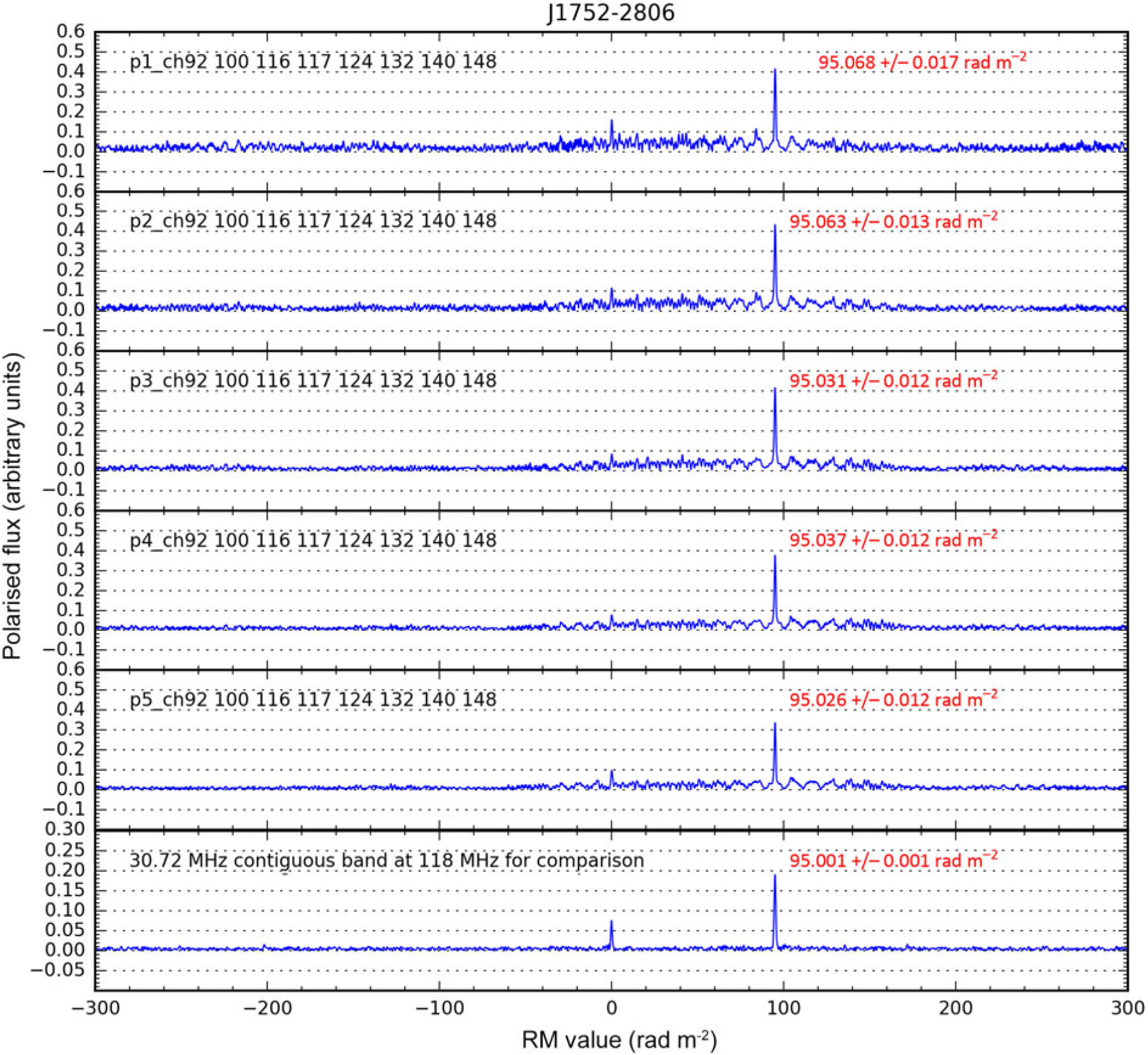
Figure 4. RM CLEAN-ed Faraday spectra for PSR J1752−2806. The labels in red show the observed RM prior to the subtraction of the ionospheric RM, and the uncertainty quoted is the formal error. The upper five panels show the Faraday spectra obtained from multiple short observations with observing frequencies 117.76–189.44 MHz. The bottom panel is the result from the observation centred at 118.40 MHz.
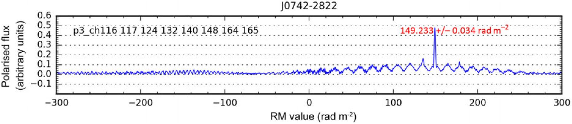
Figure 5. RM CLEAN-ed Faraday spectrum for PSR J0742−2822 using the third short observation (P3) with observing frequencies 148.48–211.20 MHz. The label in red is the observed RM prior to the subtraction of the ionospheric RM, and the uncertainty quoted is the formal error.
We note that the RM measurement uncertainty is proportional to the full width at half maximum (FWHM) of the rotation measure spread function (RMSF; analogous to a PSF in optical telescopes) and inversely proportional to the signal-to-noise ratio in the Faraday spectrum. The use of low frequencies and wide bandwidths reduces the FWHM of the RMSF, thus reducing the uncertainty on the RM measurement. At our lowest observing frequencies the pulsar profiles have lower signal-to-noise ratios, while at higher frequencies (particularly above 200 MHz), the instrumental polarisation leakage becomes greater (see Section 6.2). Including more of these higher-frequency channels increases the systematic error because the peaks associated with the pulsar signal and the instrumental polarisation in the Faraday spectrum calculated using each coarse frequency channel overlap due to the wider FWHM of the RMSF and increasing instrumental polarisation leakage. To achieve a balance between attaining smaller RM uncertainties by maximising the frequency range used, while reducing systematic errors from including high-frequency channels and noisier low-frequency channels, we adopted the frequency range 148.48–211.20 MHz to calculate the RM for PSR J0742−2822 and 117.76–189.44 MHz for PSR J1752−2806 (see Figures 6 and 8). For each pulsar, we calculated the Faraday spectrum for each coarse frequency channel individually to assist in deciding these optimum frequency ranges. We note that the RM measurements obtained for each channel (listed in Table 2) were all consistent within the formal errors.
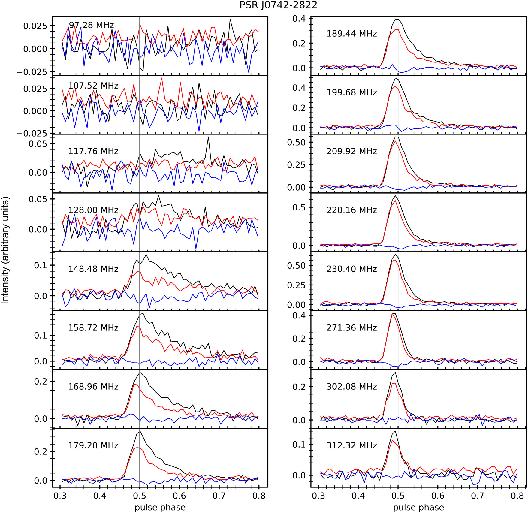
Figure 6. Polarimetric profiles for PSR J0742−2822 at frequencies from 97 to 313 MHz, each with a bandwidth of 1.28 MHz. Black lines indicate total intensity (Stokes I), red lines indicate linear polarisation (Stokes  $$\sqrt {{Q^2} + {U^2}} $$), and blue lines indicate circular polarisation (Stokes V). The data used here are the combination of all five short observations of PSR J0742−2822 and calibrated using the fifth calibration observation (C5). Note that the polarisation profiles above 270 MHz are increasingly affected by the instrumental polarisation leakage.
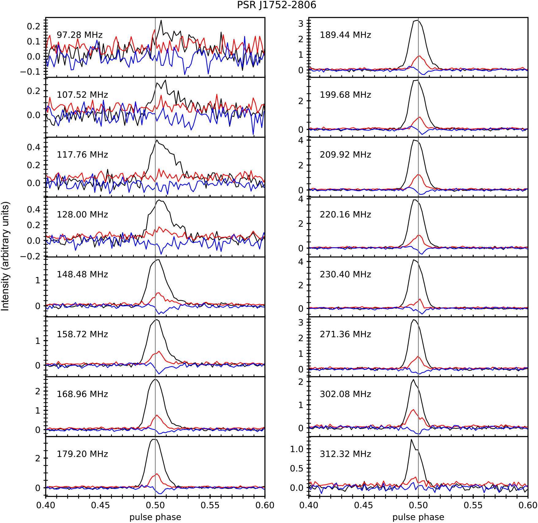
Figure 7. Polarimetric profile (lower panel) and PA curve (upper panel) for PSR J0742−2822. The black, red, and blue lines indicate the total intensity, linear polarisation, and circular polarisation, respectively. Here, we use the addition of nine 1.28 MHz channels between 148 and 211 MHz. The profile is generated using the data from all five observations, and calibrated using the fifth calibrator observation. The flux density is shown in arbitrary units.
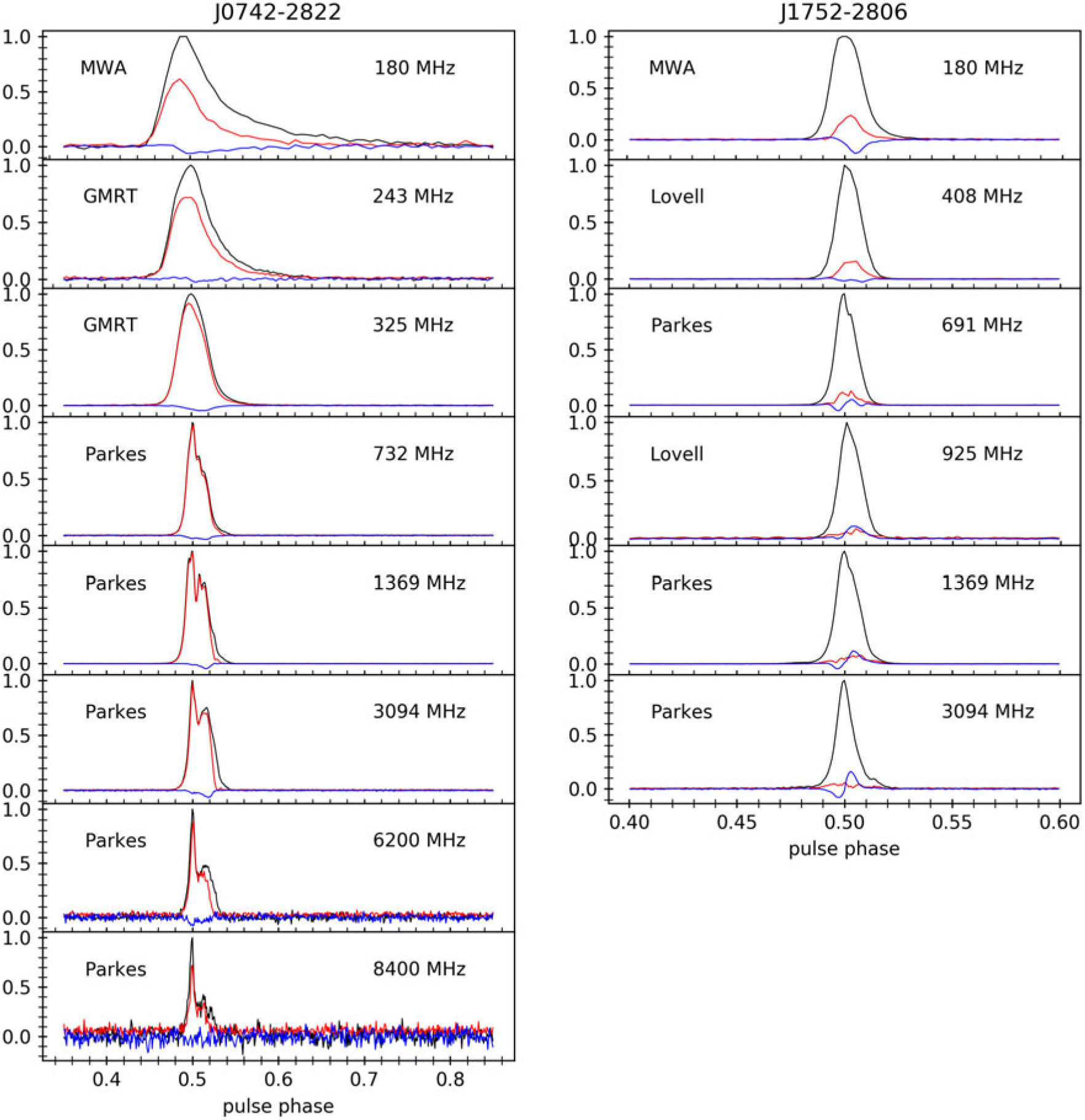
Figure 8. Polarimetric profiles for PSR J1752−2806 at frequencies from 97 to 313 MHz, each with a bandwidth of 1.28 MHz. Black lines indicate total intensity (Stokes I), red lines indicate linear polarisation (Stokes  $$\sqrt {{Q^2} + {U^2}} $$), and blue lines indicate circular polarisation (Stokes V). The data used here are the combination of all five short observations of PSR J1752−2806 and calibrated using the fourth calibration observation (C4). Note that the polarisation profiles above 270 MHz are increasingly affected by the instrumental polarisation leakage.
Using RM synthesis and the MWA’s large frequency lever arm, we are able to achieve higher precision on the RMs compared to previous studies at higher frequencies published in the literature. For example, the RM measured towards PSR J1752–2806 using the MWA data is more than twice as precise and in excellent agreement (0.5–σ) with the value reported in the pulsar catalogue from Hamilton & Lyne (Reference Hamilton and Lyne1987). As is evident from Table 3, the largest contribution to the RM uncertainty is the accuracy with which the ionospheric RM can be determined and corrected. Therefore, ongoing efforts to increase the accuracy of the ionospheric RM estimation are essential to fully realise the potential of high precision of RM measurements from low-frequency instruments (e.g. Malins et al. Reference Malins, White, Taylor, Stovall and Dowell2018).
5. Polarimetric profiles
5.1. PSR J0742−2822
We obtained polarimetric profiles for our target pulsars for a number of frequencies within the MWA’s operational frequency range. For PSR J0742−2822, the pulse profiles at the majority of the observing frequencies show significant exponential scattering tails, see Figure 6. The reduced telescope sensitivity and the increasing effects of scattering make it difficult to detect the pulsar at frequencies below 128 MHz. A detailed analysis of scattering properties of this pulsar can be found in Kirsten et al. (Reference Kirsten, Bhat, Meyers, Macquart, Tremblay and Ord2019). Despite the notable scattering, the pulse profile is highly linearly polarised at all frequencies, although the linear polarisation degree decreases towards lower frequencies. This may suggest that the scattering in the ISM gives rise to depolarisation of the pulsar emission; see Section 6.1 for further discussion.
Figure 7 shows the polarimetric profile of PSR J0742–2822 generated using the combined data from all five short observations over the frequency range 148–212 MHz (i.e. 9 × 1.28 MHz coarse channels). The PA curve shows a ˜50° swing and flattens towards later pulse phases in the scattering tail.
PSR J0742–2822 was also blindly detected in an all-sky survey of circular polarisation at 200 MHz with the MWA by Lenc et al. (Reference Lenc, Murphy, Lynch, Kaplan and Zhang2018). Their measured degree of circular polarisation, ≈−10%, is comparable with our estimation, −7 ± 18%. This result is also consistent with the ≈−7% circular polarisation from the Lovell telescope observation at 230 MHz (Gould & Lyne Reference Gould and Lyne1998).
5.2. PSR J1752−2806
Figure 8 shows the pulse profiles for PSR J1752−2806 from 97 to 312 MHz. The polarimetric profiles of PSR J1752–2806 show little evolution between 148 and 220 MHz, even though measurably longer scattering tails are seen towards the lower frequencies. The signal-to-noise ratio is comparatively lower at frequencies below 118 MHz. The profiles at 230 and 312 MHz show reduced linear polarisation while those at 271 and 302 MHz become dominated by instrumental leakage. This may be due to the increased instrumental leakage at frequencies above ≈270 MHz (cf. Sutinjo et al. Reference Sutinjo, O’Sullivan, Lenc, Wayth, Padhi, Hall and Tingay2015), see Section 6.2 for further discussion.
Figure 9 shows the polarimetric profiles for PSR J1752−2806 using the MWA data centred at 180 and 118 MHz. There appears to be a jump in the PA curve near the leading edge of the pulse profile, at both centre frequencies. This jump is ˜ 68 ± 8deg at 180 MHz and ˜ 59 ± 5 deg at 118 MHz. This jump also tentatively appears to coincide with a faint linear polarisation component at the leading edge of the pulse profile which is rather difficult to discern, given the time resolution of our data (see Table 2). Additional observations, high-quality low-frequency observations, will be useful to further investigate this.
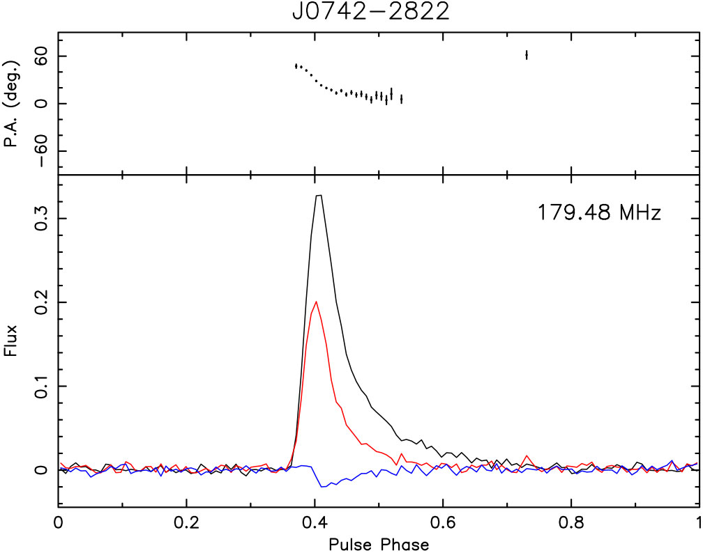
Figure 9. Polarimetric pulse profiles (lower panel) and PA curves (upper panel) for PSR J1752−2806. The black, red, and blue lines indicate the total intensity, linear polarisation, and circular polarisation, respectively. The flux densities are in arbitrary units. Left: the average profile for all five short observations for PSR J1752−2806, calibrated using the fourth calibrator observation (C4). Here, we use the addition of nine 1.28 MHz channels between 148 and 211 MHz. Right: the average profile from the MWA data centred at 118 MHz with 30.72 MHz contiguous bandwidth.
A closer examination of the polarimetric profiles at multiple MWA frequencies (Figure 8) reveals that the scattering effect is negligible for this pulsar above ˜150 MHz. However, as can be seen from Figure 9 (right panel), the pulse broadening arising from scattering is visibly strong at 118 MHz. Using the deconvolution method (as described in Bhat et al. Reference Bhat, Cordes and Chatterjee2003), we estimate the scatter broadening time to be 7.7 ± 0.7 ms at 118 MHz (assuming a one-side exponential for the pulse broadening function).
5.3. Comparison with the literature
Figure 10 shows the comparison between the polarimetric pulse profiles we obtained using the MWA and those available in the published literature. The MWA provides the lowest frequency pulse profiles. The profiles published in the literature provide additional data at frequencies up to 8 400 MHz for PSR J0742–2822 and up to 3 100 MHz for PSR J1752–2806.
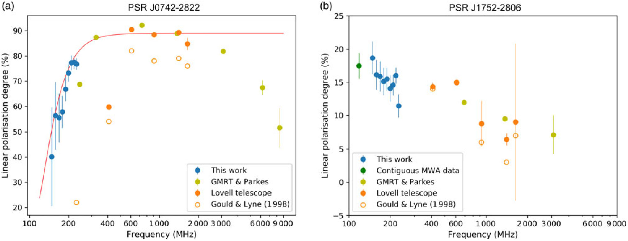
Figure 10. Polarimetric profiles for PSR J0742−2822 (left) and J1752−2806 (right) from the MWA and the literature (Gould & Lyne Reference Gould and Lyne1998; Karastergiou & Johnston Reference Karastergiou and Johnston2006; Johnston et al. Reference Johnston, Karastergiou and Willett2006, Reference Johnston, Kramer, Karastergiou, Hobbs, Ord and Wallman2007, Reference Johnston, Karastergiou, Mitra and Gupta2008). Black lines indicate the total intensity (Stokes I), red lines indicate linear polarisation (Stokes  $$\sqrt {{Q^2} + {U^2}} $$), and blue lines indicate circular polarisation (Stokes V). The flux density of each of the profiles is normalised (arbitrary units). The labels indicate the telescopes used to observe the pulsars and the centre observing frequencies.
For PSR J0742−2822, we obtained polarimetric profiles taken with the GMRT at 243 and 325 MHz (Johnston et al. Reference Johnston, Karastergiou, Mitra and Gupta2008) and Parkes profiles at 732, 1.4 , 3.1, 6.2, and 8.4 GHz (Karastergiou & Johnston Reference Karastergiou and Johnston2006; Johnston et al. Reference Johnston, Karastergiou and Willett2006). All of these are published in the literature, except for the 243, 325, 732, and 6200 MHz dataFootnote i. Pulse broadening (scattering) arising from multi-path propagation in the ISM can be clearly seen in the MWA and GMRT profiles. The emission is also highly linearly polarised, with a notable decrease towards lower frequencies; see Section 6.1 for further discussion.
For PSR J1752−2806, the literature archival data include those from the Lovell telescope (408 and 925 MHz; Gould & Lyne Reference Gould and Lyne1998) and Parkes (691, 1.4, 3.1; Karastergiou & Johnston Reference Karastergiou and Johnston2006; Johnston et al. Reference Johnston, Kramer, Karastergiou, Hobbs, Ord and Wallman2007). The linear polarisation fraction is smaller (<20%), compared to PSR J0742–2822, showing some profile evolution with increasing degrees of polarisation towards lower frequencies. In addition, the circular polarisation fraction is often comparable to that for the linear polarisation and also shows some evolution with frequency.
6. DISCUSSION
6.1. Frequency-dependent degree of linear polarisation
Figure 11 shows the measured degree of linear polarisation as a function of the observing frequency for PSR J0742–2822 (left) and PSR J1752−2806 (right). For PSR J1752−2806, the observed degree of linear polarisation increases towards lower frequencies, which is in line with the generally expected trend for pulsar emission. However, for PSR J0742–2822, the measured degree of linear polarisation peaks near 732 MHz, whereas it decreases gradually at frequencies ≳ 2 GHz, and quite rapidly at frequencies <300 MHz. This is in contradiction to the generally observed trend for many pulsars, where the degree of polarisation increases towards lower frequencies (e.g. Manchester Reference Manchester1971; Xilouris et al. Reference Xilouris, Kramer, Jessner, Wielebinski and Timofeev1996). We note, therefore, that the frequency-averaged polarisation profile in Figure 7 is purely for illustrative purpose, and that for any scientific interpretation, the profile evolution should be taken into account. For the frequency resolution that we have employed (10 kHz), bandwidth depolarisation is expected only for |RM| ≳ 400 rad m−2. Moreover, as can be seen in Figure 6, PSR J0742−2822 is also significantly scattered by the ISM. Therefore, it is possible that the depolarisation at low frequencies may due to scattering caused by the ISM.
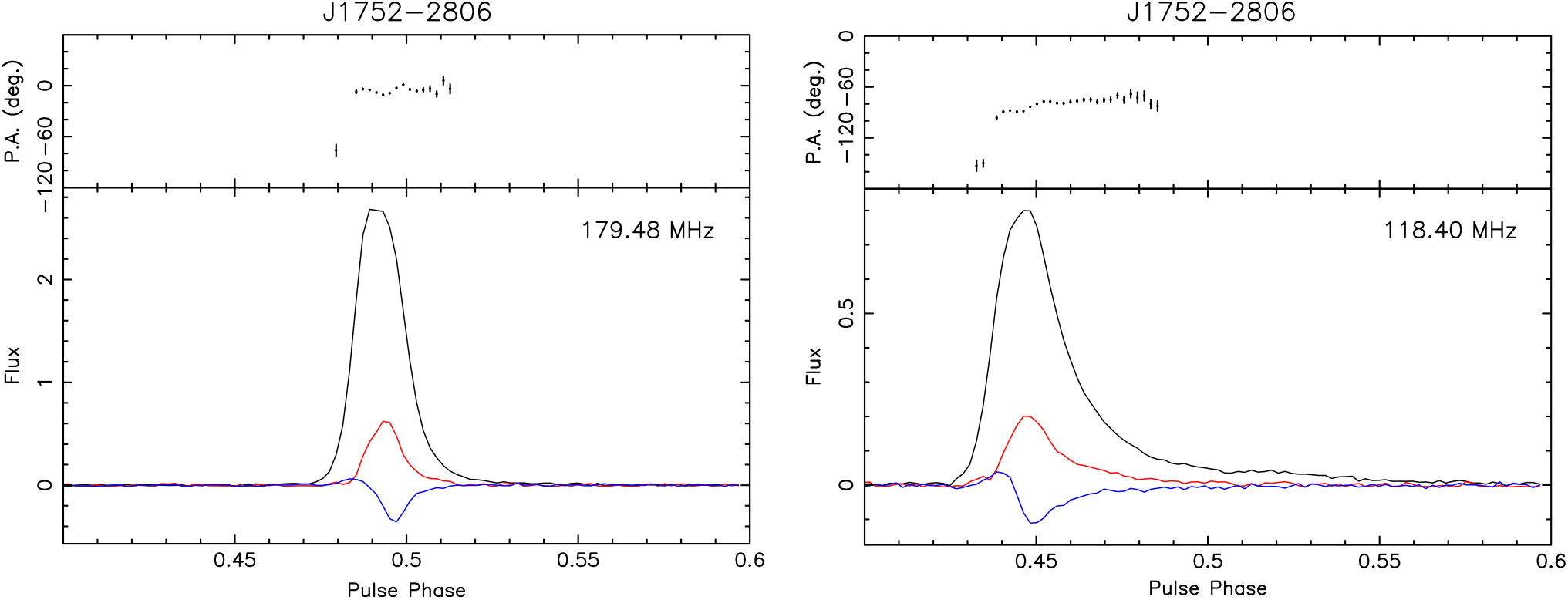
Figure 11. Degree of linear polarisation as function of frequency for PSR J0742–2822 (left) and PSR J1752−2806 (right). Blue points indicate the degree of linear polarisation using the MWA data between 148 and 230 MHz. Lime-green dots are from GMRT and Parkes data. Unfilled orange dots show the values published in Gould & Lyne (Reference Gould and Lyne1998) and filled orange dots are calculated using the profiles in Gould & Lyne (Reference Gould and Lyne1998). For PSR J1752–2806, the dark-green dot shows the linear polarisation observed with the MWA 118 MHz. For PSR J0742–2822 , the red line shows the depolarisation factor exp (− 2λ 4δRM2) fit where δRM=0.13radm2 (see Section 6.1).
There have been several studies in the literature discussing the impact of multi-path propagation in the ISM on the measured polarisation of pulsars (Komesaroff et al. Reference Komesaroff, Hamilton and Ables1972; Li&Han Reference Li and Han2003; Karastergiou Reference Karastergiou2009; Noutsos et al. Reference Noutsos, Karastergiou, Kramer, Johnston and Stappers2009, Reference Noutsos2015), which we will briefly review here. In early polarimetric studies of the Vela pulsar (PSR J0835−4510) from 300 to 1.4 GHz, Komesaroff et al. (Reference Komesaroff, Hamilton and Ables1972) measured a decrease in the degree of linear polarisation (at the pulse peak) and a smoother PA curve at their lower frequencies. While the smoother PA curve was interpreted as being due to scattering, the reduced degree in linear polarisation remained unexplained. Later, the work of Li & Han (Reference Li and Han2003) investigated the impact of scattering on the PA curves, and suggested that the scattering can potentially flatten the PA curves. Karastergiou (Reference Karastergiou2009) further investigated this effect by comparing the observed profiles for pulsars whose PA curves adhere to the RVM with simulated scattered profiles. Their work suggested that very modest amounts of scattering, together with orthogonal jumps, can lead to significant distortion in the PA curve. Noutsos et al. (Reference Noutsos, Karastergiou, Kramer, Johnston and Stappers2009) investigated phase-resolved RM variations for a sample of pulsars using 1.4 GHz Parkes data and suggested such variations can arise from interstellar scattering. This was further reinforced by Noutsos et al. (Reference Noutsos2015) using LOFAR data, who also found that three of their pulsars (two of which exhibit significant scattering) show a decrease in the degree of linear polarisation at low frequencies (<200 MHz).
For our MWA observations, the effective time resolution is mainly determined by the scattering time scale τ s. For example, at a frequency of 180 MHz, τ s is ˜ 6 ± 3 ms (Kirsten et al. Reference Kirsten, Bhat, Meyers, Macquart, Tremblay and Ord2019), which corresponds to 5 pulse phase bins given our sampling time resolution (see Table 2). This can potentially cause substantial smearing in polarisation profiles, leading to depolarisation. In such a scenario, a significant flattening of the PA curve is expected at lower frequencies, which is only seen in the trailing edge (in the scattering tail) of the pulse profile of PSR J0742−2822 (Figure 7). At earlier pulse phases, the PA curve shows structure in both the MWA and GMRT low-frequency data (<350 MHz).
We considered the possibility that this depolarisation could be caused by short-term variability in the ionospheric RM. However, if that is the case, the depolarisation factor should relate to the total observation time that we used to generate the polarimetric profiles. To this end, we examined the depolarisation for both short (a few minutes) and long time scales (a few hours), given the constraints of our observations. Specifically, we compared the depolarisation between (a) the addition of all five 5-min short observations and each individual 5-min observation; (b) the first and second halves of each 5-min observation. We found the depolarisation trends are consistent within the uncertainties. This indicates that the observed depolarisation is unlikely to be caused by the ionosphere. This is further reinforced by the fact that we see no significant depolarisation for PSR J1752−2806, and the ionosphere seems to show consistent behaviour between each pulsar’s observing epochs.
Depolarisation can also arise due to propagation through turbulent plasma components that are irregularly magnetised (e.g. Burn Reference Burn1966; Sokoloff et al. Reference Sokoloff, Bykov, Shukurov, Berkhuijsen, Beck and Poezd1998). In this case, stochastic Faraday rotation will depolarise the pulsar emission by a factor of exp(− 2λ 4δRM2) (e.g. Macquart & Melrose Reference Macquart and Melrose2000), where λ is the observing wavelength and δRM is the fluctuation in the RM. By fitting the observed degree of linear polarisation as a function of frequency, we estimate the required RM fluctuation δRM = 0.13 ± 0.02 rad m−2 (Figure 11). As previously mentioned, for PSR J0742−2822, τ s ˜ 6 ± 3 ms at 180 MHz (Kirsten et al. Reference Kirsten, Bhat, Meyers, Macquart, Tremblay and Ord2019). Johnston et al. (Reference Johnston, Nicastro and Koribalski1998) suggest that the scattering screen lies at a distance of ˜450 pc, associated with the Gum Nebula. In this case, the estimated size of the scattering disk is ˜33 AU. Given that there is typically a greater amount of turbulent structures seen in the general direction of the Gum Nebula, it is possible that the observed RM fluctuation is caused by small-scale, random magneto-ionic components (associated with turbulence) within the scattering screen. Further investigations are required to examine this in more detail and will be explored in a future publication.
6.2. Limitations of data reduction and future work
For the work presented here, we have used the MWA’s analytical beam model to calibrate and beamform the data. The analytical beam model is indeed a reasonably good approximation to the MWA’s tile beam, if we consider total intensity alone. For polarisation, the analytical beam model is acceptable (in terms of performance and stability) for observations at ZA ≲45° and at frequencies ≲270 MHz. Further developments have been made to the MWA tile beam model, including the recent fully embedded element (FEE) primary beam model (Sokolowski et al. Reference Sokolowski2017). This is a significant improvement to the analytical model and provides a more accurate prediction of the polarimetric response at large ZA. Therefore, using the FEE model in the calibration and beamforming will likely impart less instrumental polarimetric leakage to the data. This is illustrated in Figure 12, which shows the difference between the analytical and FEE beam models for the Stokes Q parameter, for example. The increasing deviation above 270 MHz indicates that the analytical beam model should be used with caution in this range.
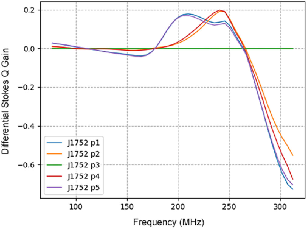
Figure 12. An example of the deviation in normalised Stokes Q gain value between the analytical and FEE beam models, as a function of observing frequency, for the directions of the five pointings towards PSR J1752–2806.
In future, we plan to extend this work through improved polarimetric calibration by integrating the FEE beam model into our calibration and beamforming pipeline. This is an important exercise, however, beyond the scope of the present work, given the much larger computational requirements of the FEE beam model. We also plan to compare the MWA beamformed data with the imaging products (e.g. Lenc et al. Reference Lenc2017), to provide further insights into the calibration and consistency between the observing modes, and to investigate any further corrections that could be applied to improve the polarimetric response.
7. SUMMARY
In this work, we have presented polarimetric studies of two bright southern pulsars, PSRs J0742–2822 and J1752–2806, using the MWA’s recently developed, full-polarisation, tied-array beam mode with high-time and high-frequency resolution. We have tested the response and stability of our calibration scheme over a range of ZA. Our analysis shows that the polarimetric response of the MWA is reliable in the domain where the analytical beam model is a good approximation to reality. This is satisfied when the observing frequency is less than 270 MHz and the ZA is less than 45°. As expected, observations closest to the zenith provide the highest signal-to-noise ratio pulse profiles.
For both PSRs J0742–2822 and J1752–2806, the profiles presented here are the first polarimetric profiles at frequencies below 300 MHz. We have studied the polarimetric pulse profile evolution over the frequency range 97–230 MHz using the MWA’s large (non-contiguous) fractional bandwidth and compared our results with the published work from higher frequency observations (up to ˜8.4 GHz). For PSR J0742–2822, the measured degree of linear polarisation shows a rapid decrease at low frequencies, which is in contrast with the generally expected trend for pulsar emission. This depolarisation trend may be attributed to stochastic Faraday rotation across the scattering disk.
In the near future, we plan to extend these studies for a larger sample of pulsars, building on the earlier work of Xue et al. (Reference Xue2017), in which we presented total intensity profiles of a large sample of pulsars using the MWA. The polarimetric profiles of a large sample of pulsars using the MWA will also serve as a useful reference for calibrating SKA-Low pulsar data.
Author ORCIDs
Mengyao Xue, https://orcid.org/0000-0001-8018-1830; S. M. Ord, https://orcid.org/0000-0002-6380-1425; S. E. Tremblay, https://orcid.org/0000-0001-7662-2576; N. D. R. Bhat, https://orcid.org/0000-0002-8383-5059; C. Sobey, https://orcid.org/0000-0002-8950-7873; B. W. Meyers, https://orcid.org/0000-0001-8845-1225; S. J. McSweeney, https://orcid.org/0000-0001-6114-7469; N. A. Swainston, https://orcid.org/0000-0001-8982-1187.
Acknowledgements
We thank Simon Johnston for kindly providing access to some of the unpublished data (for PSR J0742–2822), Jean-Pierre Macquart for the useful discussion on the depolarisation by the ISM, Willem van Straten for discussions relating to polarimetric analysis, and George Heald for providing the RM-CLEAN code. This scientific work makes use of the Murchison Radio-astronomy Observatory, operated by CSIRO. We acknowledge the Wajarri Yamatji people as the traditional owners of the Observatory site. Support for the operation of the MWA is provided by the Australian Government (NCRIS), under a contract to Curtin University administered by Astronomy Australia Limited. We acknowledge the Pawsey Supercomputing Centre which is supported by the Western Australian and Australian Governments. Parts of this research were supported by the Australian Research Council Centre of Excellence for All-sky Astrophysics (CAASTRO), through project number CE110001020. M. Xue is funded by the China Scholarship Council through the SKA PhD Scholarship project. BWM and SJM acknowledge the contribution of an Australian Government Research Training Program Scholarship in supporting this research.


