1. Introduction
With the first detection in gravitational and electromagnetic waves (Abbott et al. Reference Abbott2017a, Reference Abbott2017b), binary neutron star mergers promise to become outstanding sources of information for gravitational physics, astrophysics, and nuclear physics. Concerning the latter, already for decades, neutron stars (NS) represent a formidable source to improve our understanding of the properties of ultra-dense strongly interacting matter. This information will be complemented by the existing and upcoming observations of NS mergers. From the gravitational wave (GW) signal, the masses of the two objects can be determined. Additional information on matter properties can potentially be obtained from the tidal deformability during late inspiral (Faber & Rasio Reference Faber and Rasio2012; Read et al. Reference Raduta, Sedrakian and Weber2013), and, in particular, from the post-merger oscillations (Sekiguchi et al. Reference Sekiguchi, Kiuchi, Kyutoku and Shibata2011b; Bauswein et al. Reference Bauswein, Janka, Hebeler and Schwenk2012; Takami et al. Reference Takahashi2015; Bauswein et al. Reference Bauswein, Clark, Stergioulas and Janka2017). The observation of a correlated electromagnetic signal may also bring information on matter properties. There are indications that short gamma-ray bursts are only produced if a black hole (BH) is formed rapidly after merger (Fryer et al. Reference Fortin, Avancini, Providência and Vidaña2015; Lawrence et al. Reference Lattimer and Swesty2015), depending thus on the stability of the post-merger massive neutron star. A kilonova or a macronova event associated with the radioactive decay of produced r-process elements is determined by matter composition and ejecta masses (Hotokezaka et al. Reference Hempel, Fischer, Schaffner-Bielich and Liebendörfer2013). In a similar way, dissipative processes in the hot post-merger phase are controlled by matter composition and are crucial for the evolution of the merger remnant, see, for example, Alford et al. (Reference Alford, Bovard, Hanauske, Rezzolla and Schwenzer2018) and Fujibayashi et al. (Reference Fryer, Belczynski, Ramirez-Ruiz, Rosswog, Shen and Steiner2018).
Whereas neutron stars are essentially formed by catalysed cold β-equilibrated matter, temperatures as high as 50 MeV are expected during the evolution of the post-merger massive neutron star and its envelope (Sekiguchi et al. Reference Sekiguchi, Kiuchi, Kyutoku and Shibata2011b). The simulation of a merger event, where in addition β-equilibrium is not always achieved, requires, therefore, an equation of state (EoS) of warm stellar matter in a wide range of temperatures, electron fractions, and densities. Also, directly after its formation in a core-collapse supernova (CCSN), the newly born proto-neutron star evolves from matter with a quite large proton content to neutron-rich matter, emitting large amounts of neutrinos and reaching temperatures of up to 100 MeV (Burrows & Lattimer Reference Burrows and Lattimer1986; Keil & Janka Reference Ishizuka, Ohnishi, Tsubakihara, Sumiyoshi and Yamada1995; Pons et al. Reference Piekarewicz1999). Thus, for core-collapse simulations such an EoSFootnote a covering temperatures of 0 ≲ T ≲ 100 MeV, baryon number densities 10−11 fm−3 ≲ n B ≲ 10 fm−3 as well as electron fractions 0 ≲ Y e = n e/n B ≲ 0.6 is also essential.
The EoS by Lattimer & Swesty (Reference Lattimer and Swesty1991) (LS) and that by Shen et al. (Reference Shen, Toki, Oyamatsu and Sumiyoshi1998) (STOS) are the two most widely used general purpose models in simulations. Much effort has been devoted in the last years to improve these two classical models, see Oertel et al. (Reference Oertel, Hempel, Klähn and Typel2017) for a recent review. First, several EoS models have been proposed, which improve the treatment of non-homogeneous matter containing nuclear clusters at low densities and temperatures, for instance by Hempel & Schaffner-Bielich (Reference Hempel and Schaffner-Bielich2010), Raduta & Gulminelli (Reference Prakash, Bombaci, Prakash, Ellis, Lattimer and Knorren2010), Hempel et al. (Reference Hempel, Fischer, Schaffner-Bielich and Liebendörfer2012), Steiner, Hempel, & Fischer (Reference Steiner, Prakash, Lattimer and Ellis2013), and Gulminelli & Raduta (Reference Gal, Hungerford and Millener2015). Second, at high densities and temperatures non-nucleonic degrees of freedom such as hyperons, mesons, or quarks have been included into the EoS models, see, for example, Ishizuka et al. (Reference Ishizuka, Ohnishi, Tsubakihara, Sumiyoshi and Yamada2008), Nakazato, Sumiyoshi, & Yamada (Reference Miyatsu, Yamamuro and Nakazato2008), Sagert et al. (Reference Read, Baiotti, Creighton, Friedman and Giacomazzo2009), Shen et al. (Reference Shen, Toki, Oyamatsu and Sumiyoshi2011), Oertel, Fantina, & Novak (Reference Nakazato, Sumiyoshi and Yamada2012), and Banik, Hempel, & Bandyopadhyay (Reference Banik, Hempel and Bandyopadhyay2014).
However, additional degrees of freedom in the EoS lower the maximum neutron star mass, and it was only recently that the first EoS model (DD2Y) was proposed (Marques et al. Reference Lawrence, Tervala, Bedaque and Miller2017) containing the whole baryonic octet and being able to describe a cold neutron star with a mass of 2 M⊙ in agreement with observations ((Demorest et al. Reference Demorest, Pennucci, Ransom, Roberts and Hessels2010; Fonseca et al. Reference Fonseca2016; Antoniadis et al. Reference Antoniadis2013). The underlying nuclear model (DD2, Typel et al. Reference Tanigawa, Matsuzaki and Chiba2010) satisfies the presently accepted constraints on nuclear matter at saturation density and below obtained from nuclear experiments and theoretical calculations. Having in mind that it is important that simulations of supernovas or binary neutron star merging should include realistic EoS, and that accepted properties of nuclear matter are still defined within an interval of uncertainties, we propose in the present work two other EoS models containing the entire baryonic octet. These EoS have as underlying nuclear model SFHo (Steiner et al. Reference Steiner, Prakash, Lattimer and Ellis2013), a model which also satisfies the accepted constraints on nuclear matter. The main difference to DD2 is the smaller symmetry energy, leading among others, to a considerably lower prediction for the radius of a fiducial 1.4 M⊙ star: 11.9 km instead of 13.3 km obtained with DD2. Here, we will analyse how this property will influence the amount of hyperons inside hot and dense matter and the impact on thermodynamic properties.
Considering cold β-equilibrated NS, in general hyperons appear only in stars with a mass above roughly 1.4 M⊙, and then usually the overall fractions remain small if the 2 M⊙ maximum mass constraint is imposed, see for instance Fortin et al. (Reference Fonseca2016). It is, therefore, expected that they will not play a major role in determining global NS quantities such as the radii, moments of inertia, and tidal deformabilities. We emphasise, however, that the study of neutron stars, their formation process in CCSN, and their mergers is not restricted to the cold β-equilibrated EoS. Matter is heated up a lot in core-collapse and in the post-merger phase. Besides, the evolution of these processes requires the knowledge of transport properties such as the specific heat, viscosity, or neutrino emissivities that do depend on the constituents of matter. Hyperons may, as well, play an important role in NS cooling. It has been shown in Fortin et al. (Reference Fonseca2016) that several EoS that satisfy experimental and theoretical constraints up to saturation density do not allow for the fast cooling direct Urca process. In these cases, direct Urca processes only operate when hyperons appear, and, therefore, hyperons may have a strong influence on cooling; see also the recent study in Raduta, Sedrakian, & Weber (Reference Raduta and Gulminelli2018). Hyperons may also strongly affect the proto-neutron star cooling and stability and lead in particular to a delayed stellar mass BH formation, potentially observable via the associated neutrino signal (see, e.g. Keil & Janka Reference Ishizuka, Ohnishi, Tsubakihara, Sumiyoshi and Yamada1995; Prakash et al. Reference Pons, Steiner, Prakash and Lattimer1997; Pons et al. Reference Pons, Reddy, Prakash, Lattimer and Miralles2001; Peres, Oertel, & Novak Reference Oertel, Hempel, Klähn and Typel2013). In neutron star mergers too, hyperons may leave a clear imprint, see for instance Sekiguchi et al. (Reference Schaffner and Mishustin2011a). Note, however, that the employed EoS does not fulfil the 2 M⊙ constraint and hence that more work is necessary. Considering future neutron star merger detections, it is important to test all factors that might influence the final result, and hyperons are one of these factors.
The paper is organised as follows: in Section 2, the model for describing dense matter is presented; in Section 3, the properties of the two new hyperonic EoS based on SFHo are discussed and compared with the DD2Y model. In the last section, we summarise our results. Technical details on how the matching between clusterised and uniform matter is done, as well as technical issues concerning the EoS Tables in the COMPOSE data base, are given in the appendices.
2. Model for the EoS
Most available general purpose EoS models including the entire baryon octet and covering at the same time a sufficiently large range in baryon number density, n B, temperature T, and hadronic charge fraction, YQ = nQ/n B = Y eFootnote b in order to be applicable in CCSN or binary mergers are either not compatible with constraints from nuclear physics and/or a neutron star maximum mass of 2 M⊙; see the discussion in Oertel et al. (Reference Oertel, Hempel, Klähn and Typel2017). We will compare here two different EoSs, considering both all hyperons and being well compatible with the main present constraints: the DD2Y EoS (Marques et al. Reference Lawrence, Tervala, Bedaque and Miller2017) and a new EoS based on the nuclear SFHo EoS (Steiner et al. Reference Steiner, Prakash, Lattimer and Ellis2013), see below for details.
2.1. Description of inhomogeneous matter
The main aim of the present paper is to discuss the appearance of hyperons in high-density/high-temperature homogeneous matter and its impact on the EoS. In order to obtain a unified EoS over the entire needed range in temperature, baryon number density, and charge fraction, the present EoS models are combined with a description of inhomogeneous clustered matter at densities below roughly saturation density and low temperatures based on the respective nuclear interaction, using the statistical model by Hempel & Schaffner-Bielich (Hempel & Schaffner-Bielich Reference Heckel, Schneider and Sedrakian2010; Hempel et al. Reference Hempel and Schaffner-Bielich2012; Steiner et al. Reference Steiner, Prakash, Lattimer and Ellis2013). For a more detailed discussion of the issues related to clustered nuclear matter in stellar environments, see, for example, Raduta & Gulminelli (Reference Prakash, Bombaci, Prakash, Ellis, Lattimer and Knorren2010), Gulminelli & Raduta (Reference Gal, Hungerford and Millener2015), Hempel & Schaffner-Bielich (Reference Heckel, Schneider and Sedrakian2010), Typel et al. (Reference Typel, Röpke, Klähn, Blaschke and Wolter2010), Sumiyoshi & Röpke (Reference Sugahara and Toki2008), Buyukcizmeci, Botvina, & Mishustin (Reference Buyukcizmeci, Botvina and Mishustin2014), and Heckel, Schneider, & Sedrakian (Reference Hebeler, Lattimer, Pethick and Schwenk2009).
2.2. Homogeneous matter
We will treat homogeneous matter within two different phenomenological relativistic mean field (RMF) models. Baryonic interactions are modelled by the exchange of ‘meson’ fields. The term ‘meson’ refers thereby to the quantum numbers of the different interaction channels. The literature on those models is large and many different parameterisations exist (see, e.g. Dutra et al. Reference Dutra, Lourenço, Avancini, Carlson and Delfino2014).
We will use one model with density-dependent couplings and one model with nonlinear couplings of the meson fields. The Lagrangian density is written in the following form:
 \begin{eqnarray} {\mathcal L} &=& \sum_{j \in \mathcal{B}} \bar
\psi_j \left( i\gamma_\mu \partial^\mu - m_j + g_{\sigma j} \sigma
%+ g_{\sigma^* j} \sigma^*
\right. \\[3pt] & &- \left.
\,g_{\omega j} \gamma_\mu \omega^\mu - \,g_{\phi j} \gamma_\mu
\phi^\mu - \, g_{\rho j} \gamma_\mu \vec{\rho}^\mu \cdot
\vec{I}_j\right) \psi_j \nonumber \\[3pt] & &+\, \frac{1}{2}
(\partial_\mu \sigma \partial^\mu \sigma - m_\sigma^2 \sigma^2)
- \frac{g_2}{3} \sigma^3 - \frac{g_3}{4} \sigma^4 \nonumber \\[3pt] & &
-\, \frac{1}{4} W^\dagger_{\mu\nu} W^{\mu\nu} - \frac{1}{4}
P^\dagger_{\mu\nu} P^{\mu\nu} - \frac{1}{4} \vec{R}^\dagger_{\mu\nu}
\cdot \vec{R}^{\mu\nu} \nonumber \\[3pt] && +\, \frac{1}{2} m^2_\omega
\omega_\mu \omega^\mu + \frac{1}{2} m^2_\phi
\phi_\mu \phi^\mu + \frac{1}{2} m^2_\rho \vec{\rho}_\mu \cdot
\vec{\rho}^\mu\nonumber \\[3pt]
&& +\, \frac{c_3}{4} (\omega_\mu\omega^\mu)^2 + \frac{c_4}{4}
(\vec{\rho}_\mu \vec{\rho}^\mu)^2 + A(\sigma,\omega^\mu
\omega_\mu) \vec{\rho}^{\mu}\cdot\vec{\rho}_\mu,\nonumber
\end{eqnarray}
\begin{eqnarray} {\mathcal L} &=& \sum_{j \in \mathcal{B}} \bar
\psi_j \left( i\gamma_\mu \partial^\mu - m_j + g_{\sigma j} \sigma
%+ g_{\sigma^* j} \sigma^*
\right. \\[3pt] & &- \left.
\,g_{\omega j} \gamma_\mu \omega^\mu - \,g_{\phi j} \gamma_\mu
\phi^\mu - \, g_{\rho j} \gamma_\mu \vec{\rho}^\mu \cdot
\vec{I}_j\right) \psi_j \nonumber \\[3pt] & &+\, \frac{1}{2}
(\partial_\mu \sigma \partial^\mu \sigma - m_\sigma^2 \sigma^2)
- \frac{g_2}{3} \sigma^3 - \frac{g_3}{4} \sigma^4 \nonumber \\[3pt] & &
-\, \frac{1}{4} W^\dagger_{\mu\nu} W^{\mu\nu} - \frac{1}{4}
P^\dagger_{\mu\nu} P^{\mu\nu} - \frac{1}{4} \vec{R}^\dagger_{\mu\nu}
\cdot \vec{R}^{\mu\nu} \nonumber \\[3pt] && +\, \frac{1}{2} m^2_\omega
\omega_\mu \omega^\mu + \frac{1}{2} m^2_\phi
\phi_\mu \phi^\mu + \frac{1}{2} m^2_\rho \vec{\rho}_\mu \cdot
\vec{\rho}^\mu\nonumber \\[3pt]
&& +\, \frac{c_3}{4} (\omega_\mu\omega^\mu)^2 + \frac{c_4}{4}
(\vec{\rho}_\mu \vec{\rho}^\mu)^2 + A(\sigma,\omega^\mu
\omega_\mu) \vec{\rho}^{\mu}\cdot\vec{\rho}_\mu,\nonumber
\end{eqnarray}
where Ψj denotes the field of baryon j, and  $W_{\mu\nu},P_{\mu\nu}, \vec{R}_{\mu\nu}$ are the field tensors of the vector mesons, ɷ (isoscalar), ɸ (isoscalar), and ρ (isovector), of the form
 \begin{eqnarray}
V^{\mu\nu} = \partial^\mu V^\nu - \partial^\nu V^\mu.
\end{eqnarray}
\begin{eqnarray}
V^{\mu\nu} = \partial^\mu V^\nu - \partial^\nu V^\mu.
\end{eqnarray}
σ is a scalar–isoscalar meson field. For the baryon masses mj we have taken the following values: mn = 939.565346, mp = 938.272013, and m Λ = 1115.683, m Σ = 1190,  $m_{\Xi^-} = 1321.68, \ m_{\Xi^0} = 1314.83$ MeV ( $m_\Lambda = 1116.0, \ m_{\Sigma^{+,0,-}} = 1189.0,\ 1193.0, \ 1197.0, \ m_{\Xi^-} = 1321.0, \ m_{\Xi^0} = 1315.0$ MeV) for DD2Y (SFHoY).
The couplings of meson M to baryon j are conveniently written in the following form within models with density dependence:
 \begin{equation}
g_{Mj}(n_{\rm B}) = g_{Mj}(n_0) h_M(x)~,\quad x = n_{\rm B}/n_0~.
\end{equation}
\begin{equation}
g_{Mj}(n_{\rm B}) = g_{Mj}(n_0) h_M(x)~,\quad x = n_{\rm B}/n_0~.
\end{equation}
The density n 0 is thereby a normalisation constant, usually taken to be the saturation density n 0 = n sat of symmetric nuclear matter. Here, we will consider the DD2 parameterisation (Typel et al. Reference Tanigawa, Matsuzaki and Chiba2010), where the functions hM assume the following form for the isoscalar couplings (Typel et al. Reference Tanigawa, Matsuzaki and Chiba2010):
 \begin{equation}
h_M(x) = a_M \frac{1 + b_M ( x + d_M)^2}{1 + c_M (x + d_M)^2}
\end{equation}
\begin{equation}
h_M(x) = a_M \frac{1 + b_M ( x + d_M)^2}{1 + c_M (x + d_M)^2}
\end{equation}
and
 \begin{equation}
h_M(x) = \exp\kern-1pt[-a_M (x-1)] ~
\end{equation}
\begin{equation}
h_M(x) = \exp\kern-1pt[-a_M (x-1)] ~
\end{equation}
for the isovector ones. See Typel et al. (Reference Tanigawa, Matsuzaki and Chiba2010) for the values of the parameters aM, bM, cM and dM. The coupling constants of the nonlinear terms, g 2, g 3, c 3, c 4 and the function A are absent in models with density-dependent couplings.
The function
 \begin{equation}
A(\sigma,\omega_\mu \omega^\mu) = \sum_{i=1}^6 a_i \sigma^i + \sum_{j = 1}^3 b_j (\omega_\mu \omega^\mu)^j
\end{equation}
\begin{equation}
A(\sigma,\omega_\mu \omega^\mu) = \sum_{i=1}^6 a_i \sigma^i + \sum_{j = 1}^3 b_j (\omega_\mu \omega^\mu)^j
\end{equation}
in addition to the non-zero couplings g 2, g 3, c 3, and c 4 has been introduced in Steiner et al. (Reference Shlomo, Kolomietz and Colò2005) ( $A=g_\rho^2 f$ with f defined in Equation (15) of this reference) to be able to vary easily the symmetry energy in nonlinear models. Here, we employ the SFHo parameterisation (Steiner et al. Reference Steiner, Prakash, Lattimer and Ellis2013).
Both models will be used in mean field approximation, where the meson fields are replaced by their respective expectation values in uniform matter:
 \begin{eqnarray}
m_\sigma^2 \bar\sigma &=& \sum_{j \in B} g_{\sigma j} n_j^s - g_2 \bar\sigma^2 - g_3 \bar\sigma^3 + \frac{\partial A}{\partial \bar\sigma} \bar\rho^2\end{eqnarray}
\begin{eqnarray}
m_\sigma^2 \bar\sigma &=& \sum_{j \in B} g_{\sigma j} n_j^s - g_2 \bar\sigma^2 - g_3 \bar\sigma^3 + \frac{\partial A}{\partial \bar\sigma} \bar\rho^2\end{eqnarray}
 \begin{eqnarray}
m_\omega^2 \bar\omega &=& \sum_{j \in B} g_{\omega j} n_j - c_3 \bar\omega^3 - \frac{\partial A}{\partial \bar\omega} \bar\rho^2
\end{eqnarray}
\begin{eqnarray}
m_\omega^2 \bar\omega &=& \sum_{j \in B} g_{\omega j} n_j - c_3 \bar\omega^3 - \frac{\partial A}{\partial \bar\omega} \bar\rho^2
\end{eqnarray}
 \begin{eqnarray}
m_\phi^2 \bar\phi &=& \sum_{j \in B} g_{\phi j} n_j
\end{eqnarray}
\begin{eqnarray}
m_\phi^2 \bar\phi &=& \sum_{j \in B} g_{\phi j} n_j
\end{eqnarray}
 \begin{eqnarray}
m_\rho^2 \bar\rho &=& \sum_{j \in B} g_{\rho i} t_{3 j} n_j - c_4 \bar\rho^3 - 2 \, A\, \bar\rho,
\end{eqnarray}
\begin{eqnarray}
m_\rho^2 \bar\rho &=& \sum_{j \in B} g_{\rho i} t_{3 j} n_j - c_4 \bar\rho^3 - 2 \, A\, \bar\rho,
\end{eqnarray}
where  $\bar\rho=\langle\rho_3^0\rangle, \ \bar\omega=\langle\omega^0\rangle, \ \bar \phi=\langle\phi^0\rangle$, and t 3j represent the third component of isospin of baryon j with the convention that t 3p = 1/2. The scalar density of baryon j is given by
 \begin{equation}
n^s_j = \langle \bar \psi_j \psi_j \rangle = \frac{1}{\pi^2} \int
k^2 \frac{M^*_j} {\epsilon_j(k)} \{\kern1.5pt f[\epsilon_j(k)]
+\bar{f}[ \epsilon_j(k)] \} {\rm d}k,
\end{equation}
\begin{equation}
n^s_j = \langle \bar \psi_j \psi_j \rangle = \frac{1}{\pi^2} \int
k^2 \frac{M^*_j} {\epsilon_j(k)} \{\kern1.5pt f[\epsilon_j(k)]
+\bar{f}[ \epsilon_j(k)] \} {\rm d}k,
\end{equation}
and the number density by
 \begin{equation}
n_j = \langle \bar \psi_j\gamma^0 \psi_j \rangle = \frac{1}{\pi^2} \int
k^2 \{\kern1.5pt f[\epsilon_j(k)] - \bar{f}[\epsilon_j(k)]\}{\rm d}k.
\end{equation}
\begin{equation}
n_j = \langle \bar \psi_j\gamma^0 \psi_j \rangle = \frac{1}{\pi^2} \int
k^2 \{\kern1.5pt f[\epsilon_j(k)] - \bar{f}[\epsilon_j(k)]\}{\rm d}k.
\end{equation}
f and  $\bar{f}$ represent here the occupation numbers of the respective particle and antiparticle states with $\epsilon_j(k) = \sqrt{k^2 + M^{*2}_j}$, and effective chemical potentials $\mu^*_j$. They reduce to a step function at zero temperature. The effective baryon mass $M^*_j$ depends on the scalar mean fields as
 \begin{equation}
M^*_j = M_j - g_{\sigma j} \bar\sigma,
\end{equation}
\begin{equation}
M^*_j = M_j - g_{\sigma j} \bar\sigma,
\end{equation}
and the effective chemical potentials are related to the chemical potentials via
 \begin{equation}
\mu_j^* = \mu_j - g_{\omega j} \bar\omega - g_{\rho j} \,t_{3 j}
\bar\rho - g_{\phi j} \bar \phi - \Sigma_0^R.
\end{equation}
\begin{equation}
\mu_j^* = \mu_j - g_{\omega j} \bar\omega - g_{\rho j} \,t_{3 j}
\bar\rho - g_{\phi j} \bar \phi - \Sigma_0^R.
\end{equation}
The rearrangement term  $\Sigma_0^R$ is present in models with density-dependent couplings to ensure thermodynamic consistency. It is given by
 \begin{eqnarray}
\hspace*{-10pt}\Sigma_0^R = \sum_{j \in B} \left( \frac{\partial g_{\omega j}}{\partial n_j}
\bar\omega n_j + t_{3 j} \frac{\partial g_{\rho j}}{\partial n_j}
\bar\rho n_j +\frac{\partial g_{\phi j}}{\partial n_j}
\bar\phi n_j -\frac{\partial g_{\sigma j}}{\partial n_j}
\bar\sigma n_j^s \right)\!.
\end{eqnarray}
\begin{eqnarray}
\hspace*{-10pt}\Sigma_0^R = \sum_{j \in B} \left( \frac{\partial g_{\omega j}}{\partial n_j}
\bar\omega n_j + t_{3 j} \frac{\partial g_{\rho j}}{\partial n_j}
\bar\rho n_j +\frac{\partial g_{\phi j}}{\partial n_j}
\bar\phi n_j -\frac{\partial g_{\sigma j}}{\partial n_j}
\bar\sigma n_j^s \right)\!.
\end{eqnarray}
In contrast to the nuclear interaction which can be well constrained up to saturation density by information on nuclear properties, the information from hypernuclei is scarce and does not allow to fix the parameters of the model. In many recent works (Weissenborn, Chatterjee, & Schaffner-Bielich Reference Wang and Shen2012, Banik et al. Reference Banik, Hempel and Bandyopadhyay2014; Miyatsu, Yamamuro, & Nakazato Reference Menezes and Providência2013), the isoscalar vector meson–baryon coupling constants are hence related following a symmetry-inspired procedure such that the couplings of hyperons to isoscalar vector mesons are expressed in terms of gωN and a few additional parameters, see, for example, Schaffner & Mishustin (Reference Sagert, Fischer, Hempel, Pagliara, Schaffner-Bielich, Mezzacappa, Thielemann and Liebendörfer1996). In general, an underlying SU(6) symmetry and ideal ω–φ-mixing is assumed, completely fixing the hyperonic couplings in terms of gωN. Extending the above procedure to the isovector sector would lead to contradictions with the observed nuclear symmetry energy. gρN is therefore left as a free parameter and the remaining hyperonic isovector couplings are fixed by isospin symmetry.
This procedure has been adopted for the DD2Y model (Marques et al. Reference Lawrence, Tervala, Bedaque and Miller2017), but for the SFHo model with hyperons additional repulsion is needed such that the EoS for cold neutron star matter remains compatible with a maximum mass of 2 M⊙ as required by observations; see Section 3. We therefore rescale the ω and φ-meson–hyperon couplings as follows: gM Λ = 1.5gM Λ(SU(6)), gM Σ = 1.5gM Σ(SU(6)), gM Ξ = 1.875gM Ξ(SU(6)). This EoS model will be called ‘SFHoY’. In addition we will discuss the model with SU(6) couplings, called ‘SFHoY*’.
Comparing properties of single-Λ-hyperons with data on single Λ hypernuclei then allows to determine the remaining scalar coupling (van Dalen, Colucci, & Sedrakian Reference van Dalen, Colucci and Sedrakian2014; Fortin et al. Reference Fortin, Providencia, Raduta, Gulminelli, Zdunik, Haensel and Bejger2017). Less data are available for Ξ and Σ. An alternative, although less precise, way is to to use the values of hyperonic single-particle mean field potentials to constrain the scalar coupling constants. The potential for particle j in k-particle matter is given by
 \begin{equation}
U_j^{(k)}(n_k) = M^*_j - M_j + \mu_j - \mu^*_j~.
\end{equation}
\begin{equation}
U_j^{(k)}(n_k) = M^*_j - M_j + \mu_j - \mu^*_j~.
\end{equation}
We use here standard values at nuclear matter saturation density, n sat (Weissenborn et al. Reference Wang and Shen2012; Fortin et al. Reference Fortin, Providencia, Raduta, Gulminelli, Zdunik, Haensel and Bejger2017),  $U_\Lambda^{(N)}(n_{\mathrm{sat}})= -30$ MeV, $U_{\Xi}^{(N)}(n_{\mathrm{sat}}) = -18$ MeV (DD2Y) and −14 MeV (SFHoY), and $U_\Sigma^{(N)} (n_{\mathrm{sat}}) = + 30$ MeV. In Section 3.2 we will show that, in view of the uncertainties on the data, the obtained couplings are compatible with hypernuclear data.
Table 1 summarises the values of the meson–hyperon couplings in both models obtained from the above-described procedure.
Table 1. Coupling constants of the mesons to different hyperons within the three models presented here, normalised to the respective meson–nucleon coupling, that is, RMj = gMj/gMN, except for the φ-meson where the gωN coupling has been used for normalisation
3. EoS properties
3.1. Summary of constraints
Any model for the EoS has to be confronted with various constraints:
The recent observation of two massive neutron stars, indicating the maximum mass of a cold, non-, or slowly rotating (therefore spherically symmetric) neutron star should be above 2 M⊙, gives a very robust constraint on the interactions at supra-saturation densities.
Laboratory experiments on finite nuclei can constrain the EoS up to roughly saturation density. The main sources of information are nuclear mass measurements, neutron skin data, nuclear resonances, dipole polarisability of nuclei, nuclear decays, and heavy ion collisions. Experimental data can—within a model used for the analysis—be correlated with nuclear matter properties, which are in general chosen as the coefficients of a Taylor expansion of the energy per baryon of isospin symmetric nuclear matter around saturation. Values with a reasonable precision can be obtained for the saturation density (nsat), binding energy (E B), incompressibility (K), symmetry energy (Esym), and its slope (L). The extracted values depend of course on the model used for the analysis. In some cases, it has recently been shown that this model dependence can be reduced if values at n B = 0.1 fm−3 are given instead of saturation density (Khan & Margueron Reference Keil and Janka2013).
Much effort has recently been devoted to theoretical ab-initio calculations of pure neutron matter in order to constrain the EoS, and roughly up to saturation density, good agreement between the different approaches has been achieved. Since compact stars contain neutron-rich matter, this information is very interesting and completes the constraints on symmetric matter.
A summary and discussion of the most important available constraints can be found, for example, in Oertel et al. (Reference Oertel, Hempel, Klähn and Typel2017).
The two parameterisations chosen in this paper as basis for the EoS models, DD2 and SFHo, both agree reasonably well with most of the established constraints; see Table 2 for the values of different nuclear matter properties. For comparison, we show the values for two other interactions, that of the Lattimer and Swesty EoS (LS) (Lattimer & Swesty Reference Lattimer and Swesty1991) and that for the TM1 parameterisation (Sugahara & Toki Reference Sugahara and Toki1994), too. These two interactions have been employed in other recently developed general purpose EoS, including non-nucleonic degrees of freedom, for example, Ishizuka et al. (Reference Ishizuka, Ohnishi, Tsubakihara, Sumiyoshi and Yamada2008), Shen et al. (Reference Shen, Toki, Oyamatsu and Sumiyoshi2011), and Oertel et al. (Reference Nakazato, Sumiyoshi and Yamada2012).
Table 2. Nuclear matter properties of the two nuclear interaction models used within the different EoS models

Note: For comparison, the corresponding values of the interactions of the two standard EoS models, LS (Lattimer & Swesty Reference Lattimer and Swesty1991) and TM1 (Sugahara & Toki Reference Sugahara and Toki1994), are also given.
Saturation density, binding energy, and incompressibility of the two interactions used here lie within standard ranges (Oertel et al. Reference Oertel, Fantina and Novak2017): nsat≃0.15−0.16 fm−3, E B≃16 MeV, and K = 248±8 MeV (Piekarewicz Reference Peres, Oertel and Novak2004), and K = (240±20) MeV (Shlomo, Kolomietz, & Colò Reference Shen, Toki, Oyamatsu and Sumiyoshi2006). Note that in Stone, Stone, & Moszkowski (Reference Steiner, Hempel and Fischer2014), higher values of the incompressibility in the range 250–315 MeV are favoured. The last word is thus not said, but given the uncertainties, DD2 and SFHo still lie in within a reasonable range. The compatibility of Esym and L with ranges derived in Lattimer & Lim (Reference Khan and Margueron2013) (light gray rectangle) and in Oertel et al. (Reference Oertel, Fantina and Novak2017) (dark gray rectangle), respectively, are shown in Figure 1. In contrast to LS and TM1, the values of the two interactions employed here, DD2 and SFHo, are situated well within the rectangles.
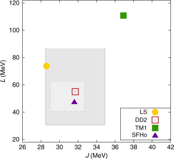
Figure 1. Values of Esym and L in different nuclear interaction models. The two gray rectangles correspond to the range for Esym and L derived in Lattimer & Lim (Reference Khan and Margueron2013) (light gray) and Oertel et al. (Reference Oertel, Fantina and Novak2017) (dark gray) from nuclear experiments and some neutron star observations.
In Figure 2, we display the density dependence of the symmetry energy obtained within the two parameterisations, DD2 and SFHo, which we have used as a basis to construct our EoS models. It is evident that DD2 produces a larger symmetry energy throughout the entire relevant density range. Neither the DD2 nor the SFHo allows for the nucleonic direct Urca process. This was already noted for DD2 in Fortin et al. (Reference Fonseca2016). Moreover, the authors of Fortin et al. (Reference Fonseca2016) identify the value L = 70 MeV as a limiting value below which the nucleonic direct Urca process would occur only in stars with a mass above 1.5 M⊙, and possibly simply not occur, depending on the model. The considered RMF models are in the latter case and satisfy the constraints obtained from microscopic calculations for neutron matter and the constraints on the saturation properties of nuclear matter. An exception in Fortin et al. (Reference Fonseca2016) is NL3ωρ which, however, only allows nucleonic direct Urca in stars with a mass above 2.5 M⊙. It is, therefore, not surprising that SFHo also shows a similar behaviour, since it satisfies the same constraints. With the opening of the hyperonic degrees of freedom, the hyperonic direct Urca becomes possible. For DD2 this is true for stars with M > 1.52 M⊙ with the onset of the Λ. For SFHoY (SFHoY*) the onset of the hyperon Ξ− (Λ) defines the onset of the hyperonic direct Urca and occurs for stars with M > 1.56 M⊙ (M > 1.26 M⊙). For SFHoY the Λ only sets in if M > 1.70 M⊙. It is expected that hyperon superfluidity will suppress neutrino emissivities due to hyperonic direct Urca processes. However, the superfluid hyperon gap is strongly dependent on the hyperon properties in neutron star matter and on the YY interaction (Wang & Shen Reference van Dalen, Colucci and Sedrakian2010). In particular, it has been shown the small value of ΔB ΛΛ obtained from  $^6_{\Lambda\Lambda}$ He (Takahashi et al. Reference Takahashi2001) leads to a very small gap in dense neutron matter (Tanigawa, Matsuzaki, & Chiba Reference Takami, Rezzolla and Baiotti2003) and in dense neutron star matter (Wang & Shen Reference van Dalen, Colucci and Sedrakian2010) or even suppresses completely the Λ superfluidity. Following Wang & Shen (Reference van Dalen, Colucci and Sedrakian2010), Λ superfluidity exists in massive neutron stars only for strong ΛΛ interactions. For the other hyperons, uncertainties are even larger; see also the discussion in Raduta et al. (Reference Raduta and Gulminelli2018). Therefore, at the present stage it is not possible to conclude which could be the role of hyperon superfluidity on the neutrino emissivity.
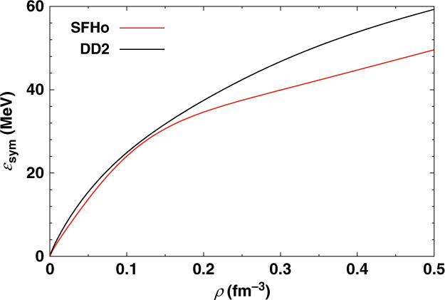
Figure 2. Symmetry energy as function of baryon number density within the two parameterisations employed here: SFHo and DD2.
As mentioned previously, ab-initio calculations of pure neutron matter can serve as a constraint on the EoS, too. Hence, in Figure 3 we show pressure and energy per baryon for pure neutron matter, comparing results from the different nuclear interactions with the ab-initio calculations from Hebeler et al. (Reference Gulminelli and Raduta2013), including an estimate of the corresponding uncertainties. None of the displayed models is in perfect agreement with the theoretical calculations; however, DD2 and SFHo show much better agreement than the standard LS and TM1 models. At densities below roughly n B = 0.1 fm−3, where the deviations of our models with the theoretical predictions are largest, one could in addition argue that the EoS of stellar matter is anyway strongly influenced by the treatment of nuclear clusters (nuclear masses, surface effects, thermal excitations, etc.) and the interaction model is not very important, see, for example, the discussion in Oertel et al. (Reference Oertel, Fantina and Novak2017).
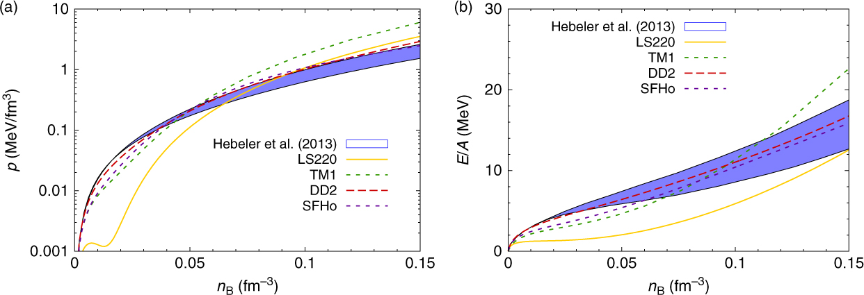
Figure 3. Pressure (a) and energy per baryon (b) of pure neutron matter as functions of baryon number density within different nuclear interaction models compared with the ab-initio calculations of Hebeler et al. (Reference Gulminelli and Raduta2013), indicated by the blue band.
In Figure 4, we display the mass–radius relation of coldFootnote c spherically symmetric neutron stars within different general purpose EoS models. In addition to the models containing the entire baryon octet discussed here, DD2Y (Marques et al. Reference Lawrence, Tervala, Bedaque and Miller2017), SFHoY, and SFHoY*, we show the purely nuclear LS EoS (Lattimer & Swesty Reference Lattimer and Lim1991), its extension with Λ-hyperons (LS220Λ) (Peres et al. Reference Oertel, Hempel, Klähn and Typel2013), the nuclear EoS by Shen et al. (STOS) employing the TM1 interaction (Shen et al. Reference Sekiguchi, Kiuchi, Kyutoku and Shibata1998), its extension with Λ-hyperons (STOSΛ) (Shen et al. Reference Shen, Yang and Toki2011) and all hyperons (STOSY) (Ishizuka et al. Reference Hotokezaka, Kyutoku, Tanaka, Kiuchi, Sekiguchi, Shibata and Wanajo2008), as well as one model including Λ-hyperons within DD2 from Banik et al. (Reference Banik, Hempel and Bandyopadhyay2014) (BHBΛφ). It is evident that among the EoS containing hyperons, apart from BHBΛφ which contains only Λ-hyperons, only the two EoS DD2Y and SFHoY are compatible with the 2 M⊙ constraint. A summary of cold neutron star properties for the different EoSs is given in Table 3.
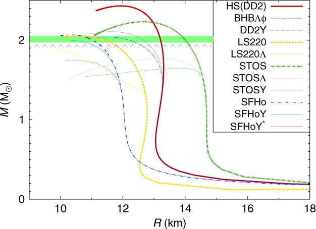
Figure 4. Gravitational mass versus circumferential equatorial radius for cold spherically symmetric neutron stars within different EoS models. The two horizontal bars indicate the two recent precise NS mass determinations, PSR J1614-2230 (Demorest et al. Reference Demorest, Pennucci, Ransom, Roberts and Hessels2010; Fonseca et al. Reference Fonseca2016) (hatched gray) and PSR J0348+0432 (Antoniadis et al. Reference Antoniadis2013) (green).
Table 3. Properties of cold spherically symmetric neutron stars in neutrinoless β-equilibrium: Maximum gravitational and baryonic masses, respectively, the total strangeness fraction, f S, representing the integral of the strangeness fraction Y S/3 over the whole star, defined as in Weissenborn et al. (Reference Wang and Shen2012), and the central baryon number density. The latter two quantities are given for the maximum mass configuration. In addition, the radius at a fiducial mass of Mg = 1.4 M⊙ is listed
Notes: For comparison with the hyperonic EoS DD2Y, SFHoY, and SFHoY*, the values for the purely nucleonic EoS models HS(DD2) (Fischer et al. Reference Faber and Rasio2014) and SFHo (Steiner et al. Reference Steiner, Prakash, Lattimer and Ellis2013), as well as the BHBΛφ EoS including Λ-hyperons based on HS(DD2) from Banik et al. (Reference Banik, Hempel and Bandyopadhyay2014), are also given.
3.2. Properties of Λ-hypernuclei
In this section, we study to which extent the hyperonic couplings of DD2Y and SFHoY reproduce experimental data of Λ-hypernuclei. To that end, we follow the approach of Fortin et al. (Reference Fortin, Providencia, Raduta, Gulminelli, Zdunik, Haensel and Bejger2017); see this reference for more details on the calculations. To calculate the binding energies of single and double Λ-hypernuclei, we have solved the Dirac equations for the nucleons and the Λ using the method described in Avancini et al. (Reference Avancini, Marinelli, Menezes, de Moraes and Providencia2007). A tensor term is included as in Shen, Yang, & Toki (Reference Shen, Toki, Oyamatsu and Sumiyoshi2006) in order to obtain a weak Λ-nuclear spin–orbit interaction. This term has no effect on homogeneous matter. As mentioned in the previous section, we assume the same density dependence for hyperon– and nucleon–meson couplings.
With the values of the coupling constants given in Table 1, the experimental binding energies B Λ of hypernuclei in s- and p-shells as given in Table IV of Gal, Hungerford, & Millener (Reference Fujibayashi, Kiuchi, Nishimura, Sekiguchi and Shibata2016) are well reproduced, for both models, DD2Y and SFHoY. The bond energy of  $_{\Lambda \Lambda}^6$He, the only known double-Λ hypernucleus, is, on the contrary, not well reproduced by both parameterisations. The reason is that the ΛΛ interaction is too repulsive at low densities.
In Marques et al. (Reference Lawrence, Tervala, Bedaque and Miller2017), a second parameterisation, DD2Yσ*, has been proposed, including the hidden strangeness meson σ*, coupling to hyperons and rendering the hyperon–hyperon (YY) interaction more attractive at low densities. Within DD2Yσ*, the bond energy comes out fine. But, the neutron star maximum mass, with a value of only 1.87 M⊙, does not fulfil the constraints from observations. At the present stage, we will keep the DD2Y parameterisation since developing a new hyperonic model based on the DD2 model is beyond the scope of the present paper. But, as indicated below, following the directions given in Fortin et al. (Reference Fortin, Providencia, Raduta, Gulminelli, Zdunik, Haensel and Bejger2017) for other models, parameterisations can be found in agreement with both the  $_{\Lambda \Lambda}^6$He bond energy and a neutron star mass of 2 M⊙ as well as the single-Λ hypernuclear data.
To that end, the SU(6) constraint on the isoscalar vector couplings has to be relaxed. This can be seen from Figure 5. For the top panels of that figure, the ratio R ωΛ has been fixed, and then the ratio R σΛ = gσ Λ/gσN has been fitted to the experimental binding energies B Λ of hypernuclei in the s- and p-shells and the coupling of the Λ to σ* to the bond energy of  $_{\Lambda\Lambda}^6$He; see Fortin et al. (Reference Fortin, Providencia, Raduta, Gulminelli, Zdunik, Haensel and Bejger2017) for details. The obtained neutron star maximum mass is then shown as a function of the value of Rφ Λ for several different cases. The lines labelled DD2-a (SFHo-a) thereby indicate the SU(6) value for Rω Λ and the arrows that for Rφ Λ, while the lines labelled DD2-b (SFHo-b) were obtained with Rω Λ = 1. The lower lines for each model correspond to models containing the entire baryon octet, whereas the upper lines correspond to models with Λ-hyperons only. In the sense that the onset of hyperons softens the EoS, and the softening is stronger the larger the number of hyperons included, the upper and lower curves of each model limit the maximum mass obtained with any hyperonic model almost independently of the details of the couplings of Ξ- and Σ-hyperons which are even less known than that for Λs due to the lack of relevant experimental data.
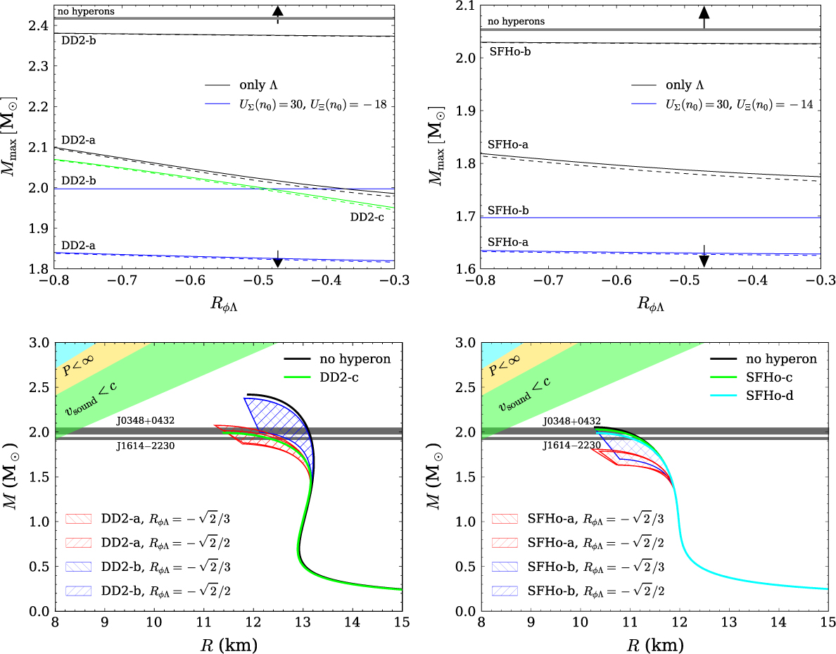
Figure 5. DD2-x (left) and SFHo-x (right) parameterisations. Top panels: neutron star maximum mass M max as a function of Rφ Λ for various hyperonic models. The values Rσ Λ, Rφ Λ, and Rσ* Λ are adjusted to reproduce the binding energies of single Λ-hypernuclei and of  $_{\Lambda\Lambda}^6$He with ΔBΛΛ = 0.50 MeV (solid lines) and 0.84 MeV (dashed lines). The arrows indicate the SU(6) value of Rφ Λ and the gray line the maximum mass for a purely nucleonic model. Bottom panels: MR curves for the parameterisations obtained for the models-a, that is, taking R Λω = 2/3 (red region) and the models-b, that is, with R Λω = 1 (blue region) for the two different values of R Λφ indicated in Table 4. In all cases, the upper limit is defined including only Λs and the bottom line including the complete baryonic octet with the couplings chosen as explained in the text. The black line is for pure nucleonic stars, and the green line is for the parameterisation of the set DD2-c (left) or SFHo-c (right); see the text for details. In the bottom-right panel, the cyan line identified as SFHo-d was obtained with the calibrated σ−Λ parameters for R Λω = 1 and the couplings to the Σ and Ξ as in the SFHoY model.
The lower curves of the top panel of Figure 5 were obtained taking the same couplings to the Λ-hyperon as model DD2-a (SFHo-a), and for the Ξ and Σ choosing the SU(6) coupling to the ω-meson and fitting the coupling to the σ-meson to obtain a single particle potential in nuclear matter of −18 MeV (−14 MeV) and +30 MeV, respectively. The coupling of these hyperons to the σ* and φ is taken equal to zero, and, therefore, we consider that the maximum mass determined with this prescription will define a lower limit, since, due to the dominance of the vector meson at high densities, it is expected that its repulsive effect will dominate over the attractive effect of σ*.
It is obvious that taking SU(6) values for the ω-couplings and not including the φ-meson for Ξ- and Σ-hyperons does not allow to reproduce the 2 M⊙ constraint. For DD2, we have, therefore, considered the effect of keeping the coupling of the Λ to all mesons as in DD2-a and, besides, coupling the Σ and Ξ also to the φ-meson keeping the SU(6) values for the vector mesons, these models are labelled DD2-c in the top-left panel of Figure 5. Under these conditions, it is possible to describe two solar mass stars for a large enough Rφ Λ. However, for SFHo, even taking only the Λ-hyperon with the Λ-meson coupling calibrated with the SU(6) values for the ω does not allow for a two solar mass star. Only breaking the SU(6) symmetry for both ω and φ vector-mesons the two solar masses constraint is satisfied.
In Table 4 we give, for two values of Rω Λ and two values of Rφ Λ, the calibrated values of Rσ Λ and Rσ* Λ. For reference, the corresponding values of the Λ-potential in symmetric baryonic matter at saturation  $U_\Lambda^{(N)}(n_{\mathrm{sat}})$ obtained from Equation (16) are given as well as $U_{\Lambda}^{(\Lambda)}(n_{\mathrm{sat}})$, and $U_{\Lambda}^{(\Lambda)}(n_{\mathrm{sat}}/5)$, the Λ single-particle potential in Λ-matter. It is interesting to notice that for DD2 $U_{\Lambda}^{(\Lambda)} (n_{\mathrm{sat}}/5) $ is close to the value of −5 MeV, as generally used in the literature to fix these couplings.
Table 4. Calibration to Λ-hypernuclei and  $_{\Lambda\Lambda}^6$He for models with the SU (6) value, Rω Λ = 2/3 (a), and Rω Λ = 1 (b)
Notes: For a given Rω Λ, values of Rσ Λ are calibrated to reproduce the binding energies B Λ of single hypernuclei in the s- and p-shells. The value of the Λ-potential in symmetric baryonic matter at saturation is given for reference. For given Rφ Λ, Rσ* Λ are calibrated to reproduce the upper and lower values of the bond energy of  $_{\Lambda \Lambda}^6$He. For reference, the Λ-potential in pure Λ-matter at saturation and at n sat/5 is also given. All energies are given in MeV.
In order to better understand the predictions obtained for the neutron stars mass–radius relation, we display in Figure 5 (bottom panels) the complete M−R curves and illustrate with a hashed region, the region limited by the upper and lower limits shown in the top panels of the same figure. The black line represents pure nucleonic stars. We also include in the figure the constraints imposed by the two pulsars PSR J1614-2230 (Demorest et al. Reference Demorest, Pennucci, Ransom, Roberts and Hessels2010; Fonseca et al. Reference Fonseca2016) and PSR J0348+0432 (Antoniadis et al. Reference Antoniadis2013). All configurations obtained with the larger ω couplings are within the observed masses, while for the SU(6)-couplings some configurations could be too small.
The green line in the bottom-left panel labelled DD2-c was calculated taking for the φ-couplings the SU(6) values. A maximum mass of 1.99 M⊙ is obtained, just slightly smaller than the maximum mass determined with DD2Y and clearly above DD2Yσ*, where Ξ- and Σ-hyperons couple to σ*, too. This last difference can be attributed to the fact that DD2Yσ* has a much larger fraction of negatively charged hyperons and, therefore, smaller amount of electrons.
For the SFHo model, two extra M−R curves are shown in the bottom-right panel with different choices for the vector–meson couplings, the models labelled SFHo-c (green) and SFHo-d (cyan). The SFHo-c model with calibrated Λ-couplings to hypernuclei and the Σ and Ξ potentials in symmetric matter as above has ratios Rωi = 1 for all hyperons and Rφ Λ = Rφ Σ = −0.707 and Rφ Ξ = −1.77, and predicts a maximum mass of 2.03 M⊙, slightly above the one given by SFHoY, very close to the maximum mass obtained including only calibrated Λs, see the top curves for SFHo-b in top-right panel of Figure 5. The SFHo-d model was obtained with the calibrated Λ parameters with R Λω = 1 and Rφ Λ = −0.707 and the couplings to the Σ and Ξ as in the SFHoY model. Star properties obtained with this model are very similar to the ones obtained with SFHoY.
3.3. Hyperon content and thermodynamic properties
Let us now discuss the properties of homogeneous matter obtained within the different EoS models, DD2Y, SFHoY, and SFHoY*. Although there are small quantitative differences, the regions in temperature and baryon number density, where the overall hyperon fraction exceeds 10−4, see Figure 6, have a very similar shape in the different models. The bump in the curves, that is, the part of the lines above approximately 20 MeV, where the abundance of hyperons is still below 10−4, arises from the competition between light nuclear clusters and hyperons in this particular temperature and density domain and does not exist in the EoSs built on nuclear models without light clusters; see Oertel et al. (Reference Oertel, Fantina and Novak2017). In a more complete model, where light clusters and hyperons are allowed to coexist, the bump would probably disappear, and above a temperature of roughly 20 MeV, hyperons would exist at any density. In Menezes & Providência (Reference Marques, Oertel, Hempel and Novak2017), hyperon fractions have been calculated in the presence of heavy clusters. Under these conditions these fractions were always below 10−5. However, heavy clusters melt at quite low temperatures, so it is important to also include light clusters explicitly. At large temperatures, results are almost insensitive to the interaction but do depend on the number of competing species, such that the hyperon onset temperature is very similar within all models.
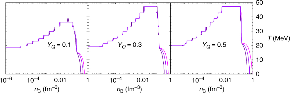
Figure 6. The lines delimit the regions in temperature and baryon number density for which the overall hyperon fraction exceeds 10−4, which are situated above the lines. Different charge fractions are shown as indicated within the panels. The lines correspond to DD2Y, SFHoY*, and SFHoY, respectively, appearing in that order at low temperatures and high densities.
The main differences between models occur at low temperatures when the results are sensitive to the hyperon–meson interactions. Thus, in particular for cold neutron stars, the hyperon onset density is lower in DD2Y than in SFHoY. There are two reasons for that. First, being consistent with the 2 M⊙ constraint suppresses hyperonic degrees of freedom at high density and low temperatures. Therefore in model SFHoY*, with SU(6) couplings and thus less repulsion than SFHoY, hyperons appear at lower densities. Second, the smaller symmetry energy in SFHo compared with DD2, see Figure 2, effectively disfavours hyperons with respect to nucleons.
Let us discuss these assertions now in more detail. In Figure 7, the hyperon fractions are plotted as a function of the baryonic density for different electron fractions and T = 30 MeV. DD2Y clearly has the largest overall hyperon fractions. Again, this can be due to the larger couplings to vector mesons in the SFHoY model and to the smaller symmetry energy of SHFo to DD2 for all densities. Comparing SFHoY and SFHoY* corroborates these arguments: the latter has larger hyperon fractions due to less repulsive couplings, but does not reach DD2Y due to the smaller symmetry energy. In all three models, due to the high temperature, the hyperon onset density is very similar and strongly correlated with the disappearance of nuclear clusters in favour of homogeneous matter. Within DD2Y, above the onset density, the overall hyperon fraction strongly increases with density. This is slightly less true for SFHoY* and much less for SFHoY, where the additional repulsion for hyperons more strongly affects the results at high densities.
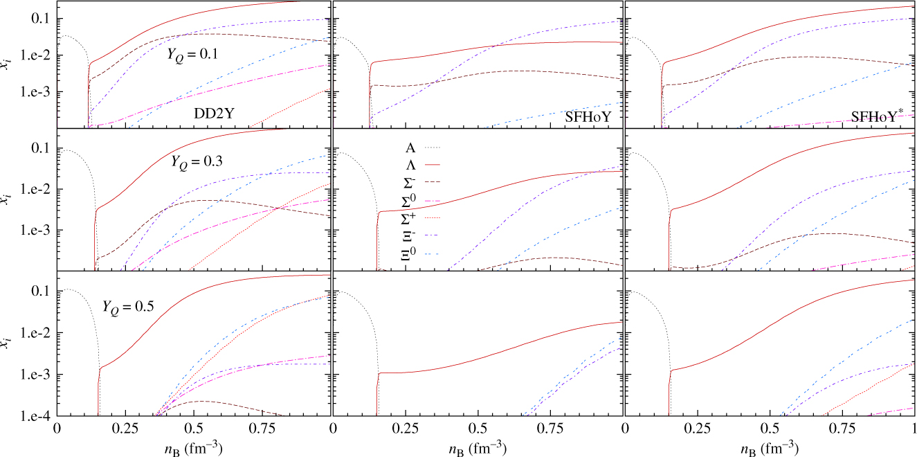
Figure 7. Particle fractions versus baryonic density for DD2Y (left), SFHoY (middle), and SFHoY* (right) for T = 30 MeV and different charge fractions. The label ‘A’ indicates the sum over all different nuclei.
The three most abundant hyperons obtained within all models at YQ = 0.1 coincide: Λ, Ξ−, and Σ−. Λ has the smallest mass and the abundance of the two other is due to the well-known negative isospin projection, favouring negatively charged particles in matter with low charge fractions. It is interesting to see that Ξ− in SFHoY is as abundant as in DD2Y at large densities, and contrary to DD2Y they become more abundant than Λ-hyperons. The reason is that with our proposal the couplings of the Ξ are less increased with respect to the SU(6) values than for the other hyperons, and as a consequence at large densities and for very asymmetric matter the Ξ-hyperons become preferred even to the much less massive Λ. In SFHoY*, where SU(6)-couplings are employed, still Λ-hyperons remain most abundant at high densities, although the smaller symmetry energy in SFHo with respect to DD2 more strongly favours negatively charged particles at low YQ.
With increasing charge fraction YQ, neutral and positively charged hyperons and less massive ones are favoured. For YQ = 0.5, apart from Λ-hyperons, the two most abundant hyperons are Ξ0 and Ξ+ followed by Ξ− for DD2Y. For SFHoY, Ξ0 and Ξ− are the most abundant and the Σs are not present: again repulsion is too strong for Σ-hyperons.
In Figure 8 we plot the hyperon fractions obtained within DD2Y as a function of the charge fraction for T = 50 MeV and n B = 0.1 and 0.3 fm−3. The hyperon Λ is the most abundant for all fractions shown except for very small fractions and n B = 0.1 fm−3: this is the hyperon with the lowest mass and the most bound in symmetric nuclear matter. However, the abundance of the isoscalar Λ only moderately depends on YQ, and for very small YQ,  $x_{\Sigma^-}$ exceeds x Λ. With decreasing charge fraction, the charge chemical potential decreases, favouring thus negatively charged particles, Σ− and Ξ−. In the present RMF models this is expressed via the coupling to the ρ-meson. Inversely, $x_{\Sigma^+}$ increases with increasing charge fraction. On the other extreme, for YQ ∼ 0.5, the abundance of the different hyperon species mainly depends on their mass, such that $x_{\Sigma^+}>x_{\Sigma^-}$. At this high temperatures, the hyperonic interactions only marginally influence the ordering of the hyperons. At T = 0, where interactions are important, the first hyperon to set in is the Λ followed by the Ξ−. The effect of temperature, which favours hyperons with smaller masses, is larger for the smaller densities, and this explains why the difference between Σ− and Ξ− is larger for n B = 0.1 fm−3 than for n B = 0.3 fm−3. Results obtained within the other two models are very similar, the ordering of the hyperons being the same, the only difference being the abundances that are smaller, in particular for SFHoY.
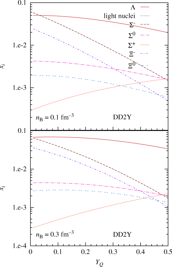
Figure 8. Hyperon fractions versus charge fraction YQ for DD2Y for T = 50 MeV and different baryonic densities.
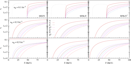
The effect of temperature is better understood from Figure 9, where we display the particle fractions as a function of temperature for a reference charge fraction, YQ = 0.3, and three values of the baryonic density. Some common features are present in all the three models. For the lowest temperatures, the same sequence of hyperons occurs with respect to their abundance in all models but the smallest abundance is obtained for SFHoY, followed by SFHoY* and DD2Y. At large temperatures, the Σ+ and the Ξ0 become more abundant than their neutral or negatively charged counterparts Σ0 and Ξ− if the density is not too large. This change of abundance will occur at lower temperatures for DD2Y, followed by SFHoY* and finally SFHoY. A quite different picture is described at T = 100 MeV and n B = 0.5 fm−3 by DD2Y where all fractions, except for Λ hyperons, coincide in contrast to the two other models. With SFHoY, the fraction of Σ+ is still the lowest and about 0.25 smaller than  $x_{\Xi^-}$. This is a consequence of the smaller symmetry energy in the two models based on SFHo and the larger repulsion felt by hyperons in SFHoY. In this model, the same scenario of equal fractions is pushed to higher temperatures and/or densities. It is clear that the abundances change as function of the different density values and, in particular, the most abundant hyperon after the Λ is the Σ− for the two lower densities and the Ξ− for n B = 0.5 fm−3. This change is related to the fact that at low densities and high temperatures, the interactions only slightly influence the abundances, which are mostly given by masses. At high densities, as seen here for n B = 0.5 fm−3(bottom panels), we approach the situation at zero temperature discussed before where interactions are important and Ξ− becomes the first hyperon to set after Λ’s.
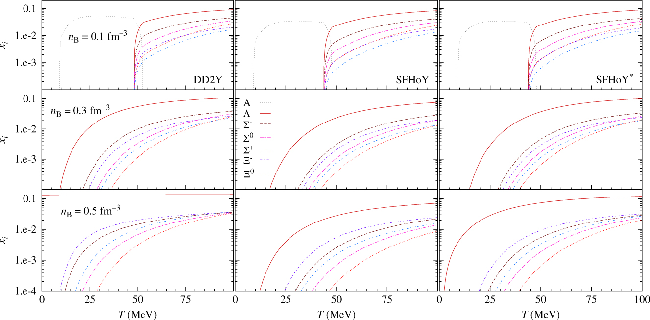
Figure 9. Particle fractions as a function of the temperature for different values of fixed baryon number density and charge fraction YQ = 0.3 within DD2Y (left), SFHoY (middle), and SFHoY* (right) EoS.
Obviously, large hyperon abundances have strong effects on thermodynamic quantities, too. Hence, as can be seen from Figure 10, pressure and free energy per baryon are considerably reduced above roughly 2–3 times nuclear saturation density in the models with hyperons compared with the purely nucleonic ones. The reduction is most important for low electron fractions. This is clearly understandable since, as seen before, the overall hyperon fractions are highest for small electron fractions. The higher hyperon fractions in DD2Y compared with SFHoY* and, in particular, SFHoY explain the larger reduction within DD2Y (and SFHoY*) too. As already discussed in Marques et al. (Reference Lawrence, Tervala, Bedaque and Miller2017), only a small further reduction in DD2Y with respect to BHBΛφ can be observed. This is due to the fact that the overall hyperon fraction is very similar in both models, the additional hyperonic degrees of freedom in DD2Y being compensated by a higher Λ-fraction in BHBΛφ. When comparing SFHoY and SFHoY* the reduction is larger in the second model because higher hyperon fractions are present due to the less repulsive hyperonic interactions.
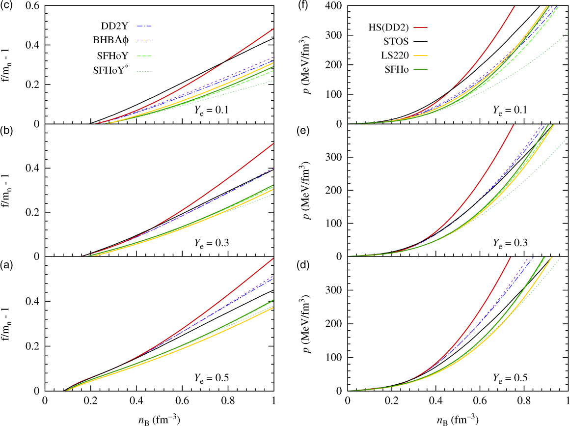
Figure 10. Pressure (panels d–f) and normalised free energy per baryon (panels a–c) as function of baryon number density for different values of fixed electron fraction and T = 30 MeV within different EoS. Contributions from electrons/positrons and photons are included, demanding overall charge neutrality, that is, Y e = YQ. For information, the pressure in the classical models LS220 and STOS is displayed in addition.
In Figure 11, pressure and free energy are plotted as function of temperature for different values of n B and an intermediate value of Y e = 0.3. The results again confirm our findings: the presence of hyperonic degrees of freedom reduces pressure and free energy with its impact increasing with temperature, as the hyperon fractions increase. Again, the effect is less pronounced in SFHoY, since for the density values shown, the more strongly repulsive hyperonic interactions diminish the influence of hyperons within this model. As can be seen comparing SFHoY* and DD2Y, the smaller symmetry energy within SFHo also plays a non-negligible role in rendering hyperons less important within the models based on SFHo.
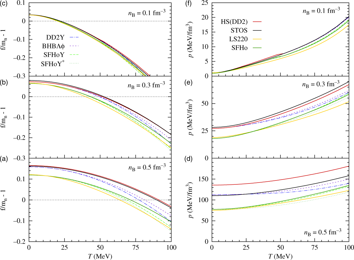
Figure 11. Same as Figure 10, but as function of temperature for Y e = 0.3 and different fixed values of n B.
The fraction of hyperons and the way they are distributed among the different species at a given temperature will affect the entropy per baryon, s B, of the system, too. If the energy is shared among an increased number of degrees of freedom, thermal excitations will be reduced for each of them and entropy will be higher for systems with hyperons than for purely nucleonic ones at a given temperature. On the other hand, for a given s B, we expect a lower temperature in systems with hyperons. This is confirmed by the results shown in Figures 12 and 13, where temperature as function of baryon number density for three different values of entropy per baryon (s B = 1,2,4) is displayed. These entropy values correspond to typical values in proto-neutron stars. In Figure 12, the overall lepton fraction (including neutrinos) has been fixed to Y L = 0.4, again a typical value for proto-neutron stars before neutrinos diffuse out of the star. In Figure 13, the same quantities are plotted for β-equilibrated stellar matter with no trapped neutrinos. In this figure we also include for reference the results for LS220 and STOS. As expected, as soon as hyperons set in, the temperature drops. This effect is more pronounced within DD2Y due to the larger amount of hyperons. Comparing Figures 12 and 13, it can be seen that for matter without neutrinos, temperatures are generally larger since due to the absence of neutrinos, there is one degree of freedom less. In this case hyperons set in at very low densities; the larger the entropy the lower the onset density.
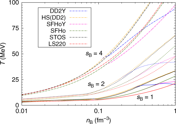
Figure 12. Temperature as function of the baryon number density for different values of fixed entropy per baryon: s B = 1 (plain lines), s B = 2 (dashed lines), and s B = 4 (dash-dotted lines) comparing purely nucleonic models with hyperonic ones, HD(DD2) and DD2Y, as well as SFHo and SFHoY. The lepton fraction has been fixed to Y L = 0.4.
It is interesting to notice that already if only nucleons are considered, the two models show non-negligible differences. SFHo predicts lower temperatures than DD2 both for matter with trapped and neutrino-free matter (see Figures 12 and 13). This is probably due to the differences in the symmetry energy: a smaller symmetry energy leads to lower proton fractions and, thus, electron fractions, leading to a lower temperature for a given entropy per baryon. The effect is slightly more pronounced at fixed lepton fraction, since a lower electron fraction corresponds to a larger neutrino fraction within the SFHo model, too, lowering additionally the temperature needed for a given entropy per baryon. Comparing STOS and LS220 results with the above ones we observe that: (a) the temperatures predicted by STOS are similar to DD2, being only slightly smaller at large densities; (b) LS220 predicts smaller temperatures than the other nuclear models. The temperatures remain even below those predicted by the hyperonic models in a large density range.
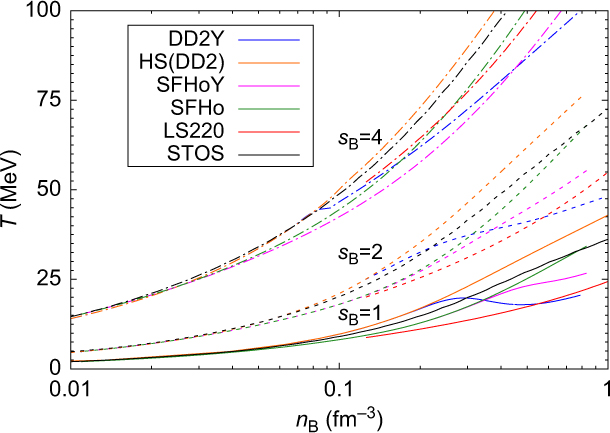
Figure 13. Same as Figure 12, but considering neutrinoless β-equilibrium instead of Y L = 0.4.
4. Summary and conclusions
Two new general purpose EoS applicable within neutron star merger and core-collapse simulations and including hyperons were proposed and discussed. The two EoS are based on the nucleonic EoS SFHo (Steiner et al. Reference Steiner, Prakash, Lattimer and Ellis2013). The entire baryonic octet is considered and the hyperonic interaction is described in the standard way for RMF models, that is, mediated by σ, ω, and ρ-mesons plus the isoscalar–vector meson with hidden strangeness φ. In one of the models the couplings of the isoscalar–vector mesons were obtained imposing SU(6) symmetry, SFHoY*, as done in most models including hyperons due to the lack of experimental information on hyperonic couplings. Since within this model the maximum mass of a cold β-equilibrated neutron star is clearly below 2 M⊙; in our second model, SFHoY, the SU(6) constraint has been relaxed and more repulsive couplings were chosen. Within the latter parameterisation, the maximum mass is compatible with the constraints imposed by the two pulsars PSR J1614-2230 (Demorest et al. Reference Demorest, Pennucci, Ransom, Roberts and Hessels2010; Fonseca et al. Reference Fonseca2016) and PSR J0348+0432 (Antoniadis et al. Reference Antoniadis2013). To determine the isoscalar–scalar hyperonic couplings, we have considered the following values for the hyperonic single particle potentials in symmetric nuclear matter:  $U_{\Lambda}^{(N)}(n_{\mathrm{sat}}) = -30$ MeV, $U_{\Sigma}^{(N)}(n_{\mathrm{sat}}) = +30$ MeV, $U_{\Xi}^{(N)}(n_{\mathrm{sat}}) = -14/-18$ MeV. We have shown, following the lines of Fortin et al. (Reference Fortin, Providencia, Raduta, Gulminelli, Zdunik, Haensel and Bejger2017), that the chosen interactions are compatible with properties of single Λ-hyperons. For future extension of our work we have indicated other parameterisations based on both the DD2 and SFHo models, which in addition allow to reproduce the bond energy of $_{\Lambda\Lambda}^6$He and to describe for two solar mass neutron stars. Our new EoS are available in tabular form from the Compose database (Typel, Oertel, & Klähn Reference Typel, Oertel and Klähn2015); see Appendix B.
The DD2Y EoS proposed in Marques et al. (Reference Lawrence, Tervala, Bedaque and Miller2017) and our new model SFHoY are the only general purpose EoS models containing the entire baryon octet up to now well compatible with the relevant constraints on the EoS. One of the main differences between these two models is the much softer symmetry energy in the underlying nuclear model SFHo than in DD2. Together with the additional repulsion needed in SFHoY to obtain a 2 M⊙ cold neutron star this leads to much lower overall hyperon fractions in SFHoY than in DD2Y. Consequently the effects on thermodynamic properties are much less pronounced in SFHoY.
In view of all above results, we may expect a different proto-neutron star evolution and an impact on neutron star merger dynamics from including hyperonic degrees of freedom within the EoS. Indications can be found from the simulations of BH formation showing a reduced time until collapse to a BH (see e.g. Peres et al. Reference Oertel, Hempel, Klähn and Typel2013) in the presence of hyperons, but further studies are required in order with EoS models, such as those presented here, allowing for all hyperons and being compatible with constraints, in particular a 2 M⊙ cold neutron star.
Author ORCIDs
Fortin M. http://orcid.org/0000-0002-9275-3733.
Acknowledgements
This work has been partially funded by the ‘Gravitation et physique fondamentale’ action of the Observatoire de Paris, by Fundação para a Ciência e Tecnologia (FCT), Portugal, under the project No. UID/FIS/04564/2016, the Polish National Science Centre (NCN) under grant No. UMO-2014/13/B/ST9/02621, and the COST action MP1304 ‘NewComsptar’.
Appendix A. Combining different parts of the EoS
The HS(DD2) and the SFHo EOS contain the transition from inhomogeneous or clusterised matter to uniform nucleonic matter. This is done via the excluded volume mechanism, which suppresses nuclei around and above nuclear saturation density. On top of that, for some thermodynamic conditions a Maxwell construction over a small range in density is necessary; for details see Hempel et al. (Reference Hempel and Schaffner-Bielich2012).
Here the situation is slightly more complicated, since homogeneous matter might contain hyperons. In the simplest case, hyperons appear within homogeneous (nucleonic) matter and it is sufficient to minimise the free energy of the homogeneous system to decide upon the particle content of matter. Such a situation occurs at low temperatures and high densities.
In some parts of the T-n B diagram, however, a transition from inhomogeneous matter directly to hyperonic homogeneous matter is observed. This is the case at low densities and high temperatures, that is, the density regions up to the bumps in Figure 6. There, light clusters compete with hyperonic degrees of freedom with only very small differences in free energy which are of the order of the numerical accuracy of the EoS calculation. From a technical point of view, in order to construct the transition in this region, we follow a similar prescription as in Banik et al. (Reference Banik, Hempel and Bandyopadhyay2014) and Marques et al. (Reference Lawrence, Tervala, Bedaque and Miller2017) and introduce a threshold value for the total hyperon fraction,  $Y_{\mathrm{hyperons}} = \sum_{j \in B_Y} n_j/n_{\rm B}$. We let hyperonic matter appear only if Y hyperons > 10−6. Note that the hyperon fraction is not the same as the strangeness fraction, Y S, defined as the sum of all particle fractions multiplied by their respective strangeness quantum numbers, $Y_{\rm S} = \sum_{j \in B} S_jn_j/n_{\rm B}$.
Although the above-described procedure allows to construct a smooth transition between the different parts of the EoS, it is of course not completely consistent. In principle, whenever hyperons compete with light nuclear clusters, the free energy of the system should be minimised allowing simultaneously for all different possibilities, for example, a coexistence of light clusters with hyperons. In view of the tiny differences in free energy and the small fractions of particles other than nucleons, electrons, and photons in the transition region, a completely consistent treatment is left for future work.
Appendix B. Technical issues of the EoS tables
The EoSs DD2Y and SFHoY are provided in a tabular form in the Compose database, http://compose.obspm.fr as a function of T, n B, Y e, either including the contribution from electrons and photons or containing only the baryonic part. Note that the Compose software allows to calculate additional quantities, such as sound speed, from those provided in the tables. Please see the Compose manual (Typel et al. Reference Typel, Röpke, Klähn, Blaschke and Wolter2015) and the data sheet on the website for more details about the definition of the different quantities.
The grid is specified as follows (with the first value in the density grid for DD2Y and the second for SFHoY and SFHoY*):

Thermodynamic quantities provided:
1. Pressure divided by baryon number density p/n B [MeV]
2. Entropy per baryon s/n B
3. Scaled baryon chemical potential μ B/mn −1
4. Scaled charge chemical potential μ Q/mn
5. Scaled (electron) lepton chemical potential μ L/mn
6. Scaled free energy per baryon f/(n Bmn)−1
7. Scaled energy per baryon e/(n Bmn)−1
Compositional data provided:
1. Particle fractions of baryons and electrons, Yi = ni/n B
2. Particle fractions of deuterons (2H), tritons (3H), 3He, and α-particles (4He)
3. Fraction of a representative (average) heavy nucleus, together with its average mass number and average charge
Please note that only non-zero particle fractions are listed.
Effective Dirac masses M* of all baryons with non-zero density are provided within homogeneous matter.