


1. Introduction
There are two key processes that influence how a galaxy evolves: star formation and black-hole accretion. The former involves the collapse of molecular gas to form stars, resulting in the build-up of stellar mass. However, such growth may be halted (typically in low-mass galaxies) if the power of supernovae is enough to expel gas from the system (Efstathiou Reference Efstathiou2000), or if gas is stripped away during interaction with another galaxy (Mihos, Richstone, & Bothun Reference Mihos, Richstone and Bothun1991) or within a cluster (Kenney et al. Reference Kenney, Geha, Jáchym, Crowl, Dague, Chung, van Gorkom and Vollmer2014). Meanwhile, material may be accreting onto the galaxy’s central, supermassive black hole. As it does so, a large amount of energy is released over a wide wavelength range (see reviews by Urry & Padovani Reference Urry and Padovani1995, Wilkes 1999 and Netzer Reference Netzer2015), and the galaxy is described as having an active galactic nucleus (AGN). AGN activity has been shown to affect the host galaxy, through both the suppression and promotion of star formation (referred to as ‘negative’ and ‘positive’ feedback, respectively). In the case of star formation being suppressed, the halo of the galaxy is heated by thermal energy from the accretion disc of the AGN, thereby preventing gas from cooling sufficiently to collapse to form stars (Croton et al. Reference Croton2006; Teyssier et al. Reference Teyssier, Moore, Martizzi, Dubois and Mayer2011). In addition, some AGN have radio jets associated with them, which may impact upon a molecular cloud, triggering its collapse and subsequent star formation (e.g. Davies et al. Reference Davies2006; Ishibashi & Fabian Reference Ishibashi and Fabian2012).
A great strength of radio observations is that they are unaffected by dust obscuration, allowing both star formation and black-hole accretion to be detected out to higher redshift than is possible at other wavelengths (e.g. Collier et al. Reference Collier2014). This includes finding high-redshift (proto-)clusters, by exploiting the tendency of ‘radio-loud’ AGN to reside in dense environments (Wylezalek et al. Reference Wylezalek2013). The added advantage of low-frequency radio data is that they allow us to select a radio source sample in an orientation-independent way. This is because the low-frequency emission of powerful AGN is dominated by the radio lobes, which are not subject to relativistic beaming (also known as ‘Doppler boosting’; Rees Reference Rees1966; Blandford & Königl Reference Blandford and KÖnigl1979). The same cannot be said for the radio core, hotspots, and jets that dominate the emission of sources at high radio frequencies. As a result of this beaming effect (which may push the observed radio brightness above the flux density limit), radio sources selected at high frequencies tend to be biased towards AGN that have their jet axis close to the line of sight.
In addition, low-frequency measurements allow us to probe older radio emission, thereby revealing a population of galaxies that had an AGN in the past but show no signs of recent activity (as verified at higher radio frequencies, e.g. Hurley-Walker et al. Reference Hurley-Walker2015). The ability to constrain the radio spectrum over a broad frequency range also exposes ‘restarted radio galaxies’, which can be used to investigate episodic jet activity (Blundell & Fabian Reference Blundell and Fabian2011; Walg et al. Reference Walg, Achterberg, Markoff, Keppens and Porth2014). This provides an idea of the timescale over which AGN activity may promote or suppress star formation in the host galaxy. Furthermore, we can use low-frequency data to uncover poorly studied processes in galaxies, such as the energetics within radio lobes. Doing so allows the internal pressure and magnetic field strengths of the lobes to be determined (e.g. Harwood et al. Reference Harwood2016). Extended frequency coverage also highlights sources with a turnover in their radio spectrum, showing that the canonical, power-law description ( $S_{\nu} \propto \nu^{\alpha}$
, with spectral index,
$S_{\nu} \propto \nu^{\alpha}$
, with spectral index,  $\alpha$
) is too simplistic for many sources (e.g. Callingham et al. Reference Callingham2017). The spectral curvature in the radio indicates that either ionised gas is present (leading to free-free absorption) or that synchrotron self-absorption is taking place (Lacki Reference Lacki2013).
$\alpha$
) is too simplistic for many sources (e.g. Callingham et al. Reference Callingham2017). The spectral curvature in the radio indicates that either ionised gas is present (leading to free-free absorption) or that synchrotron self-absorption is taking place (Lacki Reference Lacki2013).
The revised Third Cambridge Catalogue of Radio Sources (3CRR; Laing, Riley, & Longair Reference Laing, Riley and Longair1983) is currently the best-studied low-frequency radio source sample, complete with optical data. This has enabled seminal pieces of work, such as the correlation between radio jet power and optical line luminosity, found by Rawlings & Saunders (Reference Rawlings and Saunders1991). This correlation suggests that extragalactic radio sources have a common central-engine mechanism driving their emission. In addition, Barthel (Reference Barthel1989) used the 3CRR sample to show that a unification model, based on orientation of the AGN, can explain the observed properties of quasars and radio galaxies. Another example of ground-breaking work using 3CRR is that of Heckman et al. (Reference Heckman, Smith, Baum, van Breugel, Miley, Illingworth, Bothun and Balick1986), whose follow-up campaign concluded that a significant fraction of very powerful radio sources may be driven by galaxy interactions and mergers.
However, the flux density limit of 3CRR (10.9 Jy at 178 MHzFootnote a) restricts the detection of radio-loud galaxies to 173 sources. As such, there is not a sufficient number of objects for studying their cosmological evolution in detail, in terms of age or environmental density (Wang & Kaiser Reference Wang and Kaiser2008). This is a far-reaching problem, as it is thought that such sources have a significant impact in proto-clusters, through powerful jets preventing gas from cooling and falling onto proto-galaxies (Rawlings & Jarvis Reference Rawlings and Jarvis2004). This is supported by X-ray observations of clusters showing ‘cavities’ that have been carved out by radio jets (e.g. Fabian et al. Reference Fabian2000) and hydrodynamical simulations that demonstrate the effect of buoyant ‘bubbles’—inflated by the AGN—on the intracluster medium (e.g. Sijacki & Springel Reference Sijacki and Springel2006). Also, the relatively small number of high-excitation radio galaxies (HERGs; Best & Heckman Reference Best and Heckman2012) in the 3CRR sample means that how their active lifetime and jet power differs from that of low-excitation radio galaxies (LERGs) cannot be tested reliably (Turner & Shabala Reference Turner and Shabala2015). As a result, whether these properties are connected to the underlying accretion mode—thought to be different for HERGs and LERGs—requires further investigation.
AGN of similar radio flux density have been identified in the Molonglo Southern 4-Jy (MS4) Sample (Burgess & Hunstead Reference Burgess and Hunstead2006), which consists of 228 sources detected above 4 Jy at 408 MHz. The brightest of these (137 sources) form a subset that is the southern equivalent of the 3CRR sample, known as ‘SMS4’. Burgess & Hunstead (Reference Burgess and Hunstead2006) find that this subset has a greater proportion of sources larger than 5 arcmin, when compared to 3CRR, which they suggest may be due to 3CRR missing sources with low-surface-brightness. However, the 178-MHz flux densities for the SMS4 radio sources are derived through either extrapolation from or interpolation of measurements at other frequencies (namely, 80, 86, 160, 408, and 843 MHz, where available). This, therefore, complicates the comparison with 3CRR, as some of the sources may have a spectral turnover at low radio frequencies.
For this work, we use observations at low radio frequencies, obtained via the Murchison Widefield Array (MWA; Tingay et al. Reference Tingay2013). This telescope is situated in a protected radio-quiet zone, which means that there is little radio frequency interference, leading to very good spectral coverage. With 50 of the 128 antenna tiles located less than 100m from the centre of the instrument (in the original Phase-I configuration), the MWA is also sensitive to large-scale, diffuse radio emission. All-sky data have been taken through the GaLactic and Extragalactic All-sky MWA (GLEAM; Wayth et al. Reference Wayth2015) survey, and we use the ‘brightest’ detections in the EGC (Hurley-Walker et al. Reference Hurley-Walker2017) to construct the GLEAM 4-Jy (G4Jy) Sample (Jackson et al. Reference Jackson2015; White et al. Reference White2018). Our sample contains 1 863 sources and is over 10 times larger than 3CRR, due to its lower flux density limit and larger survey area. Like 3CRR, the majority of these sources are galaxies with an active black hole at the centre, and many have radio jets associated with them. By using this larger sample to study radio-bright active galaxies, we can gain a better understanding of their connection with their environment, investigate their fuelling mechanism, and more-closely analyse how these radio sources evolve over cosmic time. Furthermore, being the brightest radio sources in the southern sky makes them excellent candidates for detailed studies using the Square Kilometre Array (SKA) and its precursor/pathfinder telescopes.
However, in order to study the brightest GLEAM sources in detail, we first need to ensure that associated radio emission is collected together correctly. The necessity of this is clear for individual sources that have multiple radio detections in the GLEAM catalogue. In addition, we attempt to identify the galaxy that hosts the radio emission, so that the G4Jy Sample can be cross-matched more easily with catalogues at other wavelengths. For this, we employ visual inspection, which is the most reliable method for cross-identifying complex, extended radio sources (e.g. Williams et al. Reference Williams2019).
1.1. Paper outline
In this paper, we describe how we construct the G4Jy Sample, which consists of radio sources that are brighter than 4 Jy at 151 MHz. This involves using multi-wavelength data to collapse a list of GLEAM components into a list of GLEAM sources. Doing so is particularly important for ensuring that GLEAM flux densities incorporate all of the radio emission associated with extended sources. The resulting G4Jy catalogue includes positions for the likely host galaxy, to enable simpler cross-matching with other datasets. We also provide flux densities and angular sizes at  $\sim1\,\textrm{GHz}$
and calculate multiple sets of spectral indices.
$\sim1\,\textrm{GHz}$
and calculate multiple sets of spectral indices.
The data used for this work are summarised in Section 2, and Section 3 clarifies our initial sample selection. In Section 4, we explain how we derive brightness-weighted centroids, and our visual inspection is detailed in Section 5. Contents of the G4Jy catalogue are outlined in Section 6, with column descriptions and an excerpt of the catalogue provided in Appendix E. Sample completeness is discussed in Section 7, and initial analysis is described in Section 8. We then summarise our work in Section 9 and refer the reader to the accompanying paper (Paper II; White et al., 2020b), where we demonstrate the wide variety of bright radio sources in the G4Jy Sample and document additional literature checks.
Unless otherwise specified, we use integrated flux densities (as opposed to peak surface brightnesses) throughout this paper. In addition, we use a  $\Lambda$
CDM cosmology, with
$\Lambda$
CDM cosmology, with 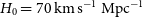 $H_{0} = 70\,\text{km\,s}^{-1}\,\text{Mpc}^{-1}$
,
$H_{0} = 70\,\text{km\,s}^{-1}\,\text{Mpc}^{-1}$
,  $\Omega_{m}=0.3$
,
$\Omega_{m}=0.3$
,  $\Omega_{\Lambda}=0.7$
. Source names that are based on B1950 coordinates are indicated via the prefix ‘B’, whilst all other position-derived names refer to J2000 coordinates. The sign convention that we use for a spectral index,
$\Omega_{\Lambda}=0.7$
. Source names that are based on B1950 coordinates are indicated via the prefix ‘B’, whilst all other position-derived names refer to J2000 coordinates. The sign convention that we use for a spectral index,  $\alpha$
, is as defined by
$\alpha$
, is as defined by  $S_{\nu} \propto \nu^{\alpha}$
.
$S_{\nu} \propto \nu^{\alpha}$
.
2. Data
The GLEAM Survey allows us to study the entire southern sky at frequencies below 300 MHz. These MWA observations provide wide spectral coverage but, in order to assess the morphology of the radio sources, we require the better spatial resolution that is afforded by other radio surveys. As such, we use data at 843 MHz, 1.4, 4.8, 8.6, and 20 GHz, which are described below, but also draw on the literature for further information (see Paper II). In addition, we collate mid-infrared and optical data for the G4Jy Sample. The former allows us to identify the likely host galaxy, including cases where the AGN is obscured by dust (e.g. Lacy et al. Reference Lacy2004). Meanwhile, optical spectra enable redshifts to be determined and provide information about the sources’ star-forming and/or AGN properties (e.g. Baldwin, Phillips, & Terlevich Reference Baldwin, Phillips and Terlevich1981; Kewley et al. Reference Kewley, Dopita, Sutherland, Heisler and Trevena2001; Sadler et al. Reference Sadler2002). Optical identifications for the G4Jy Sample will be presented in Paper III by White et al. (in preparation).
2.1. Radio data
2.1.1. GLEAM catalogue and images (72–231 MHz)
We use the EGC of the GLEAM Survey (Hurley-Walker et al. Reference Hurley-Walker2017), created using MWA observations of the southern sky (Declination,  $\delta< 30^{\circ}$
; Galactic latitude,
$\delta< 30^{\circ}$
; Galactic latitude,  $|b| >10^{\circ}$
) at low radio frequencies (72–231 MHz). The resolution of the GLEAM Survey is declination dependent and, at the central frequency of 154 MHz, is approximated by
$|b| >10^{\circ}$
) at low radio frequencies (72–231 MHz). The resolution of the GLEAM Survey is declination dependent and, at the central frequency of 154 MHz, is approximated by  $2.5 \times 2.2\,\text{arcmin}^{2}/ \cos(\delta + 26.7^{\circ})$
(Wayth et al. Reference Wayth2015). This corresponds to a typical synthesised beam of
$2.5 \times 2.2\,\text{arcmin}^{2}/ \cos(\delta + 26.7^{\circ})$
(Wayth et al. Reference Wayth2015). This corresponds to a typical synthesised beam of  $\sim2$
arcmin at 200 MHz. Twenty flux densities are measured across the 72–231 MHz band via priorised fitting, at positions determined from the ‘wide-band image’. This image was created by combining the data collected between 170 and 231 MHz, in order to achieve greater signal to noise alongside the best possible resolution. The source-finding algorithm, Aegean v1.9.6 (Hancock et al. Reference Hancock, Murphy, Gaensler, Hopkins and Curran2012; Hancock, Trott, & Hurley-Walker Reference Hancock, Trott and Hurley-Walker2018),Footnote b was performed over this image, and all Gaussian components detected above
$\sim2$
arcmin at 200 MHz. Twenty flux densities are measured across the 72–231 MHz band via priorised fitting, at positions determined from the ‘wide-band image’. This image was created by combining the data collected between 170 and 231 MHz, in order to achieve greater signal to noise alongside the best possible resolution. The source-finding algorithm, Aegean v1.9.6 (Hancock et al. Reference Hancock, Murphy, Gaensler, Hopkins and Curran2012; Hancock, Trott, & Hurley-Walker Reference Hancock, Trott and Hurley-Walker2018),Footnote b was performed over this image, and all Gaussian components detected above  $5\,\sigma$
(
$5\,\sigma$
( $S_{\textrm{200\,MHz}}\,{\gtrsim}\,$
50 mJy) were retained for the catalogue. As such, the catalogue contains 307 455 GLEAM components. In addition, we use cutouts from the wide-band image for the visual inspection described in Section 5.
$S_{\textrm{200\,MHz}}\,{\gtrsim}\,$
50 mJy) were retained for the catalogue. As such, the catalogue contains 307 455 GLEAM components. In addition, we use cutouts from the wide-band image for the visual inspection described in Section 5.
2.1.2. TGSS ADR1 catalogue and images (150 MHz)
The Giant Metrewave Radio Telescope (GMRT; Swarup 1991) previously surveyed the sky above Dec.  $=-55^{\circ}$
at 150 MHz, creating the TIFR GMRT Sky Survey (TGSS). However, due to poor data quality at low elevations, only observations at Dec.
$=-55^{\circ}$
at 150 MHz, creating the TIFR GMRT Sky Survey (TGSS). However, due to poor data quality at low elevations, only observations at Dec.  $>-53^{\circ}$
were retained for the first alternative data release (ADR1; Intema et al. Reference Intema, Jagannathan, Mooley and Frail2017), which we use for this work. In addition, Intema et al. (Reference Intema, Jagannathan, Mooley and Frail2017) note that there is incomplete coverage at
$>-53^{\circ}$
were retained for the first alternative data release (ADR1; Intema et al. Reference Intema, Jagannathan, Mooley and Frail2017), which we use for this work. In addition, Intema et al. (Reference Intema, Jagannathan, Mooley and Frail2017) note that there is incomplete coverage at  $6.5<$
R.A./h
$6.5<$
R.A./h  $<9.5$
,
$<9.5$
,  $25< \text{Dec./}^{\circ}<39$
, so we do not use TGSS data over this region. With a resolution of
$25< \text{Dec./}^{\circ}<39$
, so we do not use TGSS data over this region. With a resolution of  $25 \times 25\,\text{arcsec}^{2}$
[or
$25 \times 25\,\text{arcsec}^{2}$
[or  $25 \times 25\,\text{arcsec}^{2}/ \cos(\delta - 19^{\circ})$
for Dec.
$25 \times 25\,\text{arcsec}^{2}/ \cos(\delta - 19^{\circ})$
for Dec.  $\,{<}\,19^{\circ}$
], this survey provides useful spatial information at low frequencies, complementing the broad frequency range and surface-brightness sensitivity of the MWA. The typical rms is
$\,{<}\,19^{\circ}$
], this survey provides useful spatial information at low frequencies, complementing the broad frequency range and surface-brightness sensitivity of the MWA. The typical rms is  ${<}5\,\text{mJy\,beam}^{-1}$
(a 7-
${<}5\,\text{mJy\,beam}^{-1}$
(a 7- $\sigma$
threshold being used for the associated catalogue), and the astrometric accuracy is
$\sigma$
threshold being used for the associated catalogue), and the astrometric accuracy is  $<$
2 arcsec in R.A. and Dec. For this work, we note the flux-density scale correction found by Hurley-Walker (Reference Hurley-Walker2017) to obtain consistency between TGSS and GLEAM.
$<$
2 arcsec in R.A. and Dec. For this work, we note the flux-density scale correction found by Hurley-Walker (Reference Hurley-Walker2017) to obtain consistency between TGSS and GLEAM.
2.1.3. SUMSS catalogue and images (843 MHz)
For GLEAM components at Dec.  $<-39.5^{\circ}$
, we use images and flux densities from Version 2.1Footnote c of the Sydney University Molonglo Sky Survey (SUMSS) catalogue (Mauch et al. Reference Mauch, Murphy, Buttery, Curran, Hunstead, Piestrzynski, Robertson and Sadler2003; Murphy et al. Reference Murphy, Mauch, Green, Hunstead, Piestrzynska, Kels and Sztajer2007). This survey was conducted at a frequency of 843 MHz using the Molonglo Observatory Synthesis Telescope (Mills Reference Mills1981; Robertson Reference Robertson1991), and reaches a
$<-39.5^{\circ}$
, we use images and flux densities from Version 2.1Footnote c of the Sydney University Molonglo Sky Survey (SUMSS) catalogue (Mauch et al. Reference Mauch, Murphy, Buttery, Curran, Hunstead, Piestrzynski, Robertson and Sadler2003; Murphy et al. Reference Murphy, Mauch, Green, Hunstead, Piestrzynska, Kels and Sztajer2007). This survey was conducted at a frequency of 843 MHz using the Molonglo Observatory Synthesis Telescope (Mills Reference Mills1981; Robertson Reference Robertson1991), and reaches a  $\sim5\text{-}\sigma$
sensitivity limit of between
$\sim5\text{-}\sigma$
sensitivity limit of between  $6\,\text{mJy\,beam}^{-1}$
(Dec.
$6\,\text{mJy\,beam}^{-1}$
(Dec.  $\leq-50^{\circ}$
) and
$\leq-50^{\circ}$
) and  $10\,\text{mJy\,beam}^{-1}$
(
$10\,\text{mJy\,beam}^{-1}$
( $-50^{\circ} < $
Dec.
$-50^{\circ} < $
Dec.  $\leq -30^{\circ}$
). The resolution of these data is
$\leq -30^{\circ}$
). The resolution of these data is  $45 \times 45\ \textrm{cosec} |\delta|\,\text{arcsec}^{2}$
, and the largest positional error (
$45 \times 45\ \textrm{cosec} |\delta|\,\text{arcsec}^{2}$
, and the largest positional error ( $\sqrt{(\Delta \alpha)^{2} + (\Delta \delta)^{2}}$
, where
$\sqrt{(\Delta \alpha)^{2} + (\Delta \delta)^{2}}$
, where  $\alpha = $
Right Ascension, R.A.) is
$\alpha = $
Right Ascension, R.A.) is  $\sim30$
arcsec. However, the positional error is more typically 1–2 arcsec for sources brighter than 200 mJy at 843 MHz.
$\sim30$
arcsec. However, the positional error is more typically 1–2 arcsec for sources brighter than 200 mJy at 843 MHz.
2.1.4. NVSS catalogue and images (1.4 GHz)
The Very Large Array (VLA; Thompson et al. Reference Thompson, Clark, Wade and Napier1980) surveyed the northern sky at 1.4 GHz, down to a declination of  $-40^{\circ}$
. The resulting NRAO (National Radio Astronomy Observatory) VLA Sky Survey (NVSS; Condon et al. Reference Condon, Cotton, Greisen, Yin, Perley, Taylor and Broderick1998) has a 5-
$-40^{\circ}$
. The resulting NRAO (National Radio Astronomy Observatory) VLA Sky Survey (NVSS; Condon et al. Reference Condon, Cotton, Greisen, Yin, Perley, Taylor and Broderick1998) has a 5- $\sigma$
limit in peak source brightness of
$\sigma$
limit in peak source brightness of  $\sim2.5\,\text{mJy\,beam}^{-1}$
and a resolution of 45 arcsec. We use images and flux densities from the NVSS catalogue for GLEAM components at Dec.
$\sim2.5\,\text{mJy\,beam}^{-1}$
and a resolution of 45 arcsec. We use images and flux densities from the NVSS catalogue for GLEAM components at Dec.  $\geq-39.5^{\circ}$
, which corresponds to 77% of the G4Jy sources. The NVSS components associated with these sources are brighter than
$\geq-39.5^{\circ}$
, which corresponds to 77% of the G4Jy sources. The NVSS components associated with these sources are brighter than  $15\,\text{mJy\,beam}^{-1}$
, and so have a positional accuracy of
$15\,\text{mJy\,beam}^{-1}$
, and so have a positional accuracy of  $\lesssim$
1 arcsec.
$\lesssim$
1 arcsec.
2.1.5. The AT20G catalogue (20 GHz)
The Australia Telescope 20-GHz (AT20G) Survey (Murphy et al. Reference Murphy2010) is a blind survey over the southern sky (Dec.  $<0^{\circ}$
,
$<0^{\circ}$
,  $|b| >1.5^{\circ}$
) at 20 GHz, down to a flux density limit of 40 mJy (8
$|b| >1.5^{\circ}$
) at 20 GHz, down to a flux density limit of 40 mJy (8 $\,\sigma$
) and with a positional error of
$\,\sigma$
) and with a positional error of  $\sim1$
arcsec. The survey was conducted using the Australia Telescope Compact Array (ATCA; Frater, Brooks, & Whiteoak Reference Frater, Brooks and Whiteoak1992) and for the majority of sources below Dec. =
$\sim1$
arcsec. The survey was conducted using the Australia Telescope Compact Array (ATCA; Frater, Brooks, & Whiteoak Reference Frater, Brooks and Whiteoak1992) and for the majority of sources below Dec. =  $-15^{\circ}$
, includes near-simultaneous observations at 4.8 and 8.6 GHz (which will be used for a future paper by White et al.). As noted by Murphy et al. (Reference Murphy2010), the shortest baseline being 30.6 m limits the sensitivity of the instrument to extended emission, and so biases AT20G detections towards AGN cores and hotspots. In addition, observations at high radio frequencies (i.e. 20 GHz) are strongly affected by weather conditions. As such, the blind-scan component of the AT20G catalogue has varying completeness, ranging from 92% at
$-15^{\circ}$
, includes near-simultaneous observations at 4.8 and 8.6 GHz (which will be used for a future paper by White et al.). As noted by Murphy et al. (Reference Murphy2010), the shortest baseline being 30.6 m limits the sensitivity of the instrument to extended emission, and so biases AT20G detections towards AGN cores and hotspots. In addition, observations at high radio frequencies (i.e. 20 GHz) are strongly affected by weather conditions. As such, the blind-scan component of the AT20G catalogue has varying completeness, ranging from 92% at  $50\,\text{mJy\,beam}^{-1}$
to 98% at
$50\,\text{mJy\,beam}^{-1}$
to 98% at  $70\,\text{mJy\,beam}^{-1}$
(Hancock et al. Reference Hancock2011).
$70\,\text{mJy\,beam}^{-1}$
(Hancock et al. Reference Hancock2011).
2.2. Mid-infrared data: AllWISE catalogue and images
The Wide-field Infrared Survey Explorer (WISE; Wright et al. Reference Wright2010) has imaged the entire sky in the mid-infrared, at 3.4, 4.6, 12, and 22 $\,\mu$
m. These observing bands are referred to as W1, W2, W3, and W4 and correspond to resolutions of 6.1, 6.4, 6.5, and 12.0 arcsec, respectively. We use the AllWISE data release (Cutri et al. Reference Cutri2013), which involved combining data from the cryogenic and post-cryogenic phases of the survey. The result is improved sensitivity (0.054, 0.071, 0.73, and 5.0 mJy, respectively, at 5
$\,\mu$
m. These observing bands are referred to as W1, W2, W3, and W4 and correspond to resolutions of 6.1, 6.4, 6.5, and 12.0 arcsec, respectively. We use the AllWISE data release (Cutri et al. Reference Cutri2013), which involved combining data from the cryogenic and post-cryogenic phases of the survey. The result is improved sensitivity (0.054, 0.071, 0.73, and 5.0 mJy, respectively, at 5 $\,\sigma$
) and astrometric accuracy (
$\,\sigma$
) and astrometric accuracy ( $\ll$
1 arcsec) with respect to the WISE All-Sky data release (Cutri et al. Reference Cutri2012).
$\ll$
1 arcsec) with respect to the WISE All-Sky data release (Cutri et al. Reference Cutri2012).
2.3. Optical data: The 6dFGS catalogue
The 6-degree Field Galaxy Survey (6dFGS; Jones et al. Reference Jones2004) used the UK Schmidt Telescope (UKST; Tritton Reference Tritton1978) to obtain optical spectroscopy over the southern hemisphere (Dec.  $<0^{\circ}$
,
$<0^{\circ}$
,  $|b| >10^{\circ}$
). We use the final data release (DR3; Jones et al. Reference Jones2009), which presents redshifts for all southern sources brighter than
$|b| >10^{\circ}$
). We use the final data release (DR3; Jones et al. Reference Jones2009), which presents redshifts for all southern sources brighter than  $K=12.65$
in the 2MASS (Two Micron All Sky Survey) Extended Source Catalogue (XSC; Jarrett et al. Reference Jarrett, Chester, Cutri, Schneider, Skrutskie and Huchra2000). The resulting median redshift is 0.053.
$K=12.65$
in the 2MASS (Two Micron All Sky Survey) Extended Source Catalogue (XSC; Jarrett et al. Reference Jarrett, Chester, Cutri, Schneider, Skrutskie and Huchra2000). The resulting median redshift is 0.053.
3. Initial sample definition
Our starting point for defining the G4Jy Sample is to select all components in the GLEAM EGC (Hurley-Walker et al. Reference Hurley-Walker2017) that have an integrated flux density greater than 4 Jy at 151 MHz ( $S_{\textrm{151\,MHz}}>4\,\text{Jy}$
). This flux density limit is chosen in order to construct a sample that is over 10 times larger than the 3CRR sample, from which we can create a radio galaxy sub-sampleFootnote d that allows AGN properties to be investigated more robustly (e.g. as a function of redshift and/or environment). The resulting list of 1 879 GLEAM components is then ‘collapsed’ into a source list, where we define a source as being the object from which the radio emission originates. This is done through visual inspection (as detailed in Section 5) and is necessary as some radio sources have multiple GLEAM components. For example, a single AGN may have three entries in the GLEAM catalogue: two components marking radio lobes (where jets are interacting with the surrounding environment) and another due to an accreting ‘core’ (associated with the central supermassive black hole). Their individual flux densities can then be summed together to calculate the source’s total flux density, at each of the 20 frequencies that span the GLEAM band.
$S_{\textrm{151\,MHz}}>4\,\text{Jy}$
). This flux density limit is chosen in order to construct a sample that is over 10 times larger than the 3CRR sample, from which we can create a radio galaxy sub-sampleFootnote d that allows AGN properties to be investigated more robustly (e.g. as a function of redshift and/or environment). The resulting list of 1 879 GLEAM components is then ‘collapsed’ into a source list, where we define a source as being the object from which the radio emission originates. This is done through visual inspection (as detailed in Section 5) and is necessary as some radio sources have multiple GLEAM components. For example, a single AGN may have three entries in the GLEAM catalogue: two components marking radio lobes (where jets are interacting with the surrounding environment) and another due to an accreting ‘core’ (associated with the central supermassive black hole). Their individual flux densities can then be summed together to calculate the source’s total flux density, at each of the 20 frequencies that span the GLEAM band.
Additional GLEAM components enter the sample by association (Section 5.2), and we also search for sources that are brighter than 4 Jy but have been missed from this initial selection (Section 7). Given how the GLEAM source counts vary with flux density (Franzen et al. Reference Franzen, Vernstrom, Jackson, Hurley-Walker, Ekers, Heald, Seymour and White2019), and that visual inspection and cross-checks are very time consuming, it is currently infeasible to extend this work to a flux density limit lower than  $S_{\textrm{151\,MHz}}=4\,\text{Jy}$
. Meanwhile, concerning very bright radio sources, the following sub-section lists those that are known to be absent from the GLEAM catalogue in the first instance.
$S_{\textrm{151\,MHz}}=4\,\text{Jy}$
. Meanwhile, concerning very bright radio sources, the following sub-section lists those that are known to be absent from the GLEAM catalogue in the first instance.
3.1. Masked sources and the Orion Nebula
For readers unfamiliar with the GLEAM Survey, we clarify that the very brightest sources at Dec.  $< 30^{\circ}$
and
$< 30^{\circ}$
and  $|b| >10^{\circ}$
(belonging to a group of radio sources colloquially referred to as the ‘A-team’) are masked for the GLEAM EGC, and so do not appear in the G4Jy Sample. The sources in question are listed in Table 1 and, due to the difficulty in calibrating and imaging them at low frequencies, will be presented in a separate paper (White et al., in preparation). Also masked for the EGC are the Large and Small Magellanic Clouds, for which multi-frequency, integrated flux densities (e.g.
$|b| >10^{\circ}$
(belonging to a group of radio sources colloquially referred to as the ‘A-team’) are masked for the GLEAM EGC, and so do not appear in the G4Jy Sample. The sources in question are listed in Table 1 and, due to the difficulty in calibrating and imaging them at low frequencies, will be presented in a separate paper (White et al., in preparation). Also masked for the EGC are the Large and Small Magellanic Clouds, for which multi-frequency, integrated flux densities (e.g.  $S_{\textrm{150\,MHz}} = 1450\,\text{Jy}$
and
$S_{\textrm{150\,MHz}} = 1450\,\text{Jy}$
and  $S_{\textrm{150\,MHz}} = 258\,\text{Jy}$
, respectively) are presented by For et al. (Reference For2018). Details of the masked regions are provided in table 3 of Hurley-Walker et al. (Reference Hurley-Walker2017), with
$S_{\textrm{150\,MHz}} = 258\,\text{Jy}$
, respectively) are presented by For et al. (Reference For2018). Details of the masked regions are provided in table 3 of Hurley-Walker et al. (Reference Hurley-Walker2017), with  $<474\,\text{deg}^2$
of sky coverage being flagged due to the aforementioned sources.
$<474\,\text{deg}^2$
of sky coverage being flagged due to the aforementioned sources.
In addition, Table 1 includes the Orion Nebula (or ‘Orion A’). Although its 151-MHz flux density is well above the 4-Jy threshold (Appendix A), it was excluded by Aegean source fitting during the creation of the GLEAM catalogue. This happens when an object’s integrated flux density is more than 10 times its peak flux density, in which case the object is considered to be highly resolved, and so is removed from the catalogue. This criterion is specified because Aegean is optimised for fitting point sources and so would not provide reliable measurements for diffuse radio emission.
Table 1. A list of the brightest sources in the southern sky (Dec.  $< 30^{\circ}$
,
$< 30^{\circ}$
,  $|b| >10^{\circ}$
) that currently do not appear in the G4Jy Sample. Below, we use ‘Cen A’ as shorthand for ‘Centaurus A’. The flux densities (
$|b| >10^{\circ}$
) that currently do not appear in the G4Jy Sample. Below, we use ‘Cen A’ as shorthand for ‘Centaurus A’. The flux densities ( $S_{\textrm{151\,MHz}}$
) and spectral indices (
$S_{\textrm{151\,MHz}}$
) and spectral indices ( $\alpha$
) shown are approximate values (Hurley-Walker et al. Reference Hurley-Walker2017), based on measurements (spanning 60–1400 MHz) from the NASA/IPAC Extragalactic Database (NED)Footnote e. The exception is for *Orion A (the Orion Nebula), where these values are determined via the method described in Appendix A. Note that its spectral index is valid only very locally at 151 MHz, due to the high degree of spectral curvature.
$\alpha$
) shown are approximate values (Hurley-Walker et al. Reference Hurley-Walker2017), based on measurements (spanning 60–1400 MHz) from the NASA/IPAC Extragalactic Database (NED)Footnote e. The exception is for *Orion A (the Orion Nebula), where these values are determined via the method described in Appendix A. Note that its spectral index is valid only very locally at 151 MHz, due to the high degree of spectral curvature.
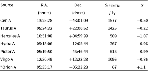
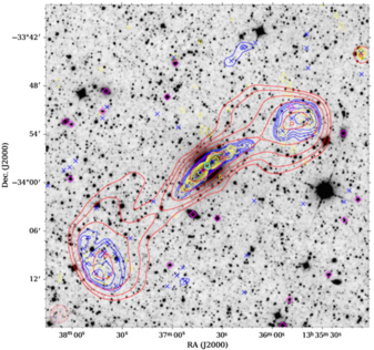
Figure 1. An overlay, centred at R.A. = 13:36:39,  $\text{Dec.} = -33:57:57$
(J2000), for an extended radio galaxy in the G4Jy Sample (G4Jy 1080, also known as IC 4296, at
$\text{Dec.} = -33:57:57$
(J2000), for an extended radio galaxy in the G4Jy Sample (G4Jy 1080, also known as IC 4296, at  $z=0.012$
). Radio contours from TGSS (150 MHz; yellow), GLEAM (170–231 MHz; red), and NVSS (1.4 GHz; blue) are overlaid on a mid-infrared image from AllWISE (
$z=0.012$
). Radio contours from TGSS (150 MHz; yellow), GLEAM (170–231 MHz; red), and NVSS (1.4 GHz; blue) are overlaid on a mid-infrared image from AllWISE ( $3.4\,\mu$
m; inverted greyscale). For each set of contours, the lowest contour is at the 3
$3.4\,\mu$
m; inverted greyscale). For each set of contours, the lowest contour is at the 3 $\,\sigma$
level (where
$\,\sigma$
level (where  $\sigma$
is the local rms), with the number of
$\sigma$
is the local rms), with the number of  $\,\sigma$
doubling with each subsequent contour (i.e. 3, 6, 12
$\,\sigma$
doubling with each subsequent contour (i.e. 3, 6, 12 $\,\sigma$
, etc.). Also plotted, in the bottom left-hand corner, are ellipses to indicate the beam sizes for TGSS (yellow with ‘+’ hatching), GLEAM (red with ‘/’ hatching), and NVSS (blue with ‘\’ hatching). This source is an unusual example, in that its GLEAM-component positions (red squares) needed to be refitted using Aegean (Hancock et al. Reference Hancock, Murphy, Gaensler, Hopkins and Curran2012; Reference Hancock, Trott and Hurley-Walker2018)—see Appendix D.1. Also plotted are catalogue positions from TGSS (yellow diamonds) and NVSS (blue crosses). The brightness-weighted centroid position, calculated using the NVSS components, is indicated by a purple hexagon. The cyan square represents an AT20G detection, marking the core of the radio galaxy. Magenta diamonds represent optical positions for sources in 6dFGS, and so we see above that G4Jy 1080 is not in this survey.
$\,\sigma$
, etc.). Also plotted, in the bottom left-hand corner, are ellipses to indicate the beam sizes for TGSS (yellow with ‘+’ hatching), GLEAM (red with ‘/’ hatching), and NVSS (blue with ‘\’ hatching). This source is an unusual example, in that its GLEAM-component positions (red squares) needed to be refitted using Aegean (Hancock et al. Reference Hancock, Murphy, Gaensler, Hopkins and Curran2012; Reference Hancock, Trott and Hurley-Walker2018)—see Appendix D.1. Also plotted are catalogue positions from TGSS (yellow diamonds) and NVSS (blue crosses). The brightness-weighted centroid position, calculated using the NVSS components, is indicated by a purple hexagon. The cyan square represents an AT20G detection, marking the core of the radio galaxy. Magenta diamonds represent optical positions for sources in 6dFGS, and so we see above that G4Jy 1080 is not in this survey.
4. Brightness-weighted centroids
The typical resolution of the MWA beamFootnote is  $\sim2$
arcmin, and so 1 785 of the final 1 863 sources (Section 6) consist of a single component in GLEAM. For the remainder, the low-frequency radio emission is so extended that it is detected as multiple GLEAM components. In order to determine which components are associated with the same ‘parent’ source, we exploit the better-resolution data afforded by the longer baselines of GMRT and higher-frequency radio surveys. Since SUMSS and NVSS offer comparable sensitivity to extended emission as GLEAM, we only consider these two datasets for this section, but supplement this with information from TGSS ADR1 in Section 5.
$\sim2$
arcmin, and so 1 785 of the final 1 863 sources (Section 6) consist of a single component in GLEAM. For the remainder, the low-frequency radio emission is so extended that it is detected as multiple GLEAM components. In order to determine which components are associated with the same ‘parent’ source, we exploit the better-resolution data afforded by the longer baselines of GMRT and higher-frequency radio surveys. Since SUMSS and NVSS offer comparable sensitivity to extended emission as GLEAM, we only consider these two datasets for this section, but supplement this with information from TGSS ADR1 in Section 5.
First, we automatically cross-correlate the 1 879 GLEAM components (Section 3) with SUMSS data at Dec  $< -39.5^{\circ}$
and with NVSS data at Dec.
$< -39.5^{\circ}$
and with NVSS data at Dec.  $\geq -39.5^{\circ}$
. This is done by using all pixels in the SUMSS/NVSS image that are within the 3-
$\geq -39.5^{\circ}$
. This is done by using all pixels in the SUMSS/NVSS image that are within the 3- $\,\sigma$
contour level, enclosing the GLEAM position being considered (and where
$\,\sigma$
contour level, enclosing the GLEAM position being considered (and where  $\sigma$
is the local rms noise in SUMSS/NVSS), to set the ‘integration area’. We then deem all catalogued SUMSS/NVSS components lying within the integration area as being associated with the GLEAM component in question. The flux densities and positions of the associated SUMSS/NVSS components are then used to calculate the brightness-weighted centroid (of the SUMSS/NVSS emission) for each GLEAM component. Based on symmetry arguments regarding the radio emission, this position therefore estimates the location of the host galaxy (i.e. the ‘parent’ source). This is useful for when we try to identify the mid-infrared position that corresponds to the G4Jy radio source (Section 5.5). For the G4Jy sources where this is not possible(/relevant), the centroid position then becomes the best reference position for cross-matching against other datasets.
$\sigma$
is the local rms noise in SUMSS/NVSS), to set the ‘integration area’. We then deem all catalogued SUMSS/NVSS components lying within the integration area as being associated with the GLEAM component in question. The flux densities and positions of the associated SUMSS/NVSS components are then used to calculate the brightness-weighted centroid (of the SUMSS/NVSS emission) for each GLEAM component. Based on symmetry arguments regarding the radio emission, this position therefore estimates the location of the host galaxy (i.e. the ‘parent’ source). This is useful for when we try to identify the mid-infrared position that corresponds to the G4Jy radio source (Section 5.5). For the G4Jy sources where this is not possible(/relevant), the centroid position then becomes the best reference position for cross-matching against other datasets.
When calculating the centroid’s positional errors in R.A. and Dec. ( $\sigma_{\alpha}$
and
$\sigma_{\alpha}$
and  $\sigma_{\delta}$
, respectively), we take a conservative approach by assuming that the positional errors of the individual SUMSS/NVSS components are correlated. If the centroid position is obtained using NVSS, we typically find that
$\sigma_{\delta}$
, respectively), we take a conservative approach by assuming that the positional errors of the individual SUMSS/NVSS components are correlated. If the centroid position is obtained using NVSS, we typically find that  $\sigma_{\alpha} \approx 0.5$
arcsec and
$\sigma_{\alpha} \approx 0.5$
arcsec and  $\sigma_{\delta} \approx 0.6$
arcsec. If the centroid position is instead obtained using SUMSS, then typically
$\sigma_{\delta} \approx 0.6$
arcsec. If the centroid position is instead obtained using SUMSS, then typically  $\sigma_{\alpha} \approx 1.5$
arcsec and
$\sigma_{\alpha} \approx 1.5$
arcsec and  $\sigma_{\delta} \approx 1.7$
arcsec. In addition, we sum the SUMSS/NVSS flux densities to obtain the total, integrated flux density at 843 MHz/1.4 GHz. For the error on the total flux density, we assume that the component flux density errors are uncorrelated, and so sum them in quadrature.
$\sigma_{\delta} \approx 1.7$
arcsec. In addition, we sum the SUMSS/NVSS flux densities to obtain the total, integrated flux density at 843 MHz/1.4 GHz. For the error on the total flux density, we assume that the component flux density errors are uncorrelated, and so sum them in quadrature.
Using this technique, SUMSS/NVSS counterparts for a GLEAM component may be missed if there is no extended emission linking them in SUMSS/NVSS. (That is, the SUMSS/NVSS components are well separated and may wrongly be assumed to be unrelated.) This can be the case for very extended radio sources. Conversely, unrelated point sources lying within the integration area of a GLEAM component will be misclassified as associated emission at 843 MHz/1.4 GHz. In order to identify and correct these errors, we visually inspect the centroid positions for each of the 1 879 GLEAM components, using overlays detailed in the next section.
5. Visual inspection
Considering the bright radio flux densities involved ( $S_{\textrm{151\,MHz}}>4\,\text{Jy}$
), it is expected that AGN dominate this sample, with many having a radio morphology that is multi-component. This poses a problem for combining radio catalogues with data at other wavelengths, where sources tend to be single component and (subject to the flux density limit) have a higher spatial density across the sky. As a result—and particularly for complex sources—a simple, nearest-neighbour cross-match will lead to incorrect association of multi-wavelength emission.
$S_{\textrm{151\,MHz}}>4\,\text{Jy}$
), it is expected that AGN dominate this sample, with many having a radio morphology that is multi-component. This poses a problem for combining radio catalogues with data at other wavelengths, where sources tend to be single component and (subject to the flux density limit) have a higher spatial density across the sky. As a result—and particularly for complex sources—a simple, nearest-neighbour cross-match will lead to incorrect association of multi-wavelength emission.
To aid the construction of multi-wavelength spectral energy distributions (SEDs) for the G4Jy Sample, we use several datasets (Section 2) for visual inspection of the selected GLEAM components. Doing so allows us to classify the morphology of the sources in question and also enables us to identify the most likely host galaxy for the radio emission. This is especially important for cases where calculation of the centroid position (Section 4) has been affected by (a) unrelated sources being blended by the NVSS/SUMSS beam (i.e. confusion); (b) unrelated—but distinct—sources in NVSS/SUMSS being incorrectly treated as ‘associated’, due to  $>3\text{-}\sigma$
emission between them; (c) the absence of extended
$>3\text{-}\sigma$
emission between them; (c) the absence of extended  $>3\text{-}\sigma$
emission linking NVSS/SUMSS components that should be associated; or (d) the radio emission not being axisymmetric [e.g. a wide-angle tail (WAT) radio galaxy, see Section 4.7 of Paper II].
$>3\text{-}\sigma$
emission linking NVSS/SUMSS components that should be associated; or (d) the radio emission not being axisymmetric [e.g. a wide-angle tail (WAT) radio galaxy, see Section 4.7 of Paper II].
By limiting this work to the brightest GLEAM components (where we have good signal-to-noise ratios), ionospheric effects and confusion noise will have little impact on our definition of the G4Jy Sample. (This is because these bright sources dominate the signal during calibration of the radio data.) In addition, the time-consuming nature of visual inspection means that we cannot justify consideration of a larger sample to a lower flux density limit (see Section 3). To this end, automated algorithms for morphology classification (e.g. ClaRAN; Wu et al. Reference Wu2019) and cross-identification will need to be developed. Until such prototype tools become proven technology, visual classification remains the most reliable method for sources with complicated morphology. In which case, an approach akin to the Radio Galaxy Zoo project (Banfield et al. Reference Banfield2015) may be needed.
5.1. Creating the overlays
We use the APLpy Python module (Robitaille & Bressert Reference Robitaille and Bressert2012) to overlay radio contours from GLEAM, TGSS, and NVSS (or SUMSS, for Dec.  $<-39.5^{\circ}$
) onto mid-infrared (W1) images from WISE (e.g. Figure 1). GLEAM images are obtained via the online GLEAM Postage Stamp Service,Footnote f whilst TGSS, NVSS, SUMSS, and WISE images are downloaded from the SkyView Virtual Observatory.Footnote g For all images, orthographic (i.e. sine) projection is used, with GLEAM images having a pixel scale of
$<-39.5^{\circ}$
) onto mid-infrared (W1) images from WISE (e.g. Figure 1). GLEAM images are obtained via the online GLEAM Postage Stamp Service,Footnote f whilst TGSS, NVSS, SUMSS, and WISE images are downloaded from the SkyView Virtual Observatory.Footnote g For all images, orthographic (i.e. sine) projection is used, with GLEAM images having a pixel scale of  $28\,\text{arcsec\,pixel}^{-1}$
. WISE images are at
$28\,\text{arcsec\,pixel}^{-1}$
. WISE images are at  $1.375\,\text{arcsec\,pixel}^{-1}$
, TGSS images are downloaded at
$1.375\,\text{arcsec\,pixel}^{-1}$
, TGSS images are downloaded at  $5\,\text{arcsec\,pixel}^{-1}$
, and a scale of
$5\,\text{arcsec\,pixel}^{-1}$
, and a scale of  $10\,\text{arcsec\,pixel}^{-1}$
is set for the NVSS and SUMSS images. For each set of radio contours, the lowest contour level that we plot is 3
$10\,\text{arcsec\,pixel}^{-1}$
is set for the NVSS and SUMSS images. For each set of radio contours, the lowest contour level that we plot is 3 $\,\sigma$
(where
$\,\sigma$
(where  $\sigma$
is the local rms).
$\sigma$
is the local rms).
The reason behind using mid-infrared images as the greyscale ‘base’ for our overlays is that this allows us to identify even the most dust-obscured host galaxies. This would not be possible if optical images were used instead. Furthermore, mid-infrared emission includes contributions from evolved stellar populations and avoids the bias of optical surveys towards actively star-forming galaxies. Of the four possible WISE bands, W1 is chosen for the imaging as this offers the best sensitivity and resolution.
Originally, our overlays were chosen to be 20 arcmin across, but first inspection of the sample revealed that a number of sources extended far beyond this size. Following a few iterations, we decided to create two sets of overlays: one set consisting of images  $1^{\circ}\ \text{across}$
(in order to encompass all of the relevant emission for the largest sources, and so more accurately classify the morphology—Section 5.2) and another set using images 10 arcmin across (acting as ‘close-ups’ for identifying the likely host galaxy—Section 5.5). For the
$1^{\circ}\ \text{across}$
(in order to encompass all of the relevant emission for the largest sources, and so more accurately classify the morphology—Section 5.2) and another set using images 10 arcmin across (acting as ‘close-ups’ for identifying the likely host galaxy—Section 5.5). For the  $1^{\circ}$
overlays, the GLEAM component’s R.A. and Dec. specifies the centre of the image. As for the 10 arcmin overlays, these are centred on the brightness-weighted centroid positions described in Section 4.
$1^{\circ}$
overlays, the GLEAM component’s R.A. and Dec. specifies the centre of the image. As for the 10 arcmin overlays, these are centred on the brightness-weighted centroid positions described in Section 4.
A problem faced when downloading images that are  $1^{\circ}$
across is that this size increases the likelihood of running into artefacts associated with poor image processing, or the source being too close to the edge of a mosaic/tile (resulting in a truncated image). Such was the case for the NVSS images of three components: GLEAM J045610
$1^{\circ}$
across is that this size increases the likelihood of running into artefacts associated with poor image processing, or the source being too close to the edge of a mosaic/tile (resulting in a truncated image). Such was the case for the NVSS images of three components: GLEAM J045610 $-$
215922, GLEAM J122039
$-$
215922, GLEAM J122039 $-$
374017, and GLEAM J154030
$-$
374017, and GLEAM J154030 $-$
051436. This was remedied by obtaining multiple images from the NVSS Postage Stamp Server,Footnote h offset in R.A. and Dec., and stitching them together using SWarp (Bertin et al. Reference Bertin, Mellier, Radovich, Missonnier, Didelon, Morin, Bohlender, Durand and Handley2002).
$-$
051436. This was remedied by obtaining multiple images from the NVSS Postage Stamp Server,Footnote h offset in R.A. and Dec., and stitching them together using SWarp (Bertin et al. Reference Bertin, Mellier, Radovich, Missonnier, Didelon, Morin, Bohlender, Durand and Handley2002).
In addition to overlaying radio contours on the mid-infrared images, we plot positions from the GLEAM, TGSS, NVSS/SUMSS, AT20G, and 6dFGS catalogues. Although AT20G is incomplete, detections from this survey indicate the presence of AGN cores, or hotspots in the radio lobes (Massardi et al. Reference Massardi2011). Meanwhile, 6dFGS positions help to identify host galaxies that are nearby/bright enough to have a spectrum from this all-sky—albeit shallow—optical survey. We also mark the centroid positions, described in the previous section, and use the errors in this position ( $\sigma_{\alpha}$
and
$\sigma_{\alpha}$
and  $\sigma_{\delta}$
) to draw an error ellipse. However, in most overlays, this ellipse is so small that it appears as a dot. Each of these datasets features in the overlay presented in Figure 1.
$\sigma_{\delta}$
) to draw an error ellipse. However, in most overlays, this ellipse is so small that it appears as a dot. Each of these datasets features in the overlay presented in Figure 1.
Both sets of overlays ( $1^{\circ}$
and 10 arcmin across), and the images from which they are made, are available online.Footnote i As the overlays are created per GLEAM component, radio sources that are multi-component will appear multiple times.
$1^{\circ}$
and 10 arcmin across), and the images from which they are made, are available online.Footnote i As the overlays are created per GLEAM component, radio sources that are multi-component will appear multiple times.
5.2. Morphological classification
As part of visually inspecting the GLEAM components, we provide a classification based on the morphology of the source in NVSS/SUMSS (and/or TGSS, where available). This classification is one of the following four categories:
‘single’—the source has a simple (typically compact) morphology in TGSS and NVSS/SUMSS;
‘double’—the source has two lobes evident in TGSS or NVSS/SUMSS, but there is no distinct detection of a core; or it has an elongated structure that is suggestive of lobes, but is accompanied by a single, catalogued detection;
‘triple’—the source has two lobes evident in TGSS or NVSS/SUMSS, and there is a distinct detection of a core in the same survey;
‘complex’—the source has a complicated morphology that does not clearly belong to any of the above categories.
When determining the morphology, we take into account extra information provided by the underlying distribution of mid-infrared sources (i.e. potential host galaxies) and the positions of AT20G detections. This helps to resolve ambiguities, particularly in cases where (for example) two nearby NVSS detections may be interpreted as either a ‘double’ radio source or two unrelated sources. For a ‘double’, we expect the host galaxy to lie about half-way between the two NVSS components, as indicated by a mid-infrared source at the centroid position. If instead there is mid-infrared emission coincident with one (or both) of the radio components, then they are likely to be unrelated. However, it can still be difficult to distinguish between a source with two radio lobes and two unrelated radio sources that are close to one another. In these situations, we consult notes by Jones & McAdam (Reference Jones and McAdam1992) on the observed structure of southern, extragalactic sources and also consider the criterion defined by Magliocchetti et al. (Reference Magliocchetti, Maddox, Lahav and Wall1998). This is where two radio components are likely to be associated if their flux densities are within a factor 4 of each other.
In addition to the morphology, for each G4Jy source, we record the following:
i. The number of NVSS/SUMSS detections associated with the radio source. The integrated flux densities for these detections are summed together to determine the total radio emission at $\sim1\,\text{GHz}$
.
$\sim1\,\text{GHz}$
.ii. The number of GLEAM components associated with the radio source. The integrated flux densities for these components are then summed together to determine the total radio emission, in each of GLEAM’s 20 sub-bands.
iii. Whether multiple sources (as judged visuallyFootnote j) contribute to the GLEAM component(s) under inspection. This acts as a ‘confusion flag’, indicating cases where the MWA beam has blended unrelated sources together.

Regarding (i), we check whether these detections match those used for the calculation of the centroid position (Section 4). In cases where there is disagreement, the centroid positions are recalculated following manual intervention. We refer to this as ‘recentroiding’ and direct the reader to Section 5.4 for further details. As for the confusion flag (iii), our criteria are that (1) unrelated sources are detected above 6 $\,\sigma$
in NVSS/SUMSS and (2) the positions of the unrelated sources’ peak emission (at
$\,\sigma$
in NVSS/SUMSS and (2) the positions of the unrelated sources’ peak emission (at  $\sim1\text{GHz}$
) are within the 3-
$\sim1\text{GHz}$
) are within the 3- $\sigma$
GLEAM contour for the G4Jy source.
$\sigma$
GLEAM contour for the G4Jy source.
We emphasise that steps (i) and (ii) above are especially important for extended sources (typically larger than 3 arcmin across), as otherwise their total radio emission may be severely underestimated. Meanwhile, step (iii) highlights cases where multiple sources contribute towards a particular detection in GLEAM. Since we are typically interested in only one of these contributing sources, the measured GLEAM flux densities will overestimate the low-frequency radio emission, and therefore must be treated with caution. In light of this, we exploit the better resolution of TGSS to judge whether the GLEAM detection crosses the  $S_{\textrm{151\,MHz}}>4\,\text{Jy}$
threshold as a consequence of confusion. However, we do not rely solely on the TGSS flux densities for this assessment, as Hurley-Walker (Reference Hurley-Walker2017) found there to be significant variation in the flux density scale over the TGSS survey area. Hence, we consider what fraction that each blended source contributes to the total emission (corresponding to the GLEAM component) at 150 MHz. If none of the blended sources has a TGSS (150 MHz) integrated flux density that corresponds to
$S_{\textrm{151\,MHz}}>4\,\text{Jy}$
threshold as a consequence of confusion. However, we do not rely solely on the TGSS flux densities for this assessment, as Hurley-Walker (Reference Hurley-Walker2017) found there to be significant variation in the flux density scale over the TGSS survey area. Hence, we consider what fraction that each blended source contributes to the total emission (corresponding to the GLEAM component) at 150 MHz. If none of the blended sources has a TGSS (150 MHz) integrated flux density that corresponds to  $S_{\textrm{151\,MHz}}>4\,\text{Jy}$
, we remove the
$S_{\textrm{151\,MHz}}>4\,\text{Jy}$
, we remove the  $S_{\textrm{151\,MHz}}>4\,\text{Jy}$
detection from the GLEAM-component list. Hence, the removal of the following components: GLEAM J093918+015948, GLEAM J101051
$S_{\textrm{151\,MHz}}>4\,\text{Jy}$
detection from the GLEAM-component list. Hence, the removal of the following components: GLEAM J093918+015948, GLEAM J101051 $-$
020137, GLEAM J201707
$-$
020137, GLEAM J201707 $-$
310305, GLEAM J202336
$-$
310305, GLEAM J202336 $-$
191144, and GLEAM J222751
$-$
191144, and GLEAM J222751 $-$
303344 (Appendix B).
$-$
303344 (Appendix B).
Meanwhile, the identification of extended low-frequency emission results in 84 components being added to the GLEAM component list by association. These are GLEAM components that individually have  $S_{\textrm{151\,MHz}}<4\,\text{Jy}$
but where visual inspection indicates that the emission should be combined with one or more other components for a particular radio source (resulting in a summed
$S_{\textrm{151\,MHz}}<4\,\text{Jy}$
but where visual inspection indicates that the emission should be combined with one or more other components for a particular radio source (resulting in a summed  $S_{\textrm{151\,MHz}}$
that is
$S_{\textrm{151\,MHz}}$
that is  $>4\,\text{Jy}$
; see also Section 7). We create individual overlays for these new components and inspect them in the same way to ensure consistency. For a list of all the sources that are multi-component in GLEAM, see Table C1 in Appendix C. The overlays for these sources are shown in Figures 1, 3–9, Appendices C and D.3, and Paper II (Figures 3–4, 6, 8, 12, 16–17, 19, 21, 23).
$>4\,\text{Jy}$
; see also Section 7). We create individual overlays for these new components and inspect them in the same way to ensure consistency. For a list of all the sources that are multi-component in GLEAM, see Table C1 in Appendix C. The overlays for these sources are shown in Figures 1, 3–9, Appendices C and D.3, and Paper II (Figures 3–4, 6, 8, 12, 16–17, 19, 21, 23).

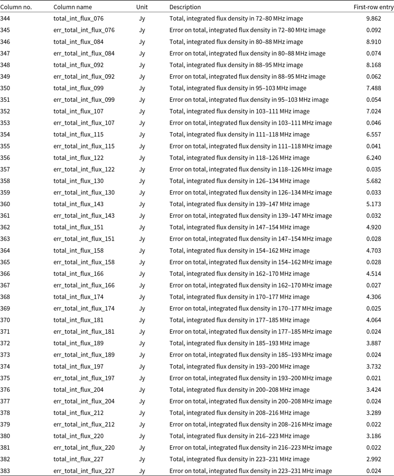
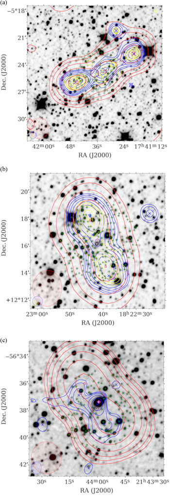
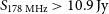
Figure 2. Examples of sources that have TGSS artefacts (Section 5.2.1), with contours, symbols, and beams as described for Figure 1. In addition, AllWISE positions (green plus signs) within 3 arcmin of the centroid position (purple hexagon) are plotted, with the host galaxy highlighted in white. (a) G4Jy 679. (b) G4Jy 938. (c) G4Jy 1005. (d) G4Jy 1085. (e) G4Jy 1209. (f) G4Jy 1239.
Table 2. 63 G4Jy sources identified as most likely having artefacts in the TGSS catalogue (Section 5.2.1).
5.2.1. Artefacts in the TGSS catalogue
Through our visual inspection, we notice that several bright radio sources (such as those in Figure 2) have low-level TGSS contours at a certain position angle ( $149.0\pm5.4^{\circ}$
and/or
$149.0\pm5.4^{\circ}$
and/or  $330.4\pm7.1^{\circ}$
) and distance from the source (
$330.4\pm7.1^{\circ}$
) and distance from the source ( $161.9\pm13.3$
arcsec).Footnote k Recognising that these are likely sidelobe artefacts, we take care not to misinterpret the morphology of the source in question (which would lead to an incorrect morphology classification). We find that these artefacts are exhibited by 63 sources (listed in Table 2), which we use to characterise the position angle and distance quoted above. However, there may be other cases where an artefact coincides with a nearby, unrelated source, making them more difficult to identify. Unfortunately, for the 63 sources considered (which have
$161.9\pm13.3$
arcsec).Footnote k Recognising that these are likely sidelobe artefacts, we take care not to misinterpret the morphology of the source in question (which would lead to an incorrect morphology classification). We find that these artefacts are exhibited by 63 sources (listed in Table 2), which we use to characterise the position angle and distance quoted above. However, there may be other cases where an artefact coincides with a nearby, unrelated source, making them more difficult to identify. Unfortunately, for the 63 sources considered (which have  $S_{\textrm{151\,MHz}}$
ranging from 4.0 to 55.9 Jy), the majority of the artefacts appear as detections in the TGSS catalogue, as indicated by yellow-diamond markers in the overlays.
$S_{\textrm{151\,MHz}}$
ranging from 4.0 to 55.9 Jy), the majority of the artefacts appear as detections in the TGSS catalogue, as indicated by yellow-diamond markers in the overlays.
5.3. Refitting with Aegean
Also connected to our visual inspection, we identify radio sources that require refitting using Aegean. This may be due to source fitting not taking into account all of the relevant emission, or the original GLEAM components appearing to have inappropriate positions (given the morphology of the radio emission). Full details regarding such sources are provided in Appendix D, where we also explain how we correct for the refitting process either under- or overestimating the integrated flux densities.
We describe the refitting as ‘unconstrained’ when it corresponds to Aegean being rerun, in its usual mode for source fitting and characterisation, over a larger region of the sky than previously. A ‘refitted flag’ of ‘1’ is used in the G4Jy catalogue to denote GLEAM components that have been refitted this way. For one source, the refitting is unconstrained but requires additional work. We use a refitting flag of ‘2’ for this scenario. In the case of ‘priorised refitting’, we constrain Aegean to use pre-determined positions for the GLEAM components. The components resulting from this type of refitting are assigned a refitting flag of ‘3’. The total number of G4Jy sources that required refitting is eight, corresponding to 15 GLEAM components. The remaining 1,945 GLEAM components, that are not refitted, retain the default flag of ‘0’.
However, we caution that Aegean may still struggle to characterise the flux density for particularly extended radio sources. This is because—like the source-fitting program, vsad (Condon et al. Reference Condon, Cotton, Greisen, Yin, Perley, Taylor and Broderick1998), used for both the NVSS and SUMSS catalogues—it fits radio components using elliptical Gaussians, and so is optimised for point sources.
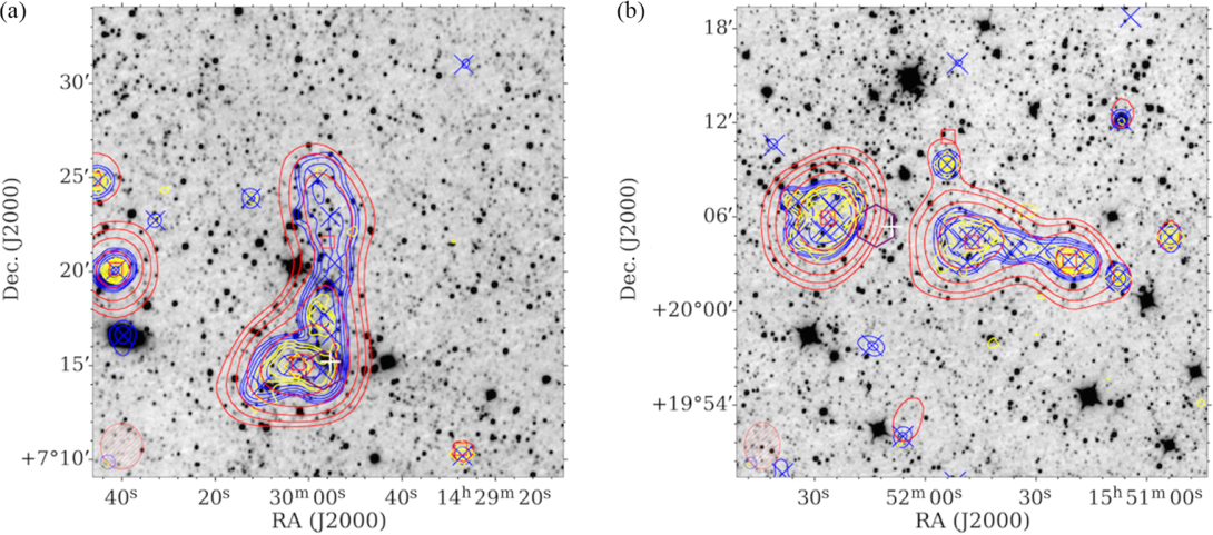
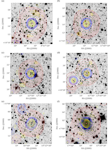
Figure 3. (a) An overlay for the source G4Jy 1173 that is centred on the component GLEAM J142955+072134. (b) An overlay for the source G4Jy 1282, centred on the component GLEAM J155147+200424. Radio contours from TGSS (150 MHz; yellow), GLEAM (170–231 MHz; red), and NVSS (1.4 GHz; blue) are overlaid on a mid-infrared image from WISE (3.4 $\mu$
m; inverted greyscale). For each set of contours, the lowest contour is at the 3
$\mu$
m; inverted greyscale). For each set of contours, the lowest contour is at the 3 $\,\sigma$
level (where
$\,\sigma$
level (where  $\sigma$
is the local rms), with the number of
$\sigma$
is the local rms), with the number of  $\sigma$
doubling with each subsequent contour (i.e. 3, 6, 12
$\sigma$
doubling with each subsequent contour (i.e. 3, 6, 12 $\,\sigma$
, etc.). As discussed in Section 5.4, manual recentroiding was required for both sources shown here, due to their complex morphology. Updated centroid positions (Section 5.4) are indicated by purple hexagons and also plotted are catalogue positions from TGSS (yellow diamonds), GLEAM (red squares), and NVSS (blue crosses).
$\,\sigma$
, etc.). As discussed in Section 5.4, manual recentroiding was required for both sources shown here, due to their complex morphology. Updated centroid positions (Section 5.4) are indicated by purple hexagons and also plotted are catalogue positions from TGSS (yellow diamonds), GLEAM (red squares), and NVSS (blue crosses).
5.4. Recentroiding after manual intervention
Following visual inspection, we find that a total of 54 sources require their brightness-weighted centroid position (Section 4) to be corrected. In the majority of cases, the error was due to incorrect association of unrelated sources, and so we specify exactly which NVSS/SUMSS components should be used when recalculating the centroid position (and integrated flux density at  $\sim1\,\text{GHz}$
). Such manual intervention is also needed for extended sources with well-separated NVSS/SUMSS components, as illustrated by G4Jy 1080 in Figure 1. (Recentroiding would usually be unnecessary for sources that are multi-component in GLEAM but have their NVSS/SUMSS components enveloped by a single 3-
$\sim1\,\text{GHz}$
). Such manual intervention is also needed for extended sources with well-separated NVSS/SUMSS components, as illustrated by G4Jy 1080 in Figure 1. (Recentroiding would usually be unnecessary for sources that are multi-component in GLEAM but have their NVSS/SUMSS components enveloped by a single 3- $\sigma$
NVSS/SUMSS contour.) The G4Jy sources, with centroids updated for these two reasons, are assigned a ‘centroid flag’ of ‘1’.
$\sigma$
NVSS/SUMSS contour.) The G4Jy sources, with centroids updated for these two reasons, are assigned a ‘centroid flag’ of ‘1’.
In addition, we note G4Jy Sources with non-axisymmetric, or very-extended, emission. Regarding the former, their morphology may be indicative of radio jets interacting with an inhomogeneous environment. Alternatively, the morphology could be the result of the galaxy’s radio jets being ‘bent backwards’ as it falls into a cluster (see Paper II). In these cases (e.g. Figure 3a), we use only the NVSS/SUMSS components that are closest to the core of the radio galaxy, as the centroid would otherwise be influenced by the geometry of the outermost regions. For extended ‘doubles’ showing evidence of multiple knots of radio emission, we also use only the innermost NVSS/SUMSS components when recalculating the centroid position. To reflect these two cases, we specify ‘2’ as the centroid flag. This is applicable for seven sources, with the updated centroid position acting as a better guide for identifying the host galaxy, as described in the next section.
Another example of association, leading to recentroiding, involves the intriguing morphology of GLEAM J155147+200424 and GLEAM J155226+200556. Both of these components have  $S_{\textrm{151\,MHz}}>4\,\text{Jy}$
, and the larger overlays created for them suggest that they are part of a single object (G4Jy 1282; Figure 3b). Indeed, this source appears as 3C 326 in the 3CRR sample (Laing et al. Reference Laing, Riley and Longair1983) and has been classified as an ‘FR II’ radio galaxy. (Such a classification is used for ‘edge-brightened’ radio galaxies, where the brightest radio emission is located in the lobes, far from the AGN (Fanaroff & Riley Reference Fanaroff and Riley1974). Other sources, where the radio luminosity decreases with distance from the AGN, are labelled ‘FR I’.) Based on this morphological interpretation, the component GLEAM J155120+200312 is added to the G4Jy Sample by association. Consequently, the NVSS components for G4Jy 1282 are redetermined manually and used for the updated centroid position.
$S_{\textrm{151\,MHz}}>4\,\text{Jy}$
, and the larger overlays created for them suggest that they are part of a single object (G4Jy 1282; Figure 3b). Indeed, this source appears as 3C 326 in the 3CRR sample (Laing et al. Reference Laing, Riley and Longair1983) and has been classified as an ‘FR II’ radio galaxy. (Such a classification is used for ‘edge-brightened’ radio galaxies, where the brightest radio emission is located in the lobes, far from the AGN (Fanaroff & Riley Reference Fanaroff and Riley1974). Other sources, where the radio luminosity decreases with distance from the AGN, are labelled ‘FR I’.) Based on this morphological interpretation, the component GLEAM J155120+200312 is added to the G4Jy Sample by association. Consequently, the NVSS components for G4Jy 1282 are redetermined manually and used for the updated centroid position.
Although Mauch et al. (Reference Mauch, Murphy, Buttery, Curran, Hunstead, Piestrzynski, Robertson and Sadler2003) invested effort into removing image artefacts from the SUMSS catalogue, we note that some still remain amongst the cutouts for the G4Jy Sample. As a result, erroneous components were being used in the centroid calculation for some sources. We rectify this by updating the centroid position, using only reliable SUMSS components (as identified via visual inspection). The affected sources are also given a centroid flag of ‘1’. The remaining 1 802 sources, which did not have their centroid position updated for any reason, retain the default centroid flag of ‘0’.
5.5. Identifying the likely host galaxy
Through topcat software (Taylor Reference Taylor, Systems, Shopbell, Britton and Ebert2005), we obtain a subset of the AllWISE catalogue, where all objects are within 3 arcmin of a centroid position belonging to the G4Jy Sample (this radius being the maximum value allowed by the ‘CDS Upload X-Match’ facility of topcat). We add these AllWISE positions (green plus signs, ‘+’) to the overlays that are 10 arcmin across and initially use a white ‘+’ to highlight the AllWISE source that is closest to the centroid position (at the centre of the overlay). We then inspect these overlays to determine whether the highlighted mid-infrared source is the likely host galaxy for the G4Jy source in question. In doing so, we also consider the errors in the centroid position (represented by an ellipse), having noted that the errors in the AllWISE positions are negligible by comparison. For 1 388 (i.e. 75%) of the 1 863 G4Jy sources, we find that the appropriate mid-infrared source has been highlighted (e.g. see Figures 2a–d, f, and 4a).
Conversely, 475 G4Jy sources require additional attention. For these radio sources, the nearest AllWISE source does not appear to be the host galaxy for the radio emission (or there is ambiguity), and so they are set aside for reinspection. This is done via interactive Multi-Catalogue Visual Cross-Matching (MCVCM) softwareFootnote l (Swan et al., in preparation), which allows us to manually select the most likely host galaxy. The corresponding 10 arcmin overlay is then updated, so that the white ‘+’ highlights this selected source (e.g. see Figures 2e and 4b–f). The result, across the 10 arcmin overlays for the full sample, is that this symbol indicates the AllWISE host galaxy identification for the G4Jy source.
Having inspected each G4Jy source, we assign a ‘host flag’ that corresponds to one of the following four categories:
‘i’—a host galaxy has been identified in the AllWISE catalogue, with the position and mid-infrared magnitudes (W1, W2, W3, W4) recorded as part of the G4Jy catalogue (Section 6),
‘u’—it is unclear which AllWISE source is the most likely host galaxy, due to the complexity of the radio morphology and/or the spatial distribution of mid-infrared sources (leading to ambiguity),
‘m’—identification of the host galaxy is limited by the mid-infrared data, with the relevant source either being too faint to be detected in AllWISE or affected by bright mid-infrared emission nearby,
‘n’—no AllWISE source should be specified, given the type of radio emission involved.
Manual identification of the host galaxy was usually required for the multi-component radio sources, where the geometry of the NVSS/SUMSS radio emission meant that the centroid position was more subject to error. In 37% of such cases, the G4Jy source had a ‘core’ indicated by a detection in 6dFGS and/or AT20G. G4Jy sources with a host galaxy in 6dFGS are noted for later analysis (Franzen et al., in preparation; White et al., in preparation), whilst those with AT20G information are explored further in a separate paper on broadband radio spectra (White et al., in preparation).
As mentioned previously, differing spatial scales of radio emission, and the fact that a single source may have multiple radio components, makes it particularly difficult to cross-match radio catalogues with data at other wavelengths (where sources typically have a singular morphology). This is complicated further by the greater density of sources seen at shorter wavelengths, leading to ambiguity when trying to identify the corresponding galaxy. Therefore, even after careful reinspection and investigation, we cannot always determine which mid-infrared source is the ‘correct’ host—hence our use of the ‘u’ flag for 129 G4Jy sources.
In some cases, we find that the radio position is robust—as suggested by the coincidence of detections from multiple radio surveys—but the likely host galaxy is too faint in the mid-infrared to appear in the AllWISE catalogue. This could be due to the radio source being at very high redshift, with confirmation of this requiring follow-up observations, such as optical/near-infrared spectroscopy (as discussed further in Section 4.10 of Paper II). For these situations (i.e. 126 G4Jy sources), we use the ‘m’ flag. However, the reader should note that this label is also used for G4Jy sources that have a bright mid-infrared host that is absent from the AllWISE catalogue, due to its photometry being affected by (for example) source confusion or a diffraction spike from a nearby star.
Our final host galaxy flag, ‘n’, is used for 2 G4Jy sources for which it is inappropriate to select a single AllWISE source, as there is no ‘host galaxy’ to identify. Such is the case for extended radio emission associated with a nebula and a cluster relic (both of which are presented in Paper II).
5.5.1. Consulting the literature
The fact that radio sources can exhibit complex and/or asymmetric morphology, coupled with the limited resolution provided by TGSS/NVSS/SUMSS (25–45 arcsec), prompts us to consult the literature as part of our host galaxy identification. For details regarding individual G4Jy sources, we refer the reader to the accompanying paper, Paper II (White et al. 2020b). Here we summarise our methods and considerations:
i. We use a mixture of radio and (candidate) mid-infrared positions to search the NED and SIMBADFootnote m databases for existing cross-identifications. For example, PKS B0503
$-$
290 and ESO 422-G028 appear as separate entries in NED, despite referring to the same source (G4Jy 517; Section 4.8 of Paper II). The only NED cross-identification that is common to both entries is ‘MSH 05
$-$
202’.ii. However, we do not ‘blindly’ use identifications from databases, but instead inspect the original images or supporting, and follow-up observations ourselves (if they are published/accessible). This allows us to corroborate (or disregard) the identification, which often involves converting between B1950 and J2000 coordinates. For example, 4.9-GHz radio contours (Massaro et al. Reference Massaro2012) lead us to question the identification for G4Jy 700 (3C 198), which dates back to Wyndham (Reference Wyndham1966). See Section 5.2 of Paper II for details.
iii. We bear in mind that many historical identifications were obtained by overlaying radio contours onto optical images, in which case they are biased against dust-obscured sources. Using our overlays (of radio contours on mid-infrared images), we consider whether there are plausible alternatives to the existing identification. If this is the case, we search for additional evidence in order to hopefully resolve the ambiguity. For example, ATCA observations in the literature confirm our host galaxy identification for G4Jy 1525 (B1910
$-$
800; see Section 7.1.1), which is in disagreement with Jones & McAdam (Reference Jones and McAdam1992).iv. For some sources, we are able to find higher-resolution (
$<$
25–45 arcsec) radio images that are presented ‘directly’ in the literature, or are available online (e.g. cutouts from FIRSTFootnote n; Faint Images of the Radio Sky at Twenty-Centimeters; White et al. Reference White, Becker, Helfand and Gregg1997). We look for evidence of the innermost part of any radio jets (if applicable) and, ideally, the radio core position. For example, FIRST reveals ‘triple’ morphology for G4Jy 367 (3C 89), allowing us to determine the correct host amongst clustered mid-infrared sources. We find this higher-resolution radio survey useful for another 20 G4Jy sources, all of which are noted individually in Paper II.v. Spectral index maps are particularly valuable for our visual checks, as we expect the radio core to be easily distinguished via its flat-spectrum emission. For example, the map provided by Safouris et al. (Reference Safouris, Subrahmanyan, Bicknell and Saripalli2009), between 1378 and 2368 MHz, confirms the radio core position for G4Jy 347 (B0319
$-$
453; Section 4.8 of Paper II), and that it is not coincident with the ‘obvious’, SUMSS-detected, mid-infrared source lying roughly midway between the two lobes.vi. Evidence of X-ray emission at the position of the host galaxy may also enable us to confirm whether or not the identification is correct. For example, Massaro et al. (Reference Massaro2012) find no detection of the putative host in the X-ray observation for G4Jy 700 (3C 198), throwing the existing identification into further doubt.
vii. For cases where the host galaxy appears to be blended, faint, or affected by artefacts in the mid-infrared, we examine optical images that are at higher resolution and may be of greater depth. For example, a SuperCOSMOS image (Hambly et al. Reference Hambly2001) suggests that two AllWISE candidates for G4Jy 1079 (Section 4.8 of Paper II) are likely a result of the host’s extended structure in the mid-infrared.
viii. Although the result is that we have fewer mid-infrared identifications in the first version of the G4Jy catalogue, our stance is to err on the side of caution until sufficient data become available.


5.5.2. Excluding possible stars
Having identified a host galaxy in the AllWISE catalogue (‘host flag’ = ‘i’) for the majority of the G4Jy sources, we subsequently check that we have not mistakenly selected a mid-infrared source that is a foreground star. We do this by first applying the following WISE-colour criteria, for separating stars from galaxies:  $[3.4]<10.5$
mag,
$[3.4]<10.5$
mag,  $[4.6]-[12]<1.5$
mag, and
$[4.6]-[12]<1.5$
mag, and  $[3.4]-[4.6] < 0.4$
mag (Jarrett et al. Reference Jarrett2011). This identifies 16 G4Jy sources for which the AllWISE source is a possible star, but reinspection confirms that either the host galaxy is unambiguous or is supported by a high-resolution radio image. If we replace the
$[3.4]-[4.6] < 0.4$
mag (Jarrett et al. Reference Jarrett2011). This identifies 16 G4Jy sources for which the AllWISE source is a possible star, but reinspection confirms that either the host galaxy is unambiguous or is supported by a high-resolution radio image. If we replace the  $[3.4]-[4.6]$
criterion with one that employs the W4 band, i.e.
$[3.4]-[4.6]$
criterion with one that employs the W4 band, i.e.  $[12] - [22]<1.2$
mag (Jarrett et al. Reference Jarrett2011), we select zero AllWISE host galaxies for reinspection. Hence, we are satisfied that none of the mid-infrared sources in the G4Jy catalogue (Section 6) are stars.
$[12] - [22]<1.2$
mag (Jarrett et al. Reference Jarrett2011), we select zero AllWISE host galaxies for reinspection. Hence, we are satisfied that none of the mid-infrared sources in the G4Jy catalogue (Section 6) are stars.
For some sources where we are uncertain as to the host galaxy identification, this may be due to obscuration by stars. This is particularly problematic for G4Jy sources at low Galactic latitude and is borne in mind during our visual inspection and checks against the literature.
For the interested reader, note that the distribution of G4Jy sources in WISE colour-colour space will be presented in Paper III, along with other multi-wavelength analysis (White et al. in preparation).
6. The GLEAM 4-Jy catalogue
This section summarises information in the G4Jy catalogue that supplements 307 columns from the parent, EGC (EGC; Hurley-Walker et al. Reference Hurley-Walker2017). For a full list of the 76 new columns that we provide, and first-row entries as examples, see Table E1 in Appendix E.
6.1. Naming of the G4Jy sources
Having identified which GLEAM components are associated with each other (Section 5) and which additional GLEAM components are to be included in the G4Jy Sample (Section 7), we sort the catalogue in order of increasing R.A. The ‘ncmp_GLEAM’ column is added to indicate the number of GLEAM components that correspond to each source. We then use simple numbering as our naming scheme: ‘G4Jy 1’, ‘G4Jy 2’, ‘G4Jy 3’, etc. This both allows a short-hand way of referring to sources and avoids ‘hard-coding’ a coordinate position that may later be refined. Similarly, we use ‘A’, ‘B’, ‘C’, etc. to label individual GLEAM components belonging to multi-component sources. For example, GLEAM J000456+124810 is the eastern radio lobe of G4Jy 7 and can be referred to as ‘G4Jy 7B’.
6.2. Morphology
The morphology of the source (Section 5.2) is determined through visual inspection and is based on NVSS/SUMSS contours, or TGSS contours where coverage allows. Although literature checks uncover radio images of higher resolution for some sources (see Paper II for details), we do not change the morphology label as we wish these to be consistent across the entire sample. Furthermore, we note that some ‘doubles’ may actually be ‘core-jet’ sources (e.g. Kellermann & Pauliny-Toth Reference Kellermann and Pauliny-Toth1981; Pearson & Readhead Reference Pearson and Readhead1988), where the radio jet emission is one-sided. However, we do not have sufficient resolution to confirm these, and so we apply Occam’s razor and leave the morphology label as ‘double’. We expect many of these morphology labels—the ‘singles’ especially—to be updated as better-resolution ( $<25$
–45 arcsec) radio images come to light.
$<25$
–45 arcsec) radio images come to light.
6.3. Information at
$\sim\textit{1}\,\text{GHz}$

The ‘Freq’ column indicates whether NVSS (1400 MHz) or SUMSS (843 MHz) has been considered for the source in question. Alongside this, we provide the number of associated NVSS/ SUMSS components (‘ncmp_NVSSorSUMSS’), the summed flux density across these components (‘S_NVSSorSUMSS’), and the brightness-weighted centroid position (‘centroid_RAJ2000’, ‘centroid_DEJ2000’) based on these components. The ‘centroid flag’ column indicates whether the centroid position is from the original, automated calculation (centroid_flag = ‘0’; see Section 4), or has been updated following manual intervention (centroid_flag = ‘1’ or ‘2’; see Section 5.4). The ‘confusion flag’ is based upon visual inspection (Section 5.2), with G4Jy sources potentially having their GLEAM flux densities affected by unrelated radio sources (confusion_flag = ‘1’; e.g. G4Jy 935 in Figure 4d) or not (confusion_flag = ‘0’; e.g. G4Jy 1628 in Figure 4f).
6.3.1. Angular sizes
We provide an estimate of the angular size at  $\sim1\,\text{GHz}$
(‘angular_size’) but warn the user that these values are only to give an indication of the extent of the radio emission. This is because the apparent size is affected by resolution (leading to overestimation) and projection (leading to underestimation). Investigating the orientation of the G4Jy sources is beyond the scope of this work, but would need to be borne in mind when using the angular sizes to estimate true, physical sizes. In addition, the angular size distribution is complicated by sources with bent-tail morphology (see Figure 3a and Section 4.7 of Paper II).
$\sim1\,\text{GHz}$
(‘angular_size’) but warn the user that these values are only to give an indication of the extent of the radio emission. This is because the apparent size is affected by resolution (leading to overestimation) and projection (leading to underestimation). Investigating the orientation of the G4Jy sources is beyond the scope of this work, but would need to be borne in mind when using the angular sizes to estimate true, physical sizes. In addition, the angular size distribution is complicated by sources with bent-tail morphology (see Figure 3a and Section 4.7 of Paper II).
For G4Jy sources that have a single component in NVSS/SUMSS, we adopt (where possible) the deconvolved major axis measurement from the respective catalogue (i.e. the MajAxis value from NVSS, or the major_axis_arcsec_afterdeconvolution value from SUMSS). For single-NVSS-component sources, we inherit the limit associated with the MajAxis value and place this in our ‘angular_size_limit’ column. Meanwhile, the SUMSS catalogue does not provide a deconvolved major axis measurement for unresolved sources. For such cases, we instead set the angular size equal to the major_axis_arcsec value—this being the original, fitted value dictated by the survey’s spatial resolution—and accompany this with angular_size_limit = ‘ $<$
’. The inequality therefore indicates which of our angular size estimates should be interpreted as upper limits. For the remaining angular sizes presented in the G4Jy catalogue, the angular_size_limit column is left blank.
$<$
’. The inequality therefore indicates which of our angular size estimates should be interpreted as upper limits. For the remaining angular sizes presented in the G4Jy catalogue, the angular_size_limit column is left blank.
For G4Jy sources that are multi-component at  $\sim1\,\text{GHz}$
, we use the largest angular separation between associated NVSS/SUMSS components as our angular size estimate (see Section 8.1 for the full-sample distribution). However, again, this value should be taken as a guide, because the fitted NVSS/SUMSS positions may not fully describe the spatial extent of the GLEAM emission. Users of the G4Jy catalogue may instead wish to consider the semi-major axis measurements output by Aegean (e.g. the a_wide and a_151 columns), but then the low spatial-resolution of GLEAM becomes an issue, as these angular sizes are not deconvolved. The reasons why we do not use TGSS positions to calculate angular sizes are that this catalogue: (i) is biased towards compact emission, (ii) does not provide coverage for all G4Jy sources, and (iii) contains artefacts around numerous bright radio sources (Section 5.2.1).
$\sim1\,\text{GHz}$
, we use the largest angular separation between associated NVSS/SUMSS components as our angular size estimate (see Section 8.1 for the full-sample distribution). However, again, this value should be taken as a guide, because the fitted NVSS/SUMSS positions may not fully describe the spatial extent of the GLEAM emission. Users of the G4Jy catalogue may instead wish to consider the semi-major axis measurements output by Aegean (e.g. the a_wide and a_151 columns), but then the low spatial-resolution of GLEAM becomes an issue, as these angular sizes are not deconvolved. The reasons why we do not use TGSS positions to calculate angular sizes are that this catalogue: (i) is biased towards compact emission, (ii) does not provide coverage for all G4Jy sources, and (iii) contains artefacts around numerous bright radio sources (Section 5.2.1).
6.4. Mid-infrared data for the host galaxies
Alongside our visual inspection (Section 5) and extensive checks against the literature (Sections 4 and 5 of Paper II), we use the ‘host_flag’ to indicate whether or not we are able to identify the host galaxy of the radio emission in the mid-infrared (Section 5.5). For G4Jy sources that are identified (host_flag = ‘i’), we provide the AllWISE name, position, and mid-infrared magnitudes (and errors) from the AllWISE catalogue. This information is being used for collating additional multi-wavelength data for the G4Jy sample and subsequent analysis (White et al., in preparation).
6.5. Total integrated GLEAM flux densities
For each of the 20 sub-band measurements provided by the GLEAM Survey, we calculate the total, integrated flux density, summed over all of the GLEAM components associated with a particular G4Jy source. The errors in these total flux densities are determined by adding in quadrature (per sub-band) the integrated flux density errors for the individual GLEAM components. If the G4Jy source is single component in GLEAM, these ‘total’ columns are simply a repeat of the integrated flux densities (and errors) for that single GLEAM component. Note that it is the total, integrated flux density at 151 MHz (‘total_int_flux_151’) that must exceed 4 Jy for a radio source to be listed in the G4Jy Sample.
Furthermore, we remind the reader that some of the individual, integrated flux densities provided in the G4Jy catalogue do not appear in the EGC. They are instead the result of refitting (and rescaling, in some cases), as described in Section 5.3 and Appendix D. We use the ‘refitted_flag’ to indicate for which GLEAM components this applies.
6.6. Four sets of spectral indices
For the majority of GLEAM components in the G4Jy Sample, the spectral index fitted over the GLEAM band (‘GLEAM_alpha’) is inherited from the EGC. In the time since the publication of Hurley-Walker et al. (Reference Hurley-Walker2017), we noticed that the spectral index errors quoted in the parent catalogue were overestimated by a factor of 5. This has been corrected in a new version of the EGC (v2), available online through VizieRFootnote o. We also include the updated error and reduced- $\chi^2$
columns in the G4Jy catalogue, renaming them ‘err_GLEAM_alpha’ and ‘reduced_chi2_GLEAM_alpha’, respectively.
$\chi^2$
columns in the G4Jy catalogue, renaming them ‘err_GLEAM_alpha’ and ‘reduced_chi2_GLEAM_alpha’, respectively.
GLEAM components that were refitted for the G4Jy catalogue (refitted_flag  $>0$
) have a newly calculated GLEAM_alpha value. For this, we fit a power-law spectrum to the integrated flux densities for multiple sub-bands, in the same way as done for GLEAM components in the EGC. Hence, we also determine consistent errors and reduced-
$>0$
) have a newly calculated GLEAM_alpha value. For this, we fit a power-law spectrum to the integrated flux densities for multiple sub-bands, in the same way as done for GLEAM components in the EGC. Hence, we also determine consistent errors and reduced- $\chi^2$
values.
$\chi^2$
values.
Table 3. The mean and median spectral index,  $\alpha$
, for each of the four sets of spectral indices provided in the G4Jy catalogue (Section 6.6). ‘Number’ refers to the number of G4Jy sources for which the statistics apply, except in the case of GLEAM_alpha, where it is the number of GLEAM components.
$\alpha$
, for each of the four sets of spectral indices provided in the G4Jy catalogue (Section 6.6). ‘Number’ refers to the number of G4Jy sources for which the statistics apply, except in the case of GLEAM_alpha, where it is the number of GLEAM components.
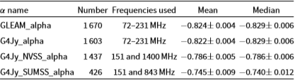
Since we are interested in the total GLEAM emission associated with each G4Jy source, we also fit a GLEAM-only spectral index using the total (i.e. summed) integrated flux densities (Section 6.5). This we refer to as ‘G4Jy_alpha’, and it will differ from GLEAM_alpha if the G4Jy source is multi-component in GLEAM. Then, in line with the parent catalogue (Hurley-Walker et al. Reference Hurley-Walker2017), we mask the GLEAM_alpha and/or G4Jy_alpha values in the G4Jy catalogue wherever the corresponding reduced- $\chi^2$
value is
$\chi^2$
value is  $>1.93$
.
$>1.93$
.
In addition, we provide the spectral index calculated using (total)  $S_{\textrm{151\,MHz}}$
and
$S_{\textrm{151\,MHz}}$
and  $S_{\textrm{1400\,MHz}}$
(‘G4Jy_NVSS_alpha’), for sources at Dec.
$S_{\textrm{1400\,MHz}}$
(‘G4Jy_NVSS_alpha’), for sources at Dec.  $\geq-39.5^{\circ}$
, and using
$\geq-39.5^{\circ}$
, and using  $S_{\textrm{151\,MHz}}$
and
$S_{\textrm{151\,MHz}}$
and  $S_{\textrm{843\,MHz}}$
(‘G4Jy_ SUMSS_alpha’), for sources at Dec.
$S_{\textrm{843\,MHz}}$
(‘G4Jy_ SUMSS_alpha’), for sources at Dec.  $<-39.5^{\circ}$
. These indices (and their errors) are provided in separate columns, as extrapolating to a common frequency (e.g. 1 GHz) may obscure the different systematics of the two surveys, and/or conflate potentially different distributions of spectral curvature.
$<-39.5^{\circ}$
. These indices (and their errors) are provided in separate columns, as extrapolating to a common frequency (e.g. 1 GHz) may obscure the different systematics of the two surveys, and/or conflate potentially different distributions of spectral curvature.
We present the mean and median values for each of these four sets of spectral indices in Table 3. Due to the masking involved for GLEAM_alpha and G4Jy_alpha, we also note the number of GLEAM components or G4Jy sources (respectively) for which the spectral index is provided in the catalogue. We direct the reader to Section 8.2 for an initial discussion of these spectral indices, with further analysis to appear in Papers III and IV (White et al., in preparation).
Table 4. Selection criteria for previous radio source samples, which we use to check the completeness of the G4Jy Sample (Section 7.1). ‘MRC’ is the abbreviation for the Molonglo Reference Catalogue of Radio Sources (Large et al. Reference Large, Mills, Little, Crawford and Sutton1981). The giant radio galaxies (GRGs) making up the sample assembled by Malarecki et al. (Reference Malarecki, Jones, Saripalli, Staveley-Smith and Subrahmanyan2015) were originally identified in the MRC ( $>\,0.7\,\text{Jy}$
at 408 MHz) and SUMSS (see Section 2.1.3).
$>\,0.7\,\text{Jy}$
at 408 MHz) and SUMSS (see Section 2.1.3).
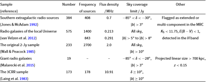
Table 5. Radio sources that were missing from the G4Jy Sample, based on the initial selection (Section 3), but are now included as a result of cross-checks against the samples listed in Table 4 (Section 7.1). Including these radio galaxies gives a total of 1 863 G4Jy sources in the sample.

12MASX J06181305-4844580 and 2ESO 509-G003 in van Velzen et al. (Reference van Velzen, Falcke, Schellart, NierstenhÖfer and Kampert2012).
7. Sample completeness
In order to do high-impact science using the G4Jy Sample and determine robust statistics on (for example) radio galaxy properties, it is crucial that the sample is complete. At this point, we note that there are two situations where we could be missing or misclassifying extended radio sources. First, our visual inspection, and subsequent investigation, may still miss very extended ‘double’ radio galaxies, where the individual lobes are separated by more than 30 arcmin. Second, and of more concern, is the possibility of missing a source that has a total flux density of  $S_{\textrm{151\,MHz}}>4\,\text{Jy}$
but is resolved into two or more components such that each component has
$S_{\textrm{151\,MHz}}>4\,\text{Jy}$
but is resolved into two or more components such that each component has  $S_{\textrm{151\,MHz}}<4\,\text{Jy}$
. These components would therefore not be included in the initial selection, using the GLEAM catalogue (Section 3). To combat this, we perform checks against numerous bright, radio source samples in the literature (Section 7.1) and also apply criteria designed to identify candidate, extended radio sources (Section 7.2). Another important factor, in terms of completeness, is the flux-density scale that we use when defining our sample at a particular frequency. This is considered in Section 7.3, before providing a brief summary of the G4Jy Sample in Section 7.4.
$S_{\textrm{151\,MHz}}<4\,\text{Jy}$
. These components would therefore not be included in the initial selection, using the GLEAM catalogue (Section 3). To combat this, we perform checks against numerous bright, radio source samples in the literature (Section 7.1) and also apply criteria designed to identify candidate, extended radio sources (Section 7.2). Another important factor, in terms of completeness, is the flux-density scale that we use when defining our sample at a particular frequency. This is considered in Section 7.3, before providing a brief summary of the G4Jy Sample in Section 7.4.
7.1. Literature searches for extended sources
We search for missing, multi-component sources by checking the overlap of the GLEAM catalogue with five existing samples: ‘Southern extragalactic radio sources’ (Jones & McAdam Reference Jones and McAdam1992), ‘Radio galaxies of the local Universe’ (van Velzen et al. Reference van Velzen, Falcke, Schellart, NierstenhÖfer and Kampert2012), the original 2-Jy sample (Wall & Peacock Reference Wall and Peacock1985), ‘Giant radio galaxies’ (Malarecki et al. Reference Malarecki, Jones, Saripalli, Staveley-Smith and Subrahmanyan2015), and the 3CRR sample (Laing et al. Reference Laing, Riley and Longair1983). An overview of these samples is shown in Table 4. The key part of this work is creating and inspecting several hundreds of extra overlays, to avoid any assumptions as to what we may expect the radio sources to look like in GLEAM.
As a result of these cross-checks, we add a total of 15 sources to the G4Jy Sample that otherwise would not have been included. However, extended sources—such as B1302 $-$
492 and B1610
$-$
492 and B1610 $-$
608 in Jones & McAdam (Reference Jones and McAdam1992)—are still absent because they lie in one of the GLEAM catalogue’s masked regions (notably, the Galactic Plane or the region surrounding Centaurus A). Therefore, we define in Section 7.4 the region over which the sample is complete.
$-$
608 in Jones & McAdam (Reference Jones and McAdam1992)—are still absent because they lie in one of the GLEAM catalogue’s masked regions (notably, the Galactic Plane or the region surrounding Centaurus A). Therefore, we define in Section 7.4 the region over which the sample is complete.
7.1.1. Cross-check using Jones & McAdam (1992)
Following the comparison with Jones & McAdam (Reference Jones and McAdam1992), we add eight sources to the G4Jy Sample: B0211 $-$
479, B0523
$-$
479, B0523 $-$
327, B0546
$-$
327, B0546 $-$
329, B1137
$-$
329, B1137 $-$
463, B1910
$-$
463, B1910 $-$
800, B2026
$-$
800, B2026 $-$
414, B2147
$-$
414, B2147 $-$
555, and B2151
$-$
555, and B2151 $-$
461 (see Table 5, and Figures 4–5). One of these is an S-shaped source (G4Jy 543; Section 4.4.2 of Paper II), another is a head-tail galaxy (G4Jy 935; Section 4.7.2 of Paper II), and another is a known GRG (G4Jy 1525; Section 4.8 of Paper II). As expected, all of the GLEAM components associated with these sources are individually
$-$
461 (see Table 5, and Figures 4–5). One of these is an S-shaped source (G4Jy 543; Section 4.4.2 of Paper II), another is a head-tail galaxy (G4Jy 935; Section 4.7.2 of Paper II), and another is a known GRG (G4Jy 1525; Section 4.8 of Paper II). As expected, all of the GLEAM components associated with these sources are individually  $< 4\,\text{Jy}$
at 151 MHz, but sum to
$< 4\,\text{Jy}$
at 151 MHz, but sum to  $>4\,\text{Jy}$
for their respective sources. In the case of B1910
$>4\,\text{Jy}$
for their respective sources. In the case of B1910 $-$
800 (the GRG, G4Jy 1525), our mid-infrared identification differs from the optical position provided by Jones & McAdam (Reference Jones and McAdam1992). Our identification of an obscured host galaxy is supported by ATCA observations of a radio core at this position (Subrahmanyan, Saripalli, & Hunstead Reference Subrahmanyan, Saripalli and Hunstead1996; Saripalli et al. Reference Saripalli, Hunstead, Subrahmanyan and Boyce2005).
$-$
800 (the GRG, G4Jy 1525), our mid-infrared identification differs from the optical position provided by Jones & McAdam (Reference Jones and McAdam1992). Our identification of an obscured host galaxy is supported by ATCA observations of a radio core at this position (Subrahmanyan, Saripalli, & Hunstead Reference Subrahmanyan, Saripalli and Hunstead1996; Saripalli et al. Reference Saripalli, Hunstead, Subrahmanyan and Boyce2005).
7.1.2. Cross-check using van Velzen et al. (2012)
Next we cross-check our sample against radio galaxies of the local Universe, as compiled by van Velzen et al. (Reference van Velzen, Falcke, Schellart, NierstenhÖfer and Kampert2012). Doing so reveals that we need to add seven sources to our sample: GIN 049, NGC 1044, GIN 190, PKS B0616 $-$
48,Footnote p B1323
$-$
48,Footnote p B1323 $-$
271, PKS B1834+19, and IC 1347 (Table 5). Six of these sources are presented in Figure 6, and we refer the reader to Figure 17 of Paper II for the seventh source. The latter is NGC 1044 (G4Jy 285), which has unusual, diffuse, low-frequency emission nearby. GIN 190 (G4Jy 475) is a head-tail galaxy (Section 4.7.2 of Paper II), and B1323
$-$
271, PKS B1834+19, and IC 1347 (Table 5). Six of these sources are presented in Figure 6, and we refer the reader to Figure 17 of Paper II for the seventh source. The latter is NGC 1044 (G4Jy 285), which has unusual, diffuse, low-frequency emission nearby. GIN 190 (G4Jy 475) is a head-tail galaxy (Section 4.7.2 of Paper II), and B1323 $-$
271 (G4Jy 1067) and PKS B1834+19 (G4Jy 1496) are both WAT radio galaxies (Section 4.7.1 of Paper II).
$-$
271 (G4Jy 1067) and PKS B1834+19 (G4Jy 1496) are both WAT radio galaxies (Section 4.7.1 of Paper II).
As part of our comparison with the catalogue produced by van Velzen et al. (Reference van Velzen, Falcke, Schellart, NierstenhÖfer and Kampert2012), we pay closer attention to sources where we significantly disagree as to the flux density measured using NVSS or SUMSS components. In Section 4.7.2 of Paper II, we detail discrepancy with respect to G4Jy 325, and we also note that for IC 4296 (G4Jy 1080 in Figure 1) they measure 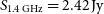 $S_{\textrm{1.4\,GHz}}=2.42\,\text{Jy}$
. This is the total flux density when summing over the NVSS components for the inner jets, but not including the NVSS components associated with the well-separated lobes. We do include the latter and calculate
$S_{\textrm{1.4\,GHz}}=2.42\,\text{Jy}$
. This is the total flux density when summing over the NVSS components for the inner jets, but not including the NVSS components associated with the well-separated lobes. We do include the latter and calculate 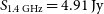 $S_{\textrm{1.4\,GHz}}=4.91\,\text{Jy}$
over 23 NVSS components.
$S_{\textrm{1.4\,GHz}}=4.91\,\text{Jy}$
over 23 NVSS components.
Comparing our NVSS/SUMSS flux densities also highlighted that we had used the wrong number of components for NGC 253 (G4Jy 86 in Figure 3a of Paper II) and NGC 612 (G4Jy 171 in Figure 7). We recalculate their flux density and brightness-weighted centroid position and duly update the centroid flags to ‘1’ (Section 5.4).
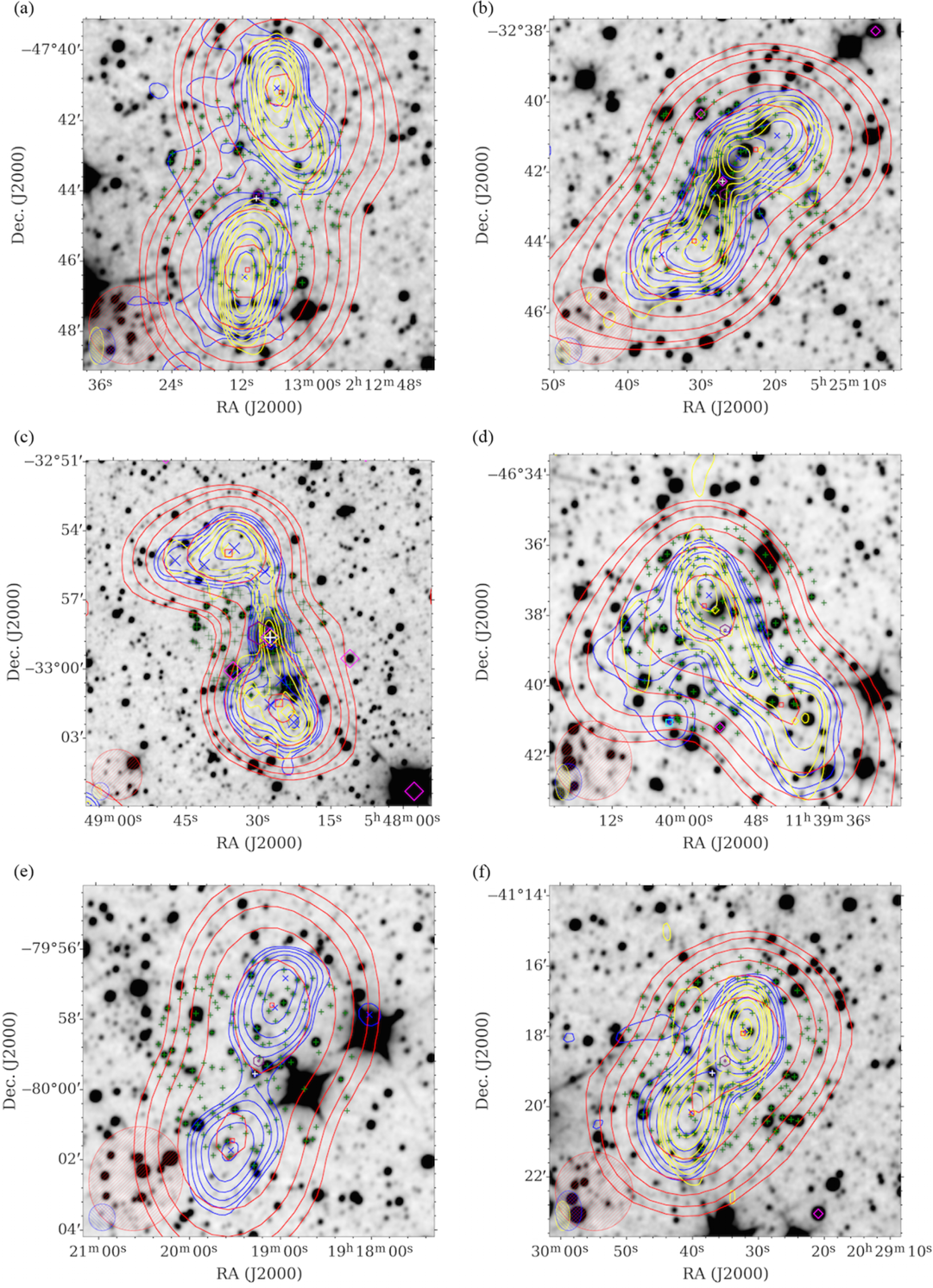
Figure 4. Overlays for six G4Jy sources that were added to the G4Jy Sample following a cross-check against Jones & McAdam (Reference Jones and McAdam1992) (Section 7.1.1). The datasets, contours, symbols, and beams are the same as those used for Figure 1, but where blue contours, crosses, and ellipses correspond to NVSS or SUMSS. In addition, positions from AllWISE are indicated by green plus signs, with host galaxies highlighted in white. (a) G4Jy 234 (B0211−479). (b) G4Jy 543 (B0523−327). (c) G4Jy 579 (B0546−329). (d) G4Jy 935 (B1137−463). (e) G4Jy 1525 (B1910−800). (f) G4Jy 1628 (B2026−414).
Table 6. A list of 3CRR sources (Laing et al. Reference Laing, Riley and Longair1983) that are not in the G4Jy Sample, despite being at Dec. $< 30^{\circ}$
. Their absence is due to each of them having poor-quality data in the GLEAM Survey, and so—with the exception of 3C 433—the region in which they lie is masked (Hurley-Walker et al. Reference Hurley-Walker2017). An explanation of why 3C 433 is present in the GLEAM catalogue, yet absent from the G4Jy Sample, can be found in Section 7.1.5. Below, we use ‘Cen A’ as shorthand for ‘Centaurus A’.
$< 30^{\circ}$
. Their absence is due to each of them having poor-quality data in the GLEAM Survey, and so—with the exception of 3C 433—the region in which they lie is masked (Hurley-Walker et al. Reference Hurley-Walker2017). An explanation of why 3C 433 is present in the GLEAM catalogue, yet absent from the G4Jy Sample, can be found in Section 7.1.5. Below, we use ‘Cen A’ as shorthand for ‘Centaurus A’.
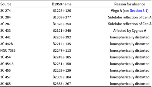
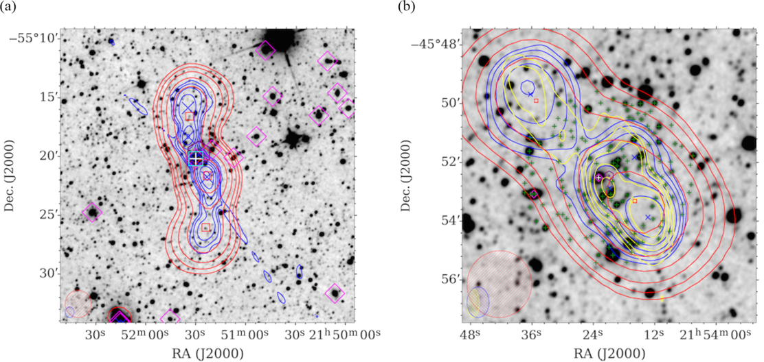
Figure 5. Overlays for two more G4Jy sources that were added to the G4Jy Sample following cross-checks against Jones & McAdam (Reference Jones and McAdam1992) (Section 7.1.1). The datasets, contours, symbols, and beams are the same as those used for Figure 4. (a) G4Jy 1732 (B2147−555). (b) G4Jy 1741 (B2151−461).
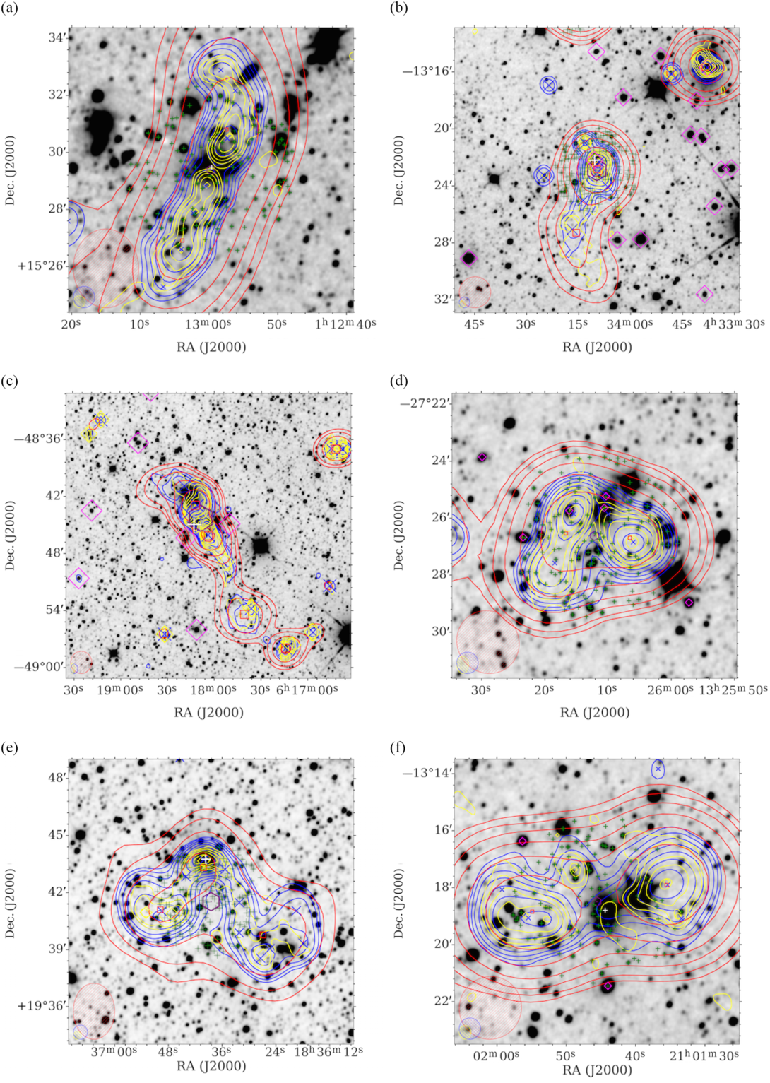
Figure 6. Overlays for six G4Jy sources that were added to the G4Jy Sample following a cross-check against van Velzen et al. (Reference van Velzen, Falcke, Schellart, NierstenhÖfer and Kampert2012) (Section 7.1.2). The datasets, contours, symbols, and beams are the same as those used for Figure 4. (a) G4Jy 131 (GIN 049). (b) G4Jy 475 (GIN 190). (c) G4Jy 604 (PKS B0616−48). (d) G4Jy 1067 (B1323−271). (e) G4Jy 1496 (PKS B1834+19). (f) G4Jy 1670 (IC 1347).
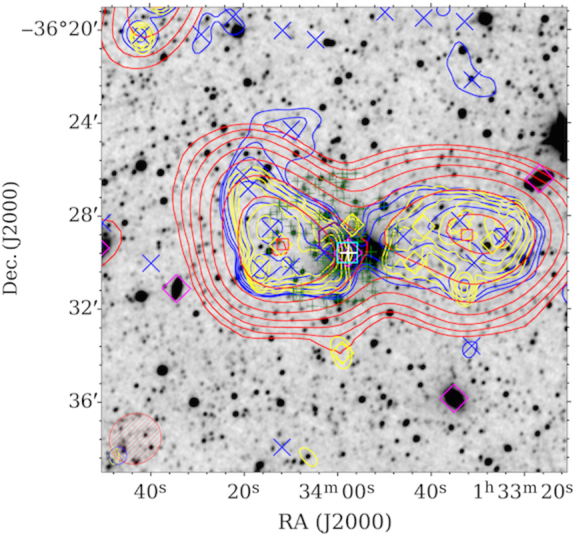
Figure 7. An overlay for G4Jy 171 (Section 7.1.2), where the datasets, contours, symbols, and beams are the same as those used for Figure 1. In addition, positions from AllWISE are indicated by green plus signs, with the host galaxy highlighted in white.
7.1.3. Cross-check using Wall & Peacock (1985)
Our cross-check against the 2-Jy sample (Wall & Peacock Reference Wall and Peacock1985) proved to be unfruitful, in terms of identifying extended radio sources that may have been missed. All radio sources found to have multiple components in GLEAM were already in the G4Jy sample via the initial selection (Section 3). This is unsurprising given that  $S_{\textrm{2.7\,GHz}}=2\,\text{Jy}$
corresponds to
$S_{\textrm{2.7\,GHz}}=2\,\text{Jy}$
corresponds to  $S_{\textrm{151\,MHz}}=15\,\text{Jy}$
, assuming a standard power-law function (
$S_{\textrm{151\,MHz}}=15\,\text{Jy}$
, assuming a standard power-law function ( $S_{\nu} \propto \nu^{\alpha}$
) with spectral index,
$S_{\nu} \propto \nu^{\alpha}$
) with spectral index,  $\alpha = -0.7$
. Nonetheless, the extra inspection was performed in case any of these bright sources showed evidence of fainter, remnant radio emission within 30 arcmin (since our larger overlays are
$\alpha = -0.7$
. Nonetheless, the extra inspection was performed in case any of these bright sources showed evidence of fainter, remnant radio emission within 30 arcmin (since our larger overlays are  $1^{\circ}\ \text{across}$
).
$1^{\circ}\ \text{across}$
).
7.1.4. Cross-check using Malarecki et al. (2015)
Our fourth cross-check is against a sample of 19 GRGs, used by Malarecki et al. (Reference Malarecki, Jones, Saripalli, Staveley-Smith and Subrahmanyan2015) to trace large-scale structure. They select this sample on the basis of proximity and size, and so these radio galaxies may be both brighter than 4 Jy and resolved into multiple GLEAM components. Upon inspection, we find that either the GRG is already in the G4Jy Sample or it has a total, integrated flux density at 151 MHz that is below the 4-Jy threshold. However, we question whether B0703–451 (G4Jy 641) is truly a GRG, due to insufficient evidence regarding its host galaxy identification (see Section 5.2 of Paper II). We also do not consider B0707–359 (G4Jy 644) to be a GRG, as its projected, linear size is  $<$
1 Mpc (instead satisfying the
$<$
1 Mpc (instead satisfying the  $>0.7\,\text{Mpc}$
criterion that Malarecki et al. Reference Malarecki, Jones, Saripalli, Staveley-Smith and Subrahmanyan2015 use to define a GRG).
$>0.7\,\text{Mpc}$
criterion that Malarecki et al. Reference Malarecki, Jones, Saripalli, Staveley-Smith and Subrahmanyan2015 use to define a GRG).
7.1.5. Cross-check using Laing et al. (1983)
Finally, we look at where the 3CRR sample (Laing et al. Reference Laing, Riley and Longair1983) overlaps with GLEAM, which corresponds to sources at  $10^{\circ}<$
Dec.
$10^{\circ}<$
Dec. $< 30^{\circ}$
. Within this declination range are 79 3CRR sources, 67 of which are already in the G4Jy Sample. These are analysed in further detail in Section 7.3. The other 12 3CRR sources, listed in Table 6, are absent from our sample due to the GLEAM data not being of sufficient quality for obtaining 20 sub-band measurements. With the exception of 3C 433 (GLEAM J212344+250412), these sources lie in masked regions of the EGC. Meanwhile, 3C 433 is not included in the G4Jy Sample because the source resides in an area of the sky (
$< 30^{\circ}$
. Within this declination range are 79 3CRR sources, 67 of which are already in the G4Jy Sample. These are analysed in further detail in Section 7.3. The other 12 3CRR sources, listed in Table 6, are absent from our sample due to the GLEAM data not being of sufficient quality for obtaining 20 sub-band measurements. With the exception of 3C 433 (GLEAM J212344+250412), these sources lie in masked regions of the EGC. Meanwhile, 3C 433 is not included in the G4Jy Sample because the source resides in an area of the sky ( $-18.3^{\circ} < b < -10.0^{\circ}$
,
$-18.3^{\circ} < b < -10.0^{\circ}$
,  $65.4^{\circ} < l < 81.1^{\circ}$
, Dec.
$65.4^{\circ} < l < 81.1^{\circ}$
, Dec. $<30.0^{\circ}$
) that is difficult to calibrate, due to the influence of Cygnus A [at R.A. = 19:59:28.36, Dec. = +40:44:02.1 (J2000)]. Although the rms noise is too high for the point spread function to be characterised at each of GLEAM’s 20 sub-bands, the noise in the wide-band image (170–231 MHz) is sufficiently low for wide-band measurements (and the source-fitting that follows). Hence, the GLEAM catalogue contains 363 components in this region that have wide-band flux densities but no sub-band flux densities (plus another 7 components with negative-value
$<30.0^{\circ}$
) that is difficult to calibrate, due to the influence of Cygnus A [at R.A. = 19:59:28.36, Dec. = +40:44:02.1 (J2000)]. Although the rms noise is too high for the point spread function to be characterised at each of GLEAM’s 20 sub-bands, the noise in the wide-band image (170–231 MHz) is sufficiently low for wide-band measurements (and the source-fitting that follows). Hence, the GLEAM catalogue contains 363 components in this region that have wide-band flux densities but no sub-band flux densities (plus another 7 components with negative-value  $S_{\textrm{151\,MHz}}$
). This means that there may be additional sources brighter than 4 Jy at 151 MHz (our sub-band of interest). We take this into account (in Section 7.4) by considering our completeness over the EGC footprint minus the region defined above.
$S_{\textrm{151\,MHz}}$
). This means that there may be additional sources brighter than 4 Jy at 151 MHz (our sub-band of interest). We take this into account (in Section 7.4) by considering our completeness over the EGC footprint minus the region defined above.
7.2. Internal matching of the EGC
We also search for missing sources by cross-matching the GLEAM components into pairs/groups and then selecting potential, extended G4Jy sources for visual inspection. The two methods we use for selecting these candidate sources are described below. Following inspection of internal matches, we add a total of nine sources to the G4Jy Sample that would otherwise be absent.
7.2.1. Applying a 4-arcmin matching radius
For the first method, we use topcat to apply a friend-of-friends internal match, which is based purely on GLEAM positions. This allows us to include ‘chains’ of low-frequency radio emission in our selection, and we set 4 arcmin as the maximum separation between two adjacent GLEAM components. This matching radius is chosen bearing in mind the resolution of GLEAM ( $\sim2$
arcmin), and that if the GLEAM components are well-separated, it becomes more difficult to tell whether the radio emission is associated or not. Furthermore, a 1-Mpc source at
$\sim2$
arcmin), and that if the GLEAM components are well-separated, it becomes more difficult to tell whether the radio emission is associated or not. Furthermore, a 1-Mpc source at  $z\sim0.5$
is
$z\sim0.5$
is  $<$
3 arcmin in angular size, and we do not expect an overabundance of GRGs at low redshift.
$<$
3 arcmin in angular size, and we do not expect an overabundance of GRGs at low redshift.
After removing groups with at least one GLEAM component brighter than 4 Jy (since these have already been inspected), there remains 14441 groupings. We then sum  $S_{\textrm{151\,MHz}}$
for each group and retain those for which the total is
$S_{\textrm{151\,MHz}}$
for each group and retain those for which the total is  $>4\,\text{Jy}$
. This drastically cuts the number of GLEAM components down to 88. A further 10 are removed, as they have already been identified as belonging to the G4Jy Sample via our cross-checks against the literature (Section 7.1). For the remaining 78 GLEAM components (forming 37 groups), we download the relevant images and create new overlays for visual inspection. We find that the majority of these groups are the result of unrelated GLEAM components being close to one another, whilst the remainder are groups that genuinely represent associated low-frequency emission. This prompts us to add another nine radio galaxies to the G4Jy Sample, which are listed in Table 7 and presented in Figures 8–9. Of particular note is the S-shaped source, G4Jy 447 (Section 4.4.2 of Paper II).
$>4\,\text{Jy}$
. This drastically cuts the number of GLEAM components down to 88. A further 10 are removed, as they have already been identified as belonging to the G4Jy Sample via our cross-checks against the literature (Section 7.1). For the remaining 78 GLEAM components (forming 37 groups), we download the relevant images and create new overlays for visual inspection. We find that the majority of these groups are the result of unrelated GLEAM components being close to one another, whilst the remainder are groups that genuinely represent associated low-frequency emission. This prompts us to add another nine radio galaxies to the G4Jy Sample, which are listed in Table 7 and presented in Figures 8–9. Of particular note is the S-shaped source, G4Jy 447 (Section 4.4.2 of Paper II).
Consideration of a tenth source for the sample was more convoluted but, ultimately, short lived. This NVSS ‘triple’ is blended with an unrelated point source, together having their low-frequency emission characterised by GLEAM J215506–321945 and GLEAM J215519–321841. The relative TGSS flux densities of the two sources suggest that the ‘triple’ exceeds the 4-Jy threshold (cf. Appendix B), so we attempted to de-blend their GLEAM emission via priorised refitting (cf. Appendix D.3). However, the refitted  $S_{\textrm{151\,MHz}}$
for the ‘triple’ is below 4 Jy, and so the source is not considered any further.
$S_{\textrm{151\,MHz}}$
for the ‘triple’ is below 4 Jy, and so the source is not considered any further.
7.2.2. Applying empirically derived criteria
For our second method, we use two criteria: a flux density ratio of  $0.5<S_{1}/S_{2}< 2$
and a normalised separation (in degrees/
$0.5<S_{1}/S_{2}< 2$
and a normalised separation (in degrees/ $\sqrt{\textrm{Jy}}$
) of
$\sqrt{\textrm{Jy}}$
) of 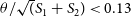 $\theta/\sqrt(S_{1}+S_{2})<0.13$
, where
$\theta/\sqrt(S_{1}+S_{2})<0.13$
, where  $S_{1}$
and
$S_{1}$
and  $S_{2}$
are the 151 MHz flux densities in Jy. This parameter space was chosen from examination of flux density ratio plotted against normalised separation, for sources from the FIRST survey (White et al. Reference White, Becker, Helfand and Gregg1997). That analysis has been done as part of the follow-up to an automated cross-identification paper based on the likelihood ratio (lrpy; Weston et al. Reference Weston, Seymour, Gulyaev, Norris, Banfield, Vaccari, Hopkins and Franzen2018). The goal was to select pairs of radio components that could potentially be true ‘doubles’ and then see whether the lrpy code would be more likely to select a counterpart to the radio source if it was a ‘double’, compared to if it were two ‘single’ sources. The normalised separation comes from the assumption that the luminosity is constant and therefore distance is proportional to
$S_{2}$
are the 151 MHz flux densities in Jy. This parameter space was chosen from examination of flux density ratio plotted against normalised separation, for sources from the FIRST survey (White et al. Reference White, Becker, Helfand and Gregg1997). That analysis has been done as part of the follow-up to an automated cross-identification paper based on the likelihood ratio (lrpy; Weston et al. Reference Weston, Seymour, Gulyaev, Norris, Banfield, Vaccari, Hopkins and Franzen2018). The goal was to select pairs of radio components that could potentially be true ‘doubles’ and then see whether the lrpy code would be more likely to select a counterpart to the radio source if it was a ‘double’, compared to if it were two ‘single’ sources. The normalised separation comes from the assumption that the luminosity is constant and therefore distance is proportional to  $1/\sqrt S$
, and that the linear size is also constant. Neither of these assumptions is true, but we note that when plotting these parameters against each other using FIRST, there is a cloud of sources within the region bound by the two criteria, as well as a larger (partially overlapping) distribution. The cloud of sources most likely corresponds to true pairs (i.e. the two lobes of one radio source), and the more widespread distribution (going to higher flux density ratios and normalised separations) is due to random matches. This separation of ‘true pairs’ and ‘random pairs’ is confirmed by visual inspection of a randomly selected sub-sample. We note that this parameter space happens to be equivalent to that from Magliocchetti et al. (Reference Magliocchetti, Maddox, Lahav and Wall1998), albeit derived differently.
$1/\sqrt S$
, and that the linear size is also constant. Neither of these assumptions is true, but we note that when plotting these parameters against each other using FIRST, there is a cloud of sources within the region bound by the two criteria, as well as a larger (partially overlapping) distribution. The cloud of sources most likely corresponds to true pairs (i.e. the two lobes of one radio source), and the more widespread distribution (going to higher flux density ratios and normalised separations) is due to random matches. This separation of ‘true pairs’ and ‘random pairs’ is confirmed by visual inspection of a randomly selected sub-sample. We note that this parameter space happens to be equivalent to that from Magliocchetti et al. (Reference Magliocchetti, Maddox, Lahav and Wall1998), albeit derived differently.
Through this analysis we find 47 potential ‘doubles’ where both GLEAM components are brighter than 4 Jy. Of these, 18 are confirmed through visual inspection to be true ‘doubles’, and one is a ‘triple’. (All 19 had already been identified as multi-GLEAM-component sources.) The remaining 28 candidate ‘doubles’ are found to be pairs of GLEAM components that are not associated with one another. Furthermore, there are 14 other previously confirmed ‘doubles’/‘triples’ (Section 5.2) that are not selected via the criteria above. Therefore, for this subset ( $S_{1}$
,
$S_{1}$
,  $S_{2}>4\,\text{Jy}$
), we estimate the reliability of the algorithm as
$S_{2}>4\,\text{Jy}$
), we estimate the reliability of the algorithm as  $19/47=0.40$
, and its completeness as
$19/47=0.40$
, and its completeness as  $19/33=0.58$
.
$19/33=0.58$
.
Table 7. Radio sources that are now included in the G4Jy Sample, having been identified through a friends-of-friends match using the GLEAM EGC (Section 7.2.1). Including these radio galaxies gives a total of 1 863 G4Jy sources in the sample.
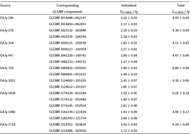
Meanwhile, out of eight potential ‘doubles’ where both GLEAM components are fainter than 4 Jy, we find that one of them is a true ‘double’ with total flux density  $>4\,$
Jy. This is G4Jy 729 (Figure 8e), which was found via our previous method (Section 7.2.1). That method led to us identifying eight other radio galaxies, but none of these are selected via the criteria based on flux density ratio and normalised separation. Hence, for this subset (
$>4\,$
Jy. This is G4Jy 729 (Figure 8e), which was found via our previous method (Section 7.2.1). That method led to us identifying eight other radio galaxies, but none of these are selected via the criteria based on flux density ratio and normalised separation. Hence, for this subset ( $S_{1}$
,
$S_{1}$
,  $S_{2}<4\,\text{Jy}$
;
$S_{2}<4\,\text{Jy}$
;  $S_{1}+S_{2}>4\,\text{Jy}$
), we estimate the reliability of the algorithm as
$S_{1}+S_{2}>4\,\text{Jy}$
), we estimate the reliability of the algorithm as  $1/8=0.13$
and its completeness as
$1/8=0.13$
and its completeness as  $1/9=0.11$
.
$1/9=0.11$
.
The main reason why applying this method to GLEAM data did not work very well (considering the reliability and completeness) is likely that the selection criteria were derived for radio sources in FIRST. Radio galaxy populations from this survey are incomplete and biased towards sources with their radio axis close to our line of sight. Furthermore, FIRST is sensitive to bright, compact emission, and so would pick up a greater proportion of radio galaxies that have distinct hotspots (typical of ‘double’, FR-II morphology). In GLEAM, we see radio sources with more diffuse emission and a wider range of morphology, for which the selection criteria are less appropriate. However, this method was able to select very extended radio sources with GLEAM-component separations,  $\theta'$
, of up to 8 arcmin. Those with separations of
$\theta'$
, of up to 8 arcmin. Those with separations of  $\theta' < 4'$
(11 sources) would have been selected for visual inspection via the approach taken in Section 7.2.1, while the remaining nine sources (with
$\theta' < 4'$
(11 sources) would have been selected for visual inspection via the approach taken in Section 7.2.1, while the remaining nine sources (with  $4' < \theta' < 8'$
) would not have been. Nonetheless, the latter subset each have at least one GLEAM component with
$4' < \theta' < 8'$
) would not have been. Nonetheless, the latter subset each have at least one GLEAM component with  $S_{\textrm{151\,MHz}}>4\,\text{Jy}$
, and so were already visually inspected following the initial selection (Section 3).
$S_{\textrm{151\,MHz}}>4\,\text{Jy}$
, and so were already visually inspected following the initial selection (Section 3).
Figure 8. Overlays for six G4Jy sources that were added to the G4Jy Sample following internal matching (Section 7.2.1). The datasets, contours, symbols, and beams are the same as those used for Figure 4. (a) G4Jy 189. (b) G4Jy 270. (c) G4Jy 318. (d) G4Jy 447. (e) G4Jy 729. (f) G4Jy 1021.

Figure 9. Overlays for three more G4Jy sources that were added to the G4Jy Sample following internal matching (Section 7.2.1). Datasets, contours, symbols, and beams are the same as for Figure 4. (a) G4Jy 1428. (b) G4Jy 1480. (c) G4Jy 1718.
Table 8. The 67 G4Jy sources that are also in the 3CRR sample. ‘No. comp.’ refers to the number of GLEAM components associated with the G4Jy source, and ‘3CRR ref.’ indicates the origin of the 3CRR 178-MHz flux density: 1—4CT (Williams et al. Reference Williams, Collins, Caswell and Holden1968; Caswell & Crowther Reference Caswell and Crowther1969; Kellermann et al. Reference Kellermann, Pauliny-Toth and Williams1969); 2—4C (Clarke Reference Clarke1965; Wills & Parker Reference Wills and Parker1966); 3—4C (Pilkington & Scott Reference Pilkington and Scott1965; Gower, Scott, & Wills Reference Gower, Scott and Wills1967); 4—3CR (Bennett Reference Bennett1962); 5—corrected 3CR (Véron Reference VÉron1977); 6—interpolation or extrapolation. The references provide expressions for the corresponding beamsize, which we evaluate at the relevant declination, and present in the next column. These ‘3CRR beams’ are applied to GLEAM images (Section 7.3), from which we derive the  $S_{\textrm{178\,MHz}}$
shown in column 7.
$S_{\textrm{178\,MHz}}$
shown in column 7.  $S_{\textrm{178\,MHz}}$
values in column 8 are calculated by extrapolating from 181 MHz to 178 MHz using the G4Jy_alpha value (Section 6.6), or the spectral index from the 3CRR catalogue (as indicated by ‘
$S_{\textrm{178\,MHz}}$
values in column 8 are calculated by extrapolating from 181 MHz to 178 MHz using the G4Jy_alpha value (Section 6.6), or the spectral index from the 3CRR catalogue (as indicated by ‘ $\alpha$
flag’ = 1). Due to space considerations, we note here that columns 4, 7, and 8 are in units of Jy. The ‘original ratio’ is the extrapolated, GLEAM
$\alpha$
flag’ = 1). Due to space considerations, we note here that columns 4, 7, and 8 are in units of Jy. The ‘original ratio’ is the extrapolated, GLEAM  $S_{\textrm{178\,MHz}}$
(column 8) divided by the 3CRR
$S_{\textrm{178\,MHz}}$
(column 8) divided by the 3CRR  $S_{\textrm{178\,MHz}}$
. For the ‘rescaled ratio’ we instead divide by a rescaled version of the 3CRR
$S_{\textrm{178\,MHz}}$
. For the ‘rescaled ratio’ we instead divide by a rescaled version of the 3CRR  $S_{\textrm{178\,MHz}}$
, as described in Section 7.3.
$S_{\textrm{178\,MHz}}$
, as described in Section 7.3.
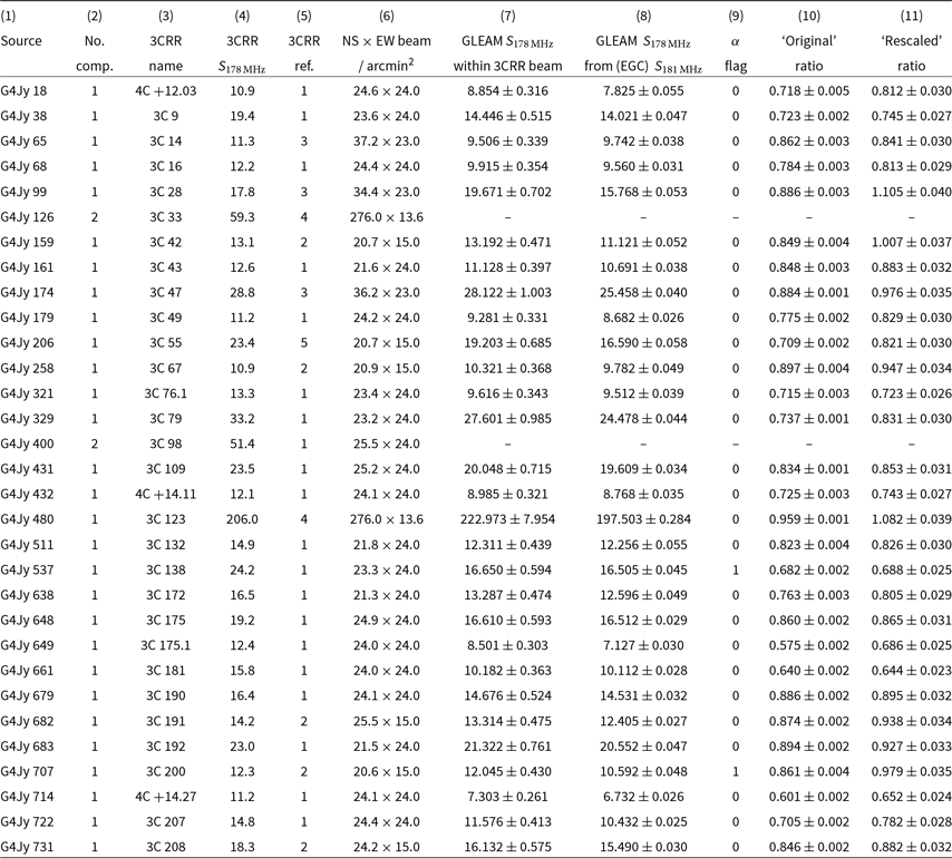
Table 8. Continued – The 67 G4Jy sources that are also in the 3CRR sample. Note that beam dimensions cannot be provided for 3CRR sources that have an interpolated/extrapolated  $S_{\textrm{178\,MHz}}$
(3CRR ref. = 6). Hence, the remaining columns for these sources are also left unfilled. Due to space considerations, we note here that columns 4, 7, and 8 are in units of Jy.
$S_{\textrm{178\,MHz}}$
(3CRR ref. = 6). Hence, the remaining columns for these sources are also left unfilled. Due to space considerations, we note here that columns 4, 7, and 8 are in units of Jy.
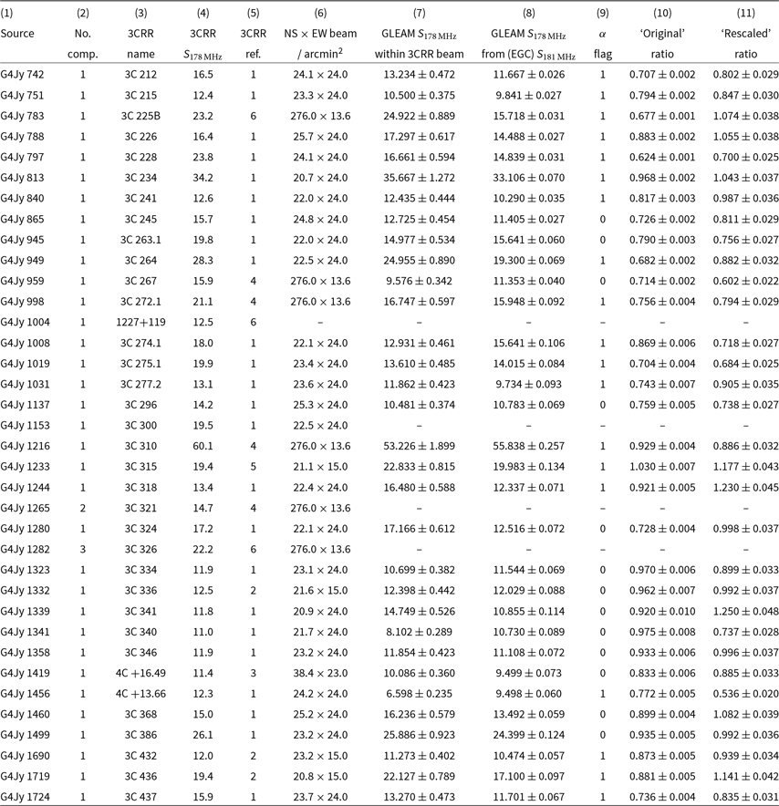
7.3. Flux density comparison with 3CRR
The G4Jy Sample will enable further investigation of relativistic jets and their interaction with the environment, as already explored using the well-studied 3CRR sample. Given the prominence of the latter, we conduct a flux density analysis for 67 G4Jy sources that overlap with 3CRR (following on from Section 7.1.5). These are listed in Table 8.
First, the closest GLEAM flux density measurement we have to  $S_{\textrm{178\,MHz}}$
is that for the 181-MHz sub-band. We extrapolate this to 178 MHz by assuming a power-law description of the radio emission and using the spectral index (G4Jy_alpha) fitted to the G4Jy total flux densities (Sections 6.5 and 6.6). Where the associated reduced-
$S_{\textrm{178\,MHz}}$
is that for the 181-MHz sub-band. We extrapolate this to 178 MHz by assuming a power-law description of the radio emission and using the spectral index (G4Jy_alpha) fitted to the G4Jy total flux densities (Sections 6.5 and 6.6). Where the associated reduced- $\chi^2$
value is
$\chi^2$
value is  $>1.93$
, we instead use the spectral index provided in the 3CRR catalogue (obtained through VizieR) for this extrapolation. The ratio of GLEAM
$>1.93$
, we instead use the spectral index provided in the 3CRR catalogue (obtained through VizieR) for this extrapolation. The ratio of GLEAM  $S_{\textrm{178\,MHz}}$
to 3CRR
$S_{\textrm{178\,MHz}}$
to 3CRR  $S_{\textrm{178\,MHz}}$
is presented in Table 8 as the ‘original’ ratio. Looking at the distribution of this ratio (Figure 10), we see that the GLEAM flux density appears to be systematically lower than that measured for 3CRR. Note that the 3CRR catalogue does not provide errors for
$S_{\textrm{178\,MHz}}$
is presented in Table 8 as the ‘original’ ratio. Looking at the distribution of this ratio (Figure 10), we see that the GLEAM flux density appears to be systematically lower than that measured for 3CRR. Note that the 3CRR catalogue does not provide errors for  $S_{\textrm{178\,MHz}}$
(nor for the spectral index), but it uses the RBC scale of Roger et al. (Reference Roger, Bridle and Costain1973),a which is known to differ by
$S_{\textrm{178\,MHz}}$
(nor for the spectral index), but it uses the RBC scale of Roger et al. (Reference Roger, Bridle and Costain1973),a which is known to differ by  $\sim$
9% from the KPW scale (Kellermann et al. Reference Kellermann, Pauliny-Toth and Williams1969) at 178 MHz (Laing & Peacock Reference Laing and Peacock1980; Laing et al. Reference Laing, Riley and Longair1983). Meanwhile, the EGC has an uncertainty in the flux density scale of
$\sim$
9% from the KPW scale (Kellermann et al. Reference Kellermann, Pauliny-Toth and Williams1969) at 178 MHz (Laing & Peacock Reference Laing and Peacock1980; Laing et al. Reference Laing, Riley and Longair1983). Meanwhile, the EGC has an uncertainty in the flux density scale of  $8.0\pm0.5$
% for sources at
$8.0\pm0.5$
% for sources at  $-72.0^{\circ}<$
Dec.
$-72.0^{\circ}<$
Dec. $<18.5^{\circ}$
and
$<18.5^{\circ}$
and  $11\pm2$
% for sources at Dec.
$11\pm2$
% for sources at Dec. $>18.5^{\circ}$
(Hurley-Walker et al. Reference Hurley-Walker2017). However, a combination of the two flux density scale errors (where we consider the extreme fractional errors of 0.09 and 0.13)
$>18.5^{\circ}$
(Hurley-Walker et al. Reference Hurley-Walker2017). However, a combination of the two flux density scale errors (where we consider the extreme fractional errors of 0.09 and 0.13)
is not enough to explain the discrepancy for the 23 G4Jy–3CRR sources with ratio $<0.78$
.
$<0.78$
.
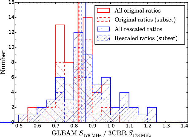
Figure 10. The ratio of  $S_{\textrm{178\,MHz}}$
measured using GLEAM data, to
$S_{\textrm{178\,MHz}}$
measured using GLEAM data, to  $S_{\textrm{178\,MHz}}$
using the 3CRR catalogue (Laing et al. Reference Laing, Riley and Longair1983). These are for 60 of the 67 3CRR sources that overlap with the G4Jy Sample, where ‘original ratios’ refers to the 3CRR
$S_{\textrm{178\,MHz}}$
using the 3CRR catalogue (Laing et al. Reference Laing, Riley and Longair1983). These are for 60 of the 67 3CRR sources that overlap with the G4Jy Sample, where ‘original ratios’ refers to the 3CRR  $S_{\textrm{178\,MHz}}$
being the value provided in the 3CRR catalogue. The median original ratio is 0.82 and is indicated by a thick, vertical, red, solid line. ‘Rescaled ratios’ are those where the 3CRR
$S_{\textrm{178\,MHz}}$
being the value provided in the 3CRR catalogue. The median original ratio is 0.82 and is indicated by a thick, vertical, red, solid line. ‘Rescaled ratios’ are those where the 3CRR  $S_{\textrm{178\,MHz}}$
value has had its corresponding beam size (Table 8) taken into account, leading to rescaling of this flux density (see Section 7.3 for details). The median rescaled ratio is 0.87 and is indicated by a thick, vertical, blue, solid line. For both sets of ratios, the GLEAM
$S_{\textrm{178\,MHz}}$
value has had its corresponding beam size (Table 8) taken into account, leading to rescaling of this flux density (see Section 7.3 for details). The median rescaled ratio is 0.87 and is indicated by a thick, vertical, blue, solid line. For both sets of ratios, the GLEAM  $S_{\textrm{178\,MHz}}$
value is extrapolated from the
$S_{\textrm{178\,MHz}}$
value is extrapolated from the  $S_{\textrm{181\,MHz}}$
measurement in the EGC (Hurley-Walker et al. Reference Hurley-Walker2017). Meanwhile, ‘subset’ (see legend) refers to the G4Jy sources for which we are able to use the G4Jy spectral index for extrapolating flux densities from one frequency to another (as indicated by
$S_{\textrm{181\,MHz}}$
measurement in the EGC (Hurley-Walker et al. Reference Hurley-Walker2017). Meanwhile, ‘subset’ (see legend) refers to the G4Jy sources for which we are able to use the G4Jy spectral index for extrapolating flux densities from one frequency to another (as indicated by  $\alpha$
flag = ‘0’ in Table 8). The thick, vertical, dashed lines indicate the median values for this subset, with respect to the original ratios (median = 0.83; red) and rescaled ratios (median = 0.84; blue).
$\alpha$
flag = ‘0’ in Table 8). The thick, vertical, dashed lines indicate the median values for this subset, with respect to the original ratios (median = 0.83; red) and rescaled ratios (median = 0.84; blue).
Next, we note that the 178-MHz flux densities in the 3CRR catalogue are a compilation from numerous surveys: 4CT, 4C, and 3CR (see references in caption of Table 8). Each of these surveys was conducted using a beam ranging from 19 to 235 times larger (by area) than that of the MWA, prompting us to investigate whether confusion/unrelated emission could account for the 3CRR flux densities being systematically higher than those from GLEAM.
As Aegean may underestimate the flux density for extended sources, we only consider for the analysis G4Jy–3CRR sources that are characterised by a single GLEAM component. For each of these sources, we apply an ellipse, of the relevant beam dimensions (column 6 of Table 8), to the 181-MHz sub-band image from GLEAM.Footnote q We then use the solid angle of the MWA beam to calculate the integrated flux density over this ellipse (which involves summing over all pixel values within the ellipse and normalising with respect to the beam). In addition, we wish to characterise how well this method is able to reproduce the 181-MHz, integrated flux density measurement that is provided in the EGC. For this, we apply an ellipse of dimensions fitted by Aegean (i.e. the semi-major and semi-major axes, a_181 and b_181, respectively), along with the fitted position angle (pa_181), and again calculate the integrated flux density over the ellipse. The mean ratio of this ellipse-derived  $S_{\textrm{181\,MHz}}$
to the original EGC
$S_{\textrm{181\,MHz}}$
to the original EGC  $S_{\textrm{181\,MHz}}$
then allows us to ‘correct’ other flux densities determined in a similar way. Similarly, we use the standard deviation in the ratio to estimate the error in the integrated flux density calculated over an ellipse. The result is a corrected GLEAM
$S_{\textrm{181\,MHz}}$
then allows us to ‘correct’ other flux densities determined in a similar way. Similarly, we use the standard deviation in the ratio to estimate the error in the integrated flux density calculated over an ellipse. The result is a corrected GLEAM  $S_{\textrm{181\,MHz}}$
measured within the ‘3CRR’ beam, which we then extrapolate to 178 MHz (again using either G4Jy_alpha or the 3CRR spectral index, as previously). The extrapolated value is what appears in column 7 of Table 8.
$S_{\textrm{181\,MHz}}$
measured within the ‘3CRR’ beam, which we then extrapolate to 178 MHz (again using either G4Jy_alpha or the 3CRR spectral index, as previously). The extrapolated value is what appears in column 7 of Table 8.
How much extra emission is detected through the large beam associated with 3CRR, compared to the fitted GLEAM measurement, is apparent from comparing columns 7 and 8 of Table 8. Dividing the latter by the former then gives a ‘corrective factor’, which we use to rescale the 3CRR  $S_{\textrm{178\,MHz}}$
. The ‘re-scaled’ ratio (column 11) is the ratio of the GLEAM
$S_{\textrm{178\,MHz}}$
. The ‘re-scaled’ ratio (column 11) is the ratio of the GLEAM  $S_{\textrm{178\,MHz}}$
(column 8) to this rescaled 3CRR
$S_{\textrm{178\,MHz}}$
(column 8) to this rescaled 3CRR  $S_{\textrm{178\,MHz}}$
. As shown in Figure 10, these rescaled ratios (mean
$S_{\textrm{178\,MHz}}$
. As shown in Figure 10, these rescaled ratios (mean  $= 0.87 \pm 0.16$
) are closer to 1.0 than the original ratios (mean
$= 0.87 \pm 0.16$
) are closer to 1.0 than the original ratios (mean  $= 0.81 \pm 0.11$
), but more-widely distributed, and now as large as 1.25. Therefore, whilst unrelated emission may still play a part, we cannot conclude that it is the main reason for the offset between GLEAM and 3CRR flux densities. Furthermore, a two-sample Kolmogorov–Smirnov test gives D = 0.27 (where 0.30 is the D statistic to exceed) and p-value = 0.02, indicating that the two distributions are not significantly distinct.
$= 0.81 \pm 0.11$
), but more-widely distributed, and now as large as 1.25. Therefore, whilst unrelated emission may still play a part, we cannot conclude that it is the main reason for the offset between GLEAM and 3CRR flux densities. Furthermore, a two-sample Kolmogorov–Smirnov test gives D = 0.27 (where 0.30 is the D statistic to exceed) and p-value = 0.02, indicating that the two distributions are not significantly distinct.
We now return to an explanation that has already been touched upon in this sub-section: that the flux density calibration of GLEAM components is worse at the highest declinations. Whilst this is true for the GLEAM catalogue as a whole, we see no trend in the GLEAM  $S_{\textrm{178\,MHz}}$
/3CRR
$S_{\textrm{178\,MHz}}$
/3CRR  $S_{\textrm{178\,MHz}}$
ratio with declination, as shown in Figure 11a. We also see no trend in the ratio with the integrated flux density of the source (Figure 11b), but cannot use this to rule out non-linearity in the flux scale calibration. This is because the overlap of the G4Jy Sample with 3CRR restricts our investigation to
$S_{\textrm{178\,MHz}}$
ratio with declination, as shown in Figure 11a. We also see no trend in the ratio with the integrated flux density of the source (Figure 11b), but cannot use this to rule out non-linearity in the flux scale calibration. This is because the overlap of the G4Jy Sample with 3CRR restricts our investigation to  $S_{\textrm{178\,MHz}}\,{\gtrsim}\,10.9\,\text{Jy}$
sources, whereas one of the criteria used to select sources for setting the GLEAM flux density scale (
$S_{\textrm{178\,MHz}}\,{\gtrsim}\,10.9\,\text{Jy}$
sources, whereas one of the criteria used to select sources for setting the GLEAM flux density scale ( $S_{\textrm{74\,MHz}}>2\,\text{Jy}$
; Hurley-Walker et al. Reference Hurley-Walker2017) corresponds to
$S_{\textrm{74\,MHz}}>2\,\text{Jy}$
; Hurley-Walker et al. Reference Hurley-Walker2017) corresponds to  $S_{\textrm{178\,MHz}}\,{\gtrsim}\,1\,\text{Jy}$
(assuming
$S_{\textrm{178\,MHz}}\,{\gtrsim}\,1\,\text{Jy}$
(assuming  $S_{\nu} \propto \nu^{-0.7}$
). It is possible that the flux density scale starts to show non-linearity (Scott & Shakeshaft Reference Scott and Shakeshaft1971; Laing & Peacock Reference Laing and Peacock1980) as the 10.9-Jy threshold is approached, but further investigation is beyond the scope of this work. In addition, Eddington bias may be affecting 3CRR sources detected at lower signal to noise (as weakly suggested by Figure 11b), leading to the 3CRR
$S_{\nu} \propto \nu^{-0.7}$
). It is possible that the flux density scale starts to show non-linearity (Scott & Shakeshaft Reference Scott and Shakeshaft1971; Laing & Peacock Reference Laing and Peacock1980) as the 10.9-Jy threshold is approached, but further investigation is beyond the scope of this work. In addition, Eddington bias may be affecting 3CRR sources detected at lower signal to noise (as weakly suggested by Figure 11b), leading to the 3CRR  $S_{\textrm{178\,MHz}}$
being overestimated. However, this is difficult to explore further due to the absence of
$S_{\textrm{178\,MHz}}$
being overestimated. However, this is difficult to explore further due to the absence of  $S_{\textrm{178\,MHz}}$
uncertainties in the 3CRR catalogue.
$S_{\textrm{178\,MHz}}$
uncertainties in the 3CRR catalogue.
Next, we plot the total, integrated flux densities across the GLEAM band (72–231 MHz) alongside previous multi-frequency measurements for the 3CRR sample. For this, we include the G4Jy–3CRR sources that have multiple GLEAM components associated with them. The resulting SEDs (spanning 10 MHz to 15 GHz) are available as online supplementary material (Appendix F) and confirm that the G4Jy flux densities are consistently lower for this subset of very bright sources at high declination. Although we are unable to conclusively state the reason(s) for this offset, we point out that the G4Jy catalogue inherits from the EGC the internal-calibration consistency of  $\leq$
3%, as determined over 245,457 GLEAM components (Hurley-Walker et al. Reference Hurley-Walker2017). Furthermore, recent P-band (230–470 MHz) VLA observations of
$\leq$
3%, as determined over 245,457 GLEAM components (Hurley-Walker et al. Reference Hurley-Walker2017). Furthermore, recent P-band (230–470 MHz) VLA observations of  $\sim$
40 unresolved sources suggest that the GLEAM flux density scale is
$\sim$
40 unresolved sources suggest that the GLEAM flux density scale is  $\sim$
3% too low (Callingham et al., in preparation). This is based on a comparison of the
$\sim$
3% too low (Callingham et al., in preparation). This is based on a comparison of the  $S_{\textrm{230\,MHz}}$
measurement from GLEAM and the expected flux density at 230 MHz, following spectral fitting of the GLEAM and P-band data. The latter are tied to the flux-density scale of Perley & Butler (Reference Perley and Butler2017), over 50 MHz to 50 GHz.
$S_{\textrm{230\,MHz}}$
measurement from GLEAM and the expected flux density at 230 MHz, following spectral fitting of the GLEAM and P-band data. The latter are tied to the flux-density scale of Perley & Butler (Reference Perley and Butler2017), over 50 MHz to 50 GHz.
Table 10. Characteristics of the G4Jy Sample (Section 7.4), in terms of the number of GLEAM components associated with an individual source, and the morphology of the NVSS/SUMSS emission (Section 5.2).
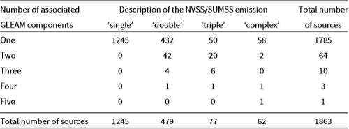
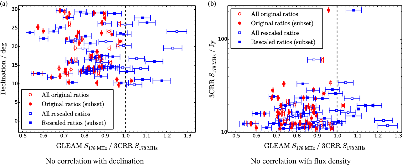
Figure 11. The GLEAM  $S_{\textrm{178\,MHz}}$
/3CRR
$S_{\textrm{178\,MHz}}$
/3CRR  $S_{\textrm{178\,MHz}}$
ratio plotted against (a) declination and (b) 3CRR
$S_{\textrm{178\,MHz}}$
ratio plotted against (a) declination and (b) 3CRR  $S_{\textrm{178\,MHz}}$
. These are for 60 of the 67 3CRR sources that overlap with the G4Jy Sample, where ‘original ratios’ refers to the 3CRR
$S_{\textrm{178\,MHz}}$
. These are for 60 of the 67 3CRR sources that overlap with the G4Jy Sample, where ‘original ratios’ refers to the 3CRR  $S_{\textrm{178\,MHz}}$
value being that provided in the 3CRR catalogue. ‘Rescaled ratios’ are those where the 3CRR
$S_{\textrm{178\,MHz}}$
value being that provided in the 3CRR catalogue. ‘Rescaled ratios’ are those where the 3CRR  $S_{\textrm{178\,MHz}}$
value has had its corresponding beam size (Table 8) taken into account, leading to rescaling of this flux density (see Section 7.3 for details). As in Figure 10, ‘subset’ (see legends) refers to the G4Jy sources for which we are able to use the G4Jy spectral index for extrapolating flux densities from one frequency to another (as indicated by
$S_{\textrm{178\,MHz}}$
value has had its corresponding beam size (Table 8) taken into account, leading to rescaling of this flux density (see Section 7.3 for details). As in Figure 10, ‘subset’ (see legends) refers to the G4Jy sources for which we are able to use the G4Jy spectral index for extrapolating flux densities from one frequency to another (as indicated by  $\alpha$
flag = ‘0’ in Table 8). For both panels, the vertical, black, dashed line is where the ratio is equal to 1.0, to guide the eye.
$\alpha$
flag = ‘0’ in Table 8). For both panels, the vertical, black, dashed line is where the ratio is equal to 1.0, to guide the eye.
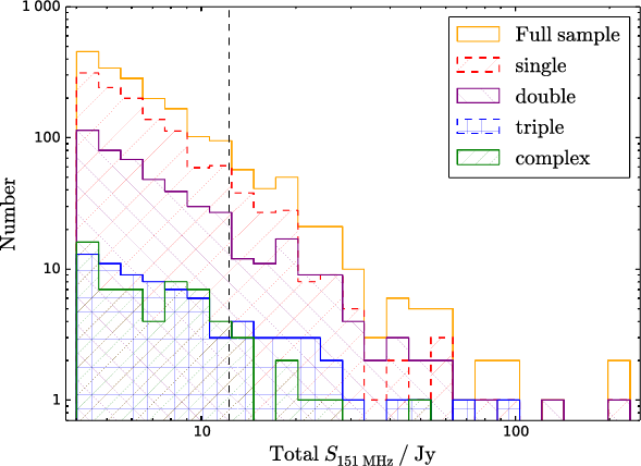
Figure 12. The distribution in  $S_{\textrm{151\,MHz}}$
for the full sample, and when split by morphology (‘single’, ‘double’, ‘triple’, and ‘complex’) in NVSS/SUMSS/TGSS (Section 5.2 and 7.4). The vertical line is where
$S_{\textrm{151\,MHz}}$
for the full sample, and when split by morphology (‘single’, ‘double’, ‘triple’, and ‘complex’) in NVSS/SUMSS/TGSS (Section 5.2 and 7.4). The vertical line is where  $S_{\textrm{151\,MHz}} = 12.2\,\text{Jy}$
, which corresponds to
$S_{\textrm{151\,MHz}} = 12.2\,\text{Jy}$
, which corresponds to  $S_{\textrm{178\,MHz}} = 10.9\,\text{Jy}$
(assuming a power-law radio spectrum with spectral index,
$S_{\textrm{178\,MHz}} = 10.9\,\text{Jy}$
(assuming a power-law radio spectrum with spectral index,  $\alpha = -0.7$
). Therefore, the G4Jy sources to the right of the vertical line are akin to those in the 3CRR sample (Laing et al. Reference Laing, Riley and Longair1983).
$\alpha = -0.7$
). Therefore, the G4Jy sources to the right of the vertical line are akin to those in the 3CRR sample (Laing et al. Reference Laing, Riley and Longair1983).
7.4. Summary of the results from visual inspection and checks for completeness
As a result of our visual inspection and further checks, the original list of 1879 GLEAM components becomes a list of 1 960 components. In conjunction, this is reduced to a list of 1 863 GLEAM sources, and it is this source list that we refer to as the G4Jy Sample. 67% of the G4Jy sources are ‘singles’, 26% are ‘doubles’, 4% are ‘triples’, and 3% have ‘complex’ morphology (Table 10). In Figure 12, we show the distributions in  $S_{\textrm{151\,MHz}}$
for these subsets, in addition to that for the full sample. We note that there are 233 G4Jy sources brighter than 12.2 Jy at 151 MHz, which corresponds to the flux density limit for the 3CRR sample (173 sources). Of these sources, the fraction that are a ‘double’ or a ‘triple’ is 41%, whilst for the 1630 G4Jy sources below this threshold, the fraction falls to 28%. Without redshifts to consider the radio luminosities, we hypothesise that the brighter sources are likely to be closer and more extended, and therefore resolved in NVSS/SUMSS/TGSS (which are the surveys we use to determine the morphology). Meanwhile, it is important to note that 21% (383) of the G4Jy sources are affected by confusion (Section 5.2), and so the GLEAM flux densities will need to be updated in the future.
$S_{\textrm{151\,MHz}}$
for these subsets, in addition to that for the full sample. We note that there are 233 G4Jy sources brighter than 12.2 Jy at 151 MHz, which corresponds to the flux density limit for the 3CRR sample (173 sources). Of these sources, the fraction that are a ‘double’ or a ‘triple’ is 41%, whilst for the 1630 G4Jy sources below this threshold, the fraction falls to 28%. Without redshifts to consider the radio luminosities, we hypothesise that the brighter sources are likely to be closer and more extended, and therefore resolved in NVSS/SUMSS/TGSS (which are the surveys we use to determine the morphology). Meanwhile, it is important to note that 21% (383) of the G4Jy sources are affected by confusion (Section 5.2), and so the GLEAM flux densities will need to be updated in the future.
Following our best efforts, the G4Jy Sample of  $S_{\textrm{151\,MHz}}>4\,\text{Jy}$
radio sources is effectively complete over the footprint of the EGC (Hurley-Walker et al. Reference Hurley-Walker2017) minus the region defined as
$S_{\textrm{151\,MHz}}>4\,\text{Jy}$
radio sources is effectively complete over the footprint of the EGC (Hurley-Walker et al. Reference Hurley-Walker2017) minus the region defined as  $-18.3^{\circ} < b < -10.0^{\circ}$
,
$-18.3^{\circ} < b < -10.0^{\circ}$
,  $65.4^{\circ} < l < 81.1^{\circ}$
, Dec.
$65.4^{\circ} < l < 81.1^{\circ}$
, Dec. $<30.0^{\circ}$
(Section 7.1.5). This covers
$<30.0^{\circ}$
(Section 7.1.5). This covers  $24\,731 \text{deg}^2$
(i.e. 60% of the entire sky), all of which is accessible to the SKA and its precursor telescopes. The sky density of the G4Jy Sample is therefore one source per
$24\,731 \text{deg}^2$
(i.e. 60% of the entire sky), all of which is accessible to the SKA and its precursor telescopes. The sky density of the G4Jy Sample is therefore one source per  $\sim13\,\text{deg}^2$
. Within this total sky area, we know that at least one
$\sim13\,\text{deg}^2$
. Within this total sky area, we know that at least one  $>4\,\text{Jy}$
source is absent (Orion A; see Section 3.1) and acknowledge that we may still be missing a few extended radio sources. Hence, we estimate that the G4Jy Sample is 99.50–99.95% complete. In addition, the brightest G4Jy source (G4Jy 1402; 3C 353) is at
$>4\,\text{Jy}$
source is absent (Orion A; see Section 3.1) and acknowledge that we may still be missing a few extended radio sources. Hence, we estimate that the G4Jy Sample is 99.50–99.95% complete. In addition, the brightest G4Jy source (G4Jy 1402; 3C 353) is at  $S_{\textrm{151\,MHz}}=232\,\text{Jy}$
, with our sample being biased against sources that are brighter than this (namely, ‘A-team’ sources, which are masked for the EGC; see Table 1).
$S_{\textrm{151\,MHz}}=232\,\text{Jy}$
, with our sample being biased against sources that are brighter than this (namely, ‘A-team’ sources, which are masked for the EGC; see Table 1).
Finally, in light of a  $\sim$
3% offset (Callingham et al., in preparation; Section 7.3) between the flux-density scale of GLEAM and that of Perley & Butler (Reference Perley and Butler2017), we consider the effect that this would have on the completeness of the G4Jy Sample. We find that there are 88 GLEAM components in the EGC at
$\sim$
3% offset (Callingham et al., in preparation; Section 7.3) between the flux-density scale of GLEAM and that of Perley & Butler (Reference Perley and Butler2017), we consider the effect that this would have on the completeness of the G4Jy Sample. We find that there are 88 GLEAM components in the EGC at  $3.89 < S_{\textrm{151\,MHz}}\textrm{/Jy}< 4.00$
that would then need to be considered for inclusion. One of these is GLEAM J151635+001603, which is already in the sample as being associated with GLEAM J151643+001410 (together composing G4Jy 1238). Similarly, some of the remaining 87 components may be associated with each other, but equally, some components
$3.89 < S_{\textrm{151\,MHz}}\textrm{/Jy}< 4.00$
that would then need to be considered for inclusion. One of these is GLEAM J151635+001603, which is already in the sample as being associated with GLEAM J151643+001410 (together composing G4Jy 1238). Similarly, some of the remaining 87 components may be associated with each other, but equally, some components  $<$
3.89 Jy may sum together to
$<$
3.89 Jy may sum together to  $>\,3.89\,\text{Jy}$
(cf. Sections 7.1 and 7.2, regarding the 4-Jy threshold). Therefore, for simplicity (and remembering that Orion A is absent from the considered footprint), we estimate the completeness to be
$>\,3.89\,\text{Jy}$
(cf. Sections 7.1 and 7.2, regarding the 4-Jy threshold). Therefore, for simplicity (and remembering that Orion A is absent from the considered footprint), we estimate the completeness to be  $1863 / (1863 + 87 +1) = 95.5$
% on the flux-density scale of Perley & Butler (Reference Perley and Butler2017).
$1863 / (1863 + 87 +1) = 95.5$
% on the flux-density scale of Perley & Butler (Reference Perley and Butler2017).
8. Initial and future analyses
Having produced a thorough compilation of the brightest radio sources in the southern sky, we use the G4Jy catalogue to perform some initial analysis, which we describe in this section. This will be followed by full-sample multi-wavelength analysis in Paper III of the G4Jy series and investigation into broadband radio spectra (covering 72 MHz–20 GHz) to be presented in Paper IV. In addition, we will compare our association of components observed at  $\sim1\,\text{GHz}$
(White & Line in preparation) with the results obtained using the Positional Update and Matching Algorithm (PUMA; Line et al. Reference Line, Webster, Pindor, Mitchell and Trott2017). We envisage that this can be extended to using the G4Jy Sample as a training set for machine-learning algorithms, and so leveraging the effort that we have put into host galaxy identification (which is summarised in Section 5.5 and detailed in Paper II).
$\sim1\,\text{GHz}$
(White & Line in preparation) with the results obtained using the Positional Update and Matching Algorithm (PUMA; Line et al. Reference Line, Webster, Pindor, Mitchell and Trott2017). We envisage that this can be extended to using the G4Jy Sample as a training set for machine-learning algorithms, and so leveraging the effort that we have put into host galaxy identification (which is summarised in Section 5.5 and detailed in Paper II).
8.1. Angular size information
An overview of linear, physical sizes for G4Jy sources will be provided in Paper III, as calculating these sizes is reliant on redshifts being compiled for the sample. These may reveal that additional sources are GRGs, further to those listed in Table 3 of Paper II.
In the meantime, we can obtain sample-wide information by considering the distribution in the angular sizes of the 1 863 sources, since we know how the angular size scale (kpc/arcsec) varies with redshift. This distribution is presented in Figure 13, where the median angular size of 43.8 arcsec is marked by a vertical, dashed line. (Note that for this analysis, we fix all angular sizes to their upper limits. This is applicable for 855 sources, with the largest upper limit being 129.8 arcsec.) As shown in the left-hand panels of Figure 13, at least half of the G4Jy Sample is smaller than 370 kpc, regardless of redshift. Furthermore, if a source is  $\,{\gtrsim}\,$
500 arcsec in angular size, its physical size must be at least 100 kpc, even at the very low redshift of 0.01 (Figure 13b). However, we remind the reader that the angular sizes are derived using NVSS or SUMSS (Section 6.3.1), and so are limited by the 45 arcsec resolution of these surveys. If we consider only the 657 sources that are multi-component in NVSS or SUMSS, we find that the median angular size is 74.5 arcsec.
$\,{\gtrsim}\,$
500 arcsec in angular size, its physical size must be at least 100 kpc, even at the very low redshift of 0.01 (Figure 13b). However, we remind the reader that the angular sizes are derived using NVSS or SUMSS (Section 6.3.1), and so are limited by the 45 arcsec resolution of these surveys. If we consider only the 657 sources that are multi-component in NVSS or SUMSS, we find that the median angular size is 74.5 arcsec.
Table 11. 22 G4Jy sources previously identified by Chhetri et al. (Reference Chhetri, Morgan, Ekers, Macquart, Sadler, Giroletti, Callingham and Tingay2018) as showing moderate ( $0.4\,{\leq}\,$
NSI
$0.4\,{\leq}\,$
NSI $\,{<}\,0.9$
) or strong (NSI
$\,{<}\,0.9$
) or strong (NSI $\,{\geq}\,0.9$
) interplanetary scintillation (Section 8.1). NSI = normalised scintillation index.
$\,{\geq}\,0.9$
) interplanetary scintillation (Section 8.1). NSI = normalised scintillation index.
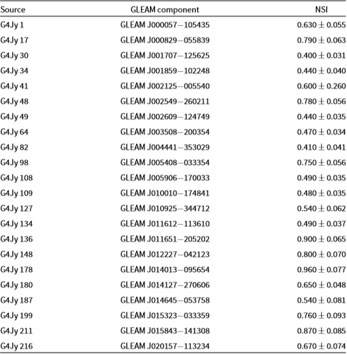
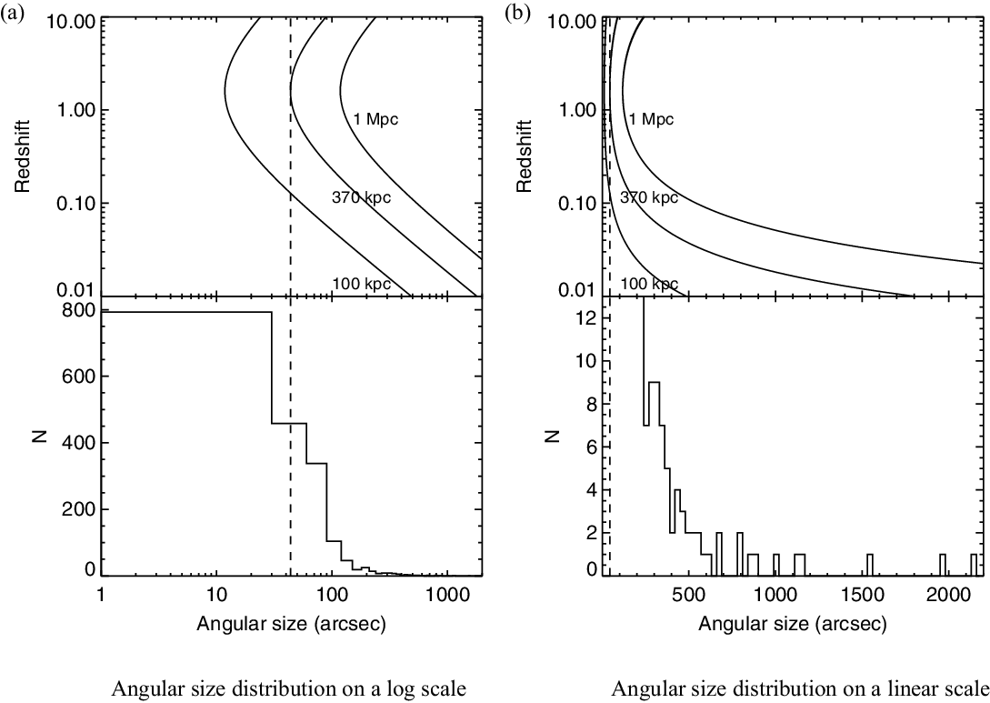
Figure 13. The solid lines in the upper panels of this figure show how the observed angular size varies with redshift for a source of fixed physical size (100 kpc, 370 kpc, 1 Mpc). These functions are calculated in accordance with the cosmology described at the end of Section 1. The lower panels show the angular size distribution for sources in the G4Jy Sample, with the median angular size marked by a dashed, vertical line (Section 8.1).
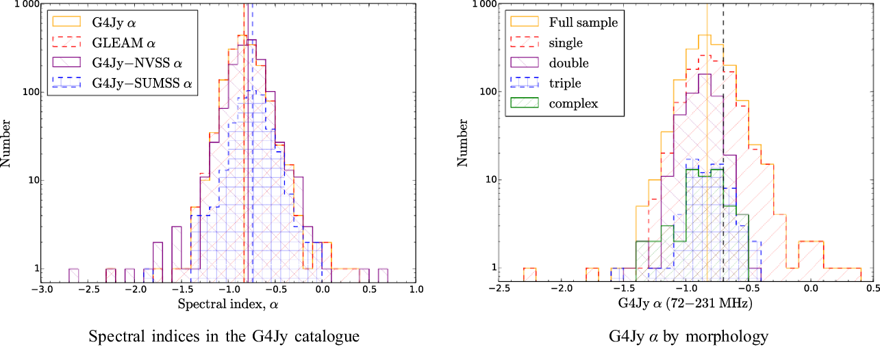
Figure 14. (a) The distributions for the four sets of spectral index provided in the G4Jy catalogue: G4Jy  $\alpha$
, GLEAM
$\alpha$
, GLEAM  $\alpha$
, G4Jy–NVSS
$\alpha$
, G4Jy–NVSS  $\alpha$
, and G4Jy–SUMSS
$\alpha$
, and G4Jy–SUMSS  $\alpha$
(see Section 6.6). The median values for each spectral index are indicated by vertical lines (using the same colour and linestyle as for the corresponding histogram; see legend). (b) The distribution in G4Jy
$\alpha$
(see Section 6.6). The median values for each spectral index are indicated by vertical lines (using the same colour and linestyle as for the corresponding histogram; see legend). (b) The distribution in G4Jy  $\alpha$
for the full sample, and for sources with ‘single’, ‘double’, ‘triple’, and ‘complex’ morphology in NVSS/SUMSS/TGSS (Sections 5.2 and 8.2). The black, dashed, vertical line is where
$\alpha$
for the full sample, and for sources with ‘single’, ‘double’, ‘triple’, and ‘complex’ morphology in NVSS/SUMSS/TGSS (Sections 5.2 and 8.2). The black, dashed, vertical line is where  $\alpha = -0.7$
, which is the canonical spectral index that we use for extrapolation of flux densities (assuming
$\alpha = -0.7$
, which is the canonical spectral index that we use for extrapolation of flux densities (assuming  $S_{\nu} \propto \nu^{\alpha}$
). For comparison, we also plot the median G4Jy
$S_{\nu} \propto \nu^{\alpha}$
). For comparison, we also plot the median G4Jy  $\alpha$
value for the full sample (orange, solid, vertical line).
$\alpha$
value for the full sample (orange, solid, vertical line).
Next, particularly with unresolved G4Jy sources in mind, we explore the compactness of the radio emission by considering whether the source exhibits interplanetary scintillation (Little & Hewish Reference Little and Hewish1966; Morgan et al. Reference Morgan2018). This is where radio sources appear to ‘twinkle’ due to the turbulence of the intervening solar wind, allowing sub-arcsecond scales to be probed. Chhetri et al. (Reference Chhetri, Morgan, Ekers, Macquart, Sadler, Giroletti, Callingham and Tingay2018) demonstrated the power of this method over  $30\times30\,\text{deg}^2$
(i.e. the field of view for a single MWA pointing) by characterising the scintillation properties of 2 550 sources. In total, 131 of these sources are in the G4Jy Sample, with two being described as ‘strong’ scintillators (normalised scintillation index, NSI
$30\times30\,\text{deg}^2$
(i.e. the field of view for a single MWA pointing) by characterising the scintillation properties of 2 550 sources. In total, 131 of these sources are in the G4Jy Sample, with two being described as ‘strong’ scintillators (normalised scintillation index, NSI  $\geq0.9$
). This means that a single sub-arcsecond component is dominating the flux density at 162 MHz (their observing frequency). Another 20 sources are ‘moderate’ scintillators (
$\geq0.9$
). This means that a single sub-arcsecond component is dominating the flux density at 162 MHz (their observing frequency). Another 20 sources are ‘moderate’ scintillators ( $0.4\leq$
NSI
$0.4\leq$
NSI  $<0.9$
), which may include sources with multiple sub-arcsecond components, and sources where there is a single sub-arcsecond component but it is surrounded by more-extended low-frequency emission. The 22 moderate/strong scintillators cross-matched with the G4Jy Sample are listed in Table 11. However, another 43 of the 131 cross-matched sources may also have compact emission on sub-arcsecond scales, but for them Chhetri et al. (Reference Chhetri, Morgan, Ekers, Macquart, Sadler, Giroletti, Callingham and Tingay2018) could only provide upper limits in NSI, due to the scintillation not reaching the detection threshold.
$<0.9$
), which may include sources with multiple sub-arcsecond components, and sources where there is a single sub-arcsecond component but it is surrounded by more-extended low-frequency emission. The 22 moderate/strong scintillators cross-matched with the G4Jy Sample are listed in Table 11. However, another 43 of the 131 cross-matched sources may also have compact emission on sub-arcsecond scales, but for them Chhetri et al. (Reference Chhetri, Morgan, Ekers, Macquart, Sadler, Giroletti, Callingham and Tingay2018) could only provide upper limits in NSI, due to the scintillation not reaching the detection threshold.
8.2. Spectral information
In Figure 14a, we present the distributions for each of the four spectral indices that we provide in the G4Jy catalogue (see Section 6.6). Although these refer to the ‘full sample’, we remind the reader that a different number of G4Jy sources (or GLEAM components, as the case may be) is used for each distribution, as indicated in Table 3. In the following analysis,  $\alpha^{\textrm{231\,MHz}}_{\textrm{72\,MHz}} = \text{G4Jy}\ \alpha$
,
$\alpha^{\textrm{231\,MHz}}_{\textrm{72\,MHz}} = \text{G4Jy}\ \alpha$
,  $\alpha^{\textrm{1400\,MHz}}_{\textrm{151\,MHz}} = \text{G4Jy--NVSS} \alpha$
, and
$\alpha^{\textrm{1400\,MHz}}_{\textrm{151\,MHz}} = \text{G4Jy--NVSS} \alpha$
, and  $\alpha^{\textrm{843\,MHz}}_{\textrm{151\,MHz}} = \text{G4Jy--SUMSS} \alpha$
(with each assuming radio emission of the spectral form,
$\alpha^{\textrm{843\,MHz}}_{\textrm{151\,MHz}} = \text{G4Jy--SUMSS} \alpha$
(with each assuming radio emission of the spectral form,  $S_{\nu} \propto \nu^{\alpha}$
).
$S_{\nu} \propto \nu^{\alpha}$
).
Table 12. 67 G4Jy sources previously identified by Callingham et al. (Reference Callingham2017) as having a spectral peak at a frequency ( $\nu_{\textrm{peak}}$
) between 72 and 1400 MHz (Section 8.2). G4Jy 136 and G4Jy 178 are the strong scintillators mentioned in Section 8.1.
$\nu_{\textrm{peak}}$
) between 72 and 1400 MHz (Section 8.2). G4Jy 136 and G4Jy 178 are the strong scintillators mentioned in Section 8.1.
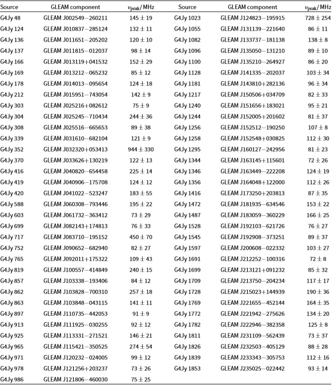
Note that for the majority of the sample (i.e. 1603/1863 = 86% of the sources), a power-law spectrum is an accurate description of the total radio emission between 72 and 231 MHz. If this were not the case, the reduced- $\chi^2$
value corresponding to
$\chi^2$
value corresponding to  $\alpha^{\textrm{231\,MHz}}_{\textrm{72\,MHz}}$
(the ‘G4Jy_alpha’ column in the G4Jy catalogue) would be
$\alpha^{\textrm{231\,MHz}}_{\textrm{72\,MHz}}$
(the ‘G4Jy_alpha’ column in the G4Jy catalogue) would be  $>1.93,$
and we would mask the spectral index for the catalogue. Therefore, for the remaining 14% of sources, the radio emission shows evidence of spectral curvature within the GLEAM band. Further evidence of curvature is apparent from the median value for the low-frequency spectral index (
$>1.93,$
and we would mask the spectral index for the catalogue. Therefore, for the remaining 14% of sources, the radio emission shows evidence of spectral curvature within the GLEAM band. Further evidence of curvature is apparent from the median value for the low-frequency spectral index ( $\alpha^{\textrm{231\,MHz}}_{\textrm{72\,MHz}}$
) being steeper than the median value for the spectral index calculated between 151 MHz and 843 MHz/1400 MHz (
$\alpha^{\textrm{231\,MHz}}_{\textrm{72\,MHz}}$
) being steeper than the median value for the spectral index calculated between 151 MHz and 843 MHz/1400 MHz ( $\alpha^{\textrm{843\,MHz}}_{\textrm{151\,MHz}}$
/
$\alpha^{\textrm{843\,MHz}}_{\textrm{151\,MHz}}$
/ $\alpha^{\textrm{1400\,MHz}}_{\textrm{151\,MHz}}$
, respectively)—see Table 3 and the vertical lines in Figure 14a. The reasons for this will be discussed further in Papers III and IV, following additional analysis (White et al., in preparation).
$\alpha^{\textrm{1400\,MHz}}_{\textrm{151\,MHz}}$
, respectively)—see Table 3 and the vertical lines in Figure 14a. The reasons for this will be discussed further in Papers III and IV, following additional analysis (White et al., in preparation).
Conversely, a source with a flatter spectrum within the GLEAM band than towards higher frequencies (i.e.  $\alpha^{\textrm{231\,MHz}}_{\textrm{72\,MHz}} > \alpha^{\textrm{843\,MHz}}_{\textrm{151\,MHz}}$
or
$\alpha^{\textrm{231\,MHz}}_{\textrm{72\,MHz}} > \alpha^{\textrm{843\,MHz}}_{\textrm{151\,MHz}}$
or  $\alpha^{\textrm{1400\,MHz}}_{\textrm{151\,MHz}}$
) is likely to be turning over due to free-free absorption or synchrotron self-absorption (Lacki Reference Lacki2013). Such sources have previously been identified in the EGC by Callingham et al. (Reference Callingham2017), and in cross-matching the G4Jy Sample with their catalogues, we find an overlap of one GHz-peaked spectrum (GPS) source (G4Jy 1533; GLEAM J192451
$\alpha^{\textrm{1400\,MHz}}_{\textrm{151\,MHz}}$
) is likely to be turning over due to free-free absorption or synchrotron self-absorption (Lacki Reference Lacki2013). Such sources have previously been identified in the EGC by Callingham et al. (Reference Callingham2017), and in cross-matching the G4Jy Sample with their catalogues, we find an overlap of one GHz-peaked spectrum (GPS) source (G4Jy 1533; GLEAM J192451 $-$
291426), 67 sources with a spectral peak between 72 and 1400 MHz (listed in Table 12), and 19 sources with a spectral peak below 72 MHz (listed in Table 13). Each of these sources is ‘single’ in morphology, with the exception of G4Jy 1233 (GLEAM J151340+260718), which we label as ‘complex’. This is due to its X-shaped morphology, which is shown in Figure 4d of Paper II. Furthermore, G4Jy 352, G4Jy 420, G4Jy 819, G4Jy 965, G4Jy 1597, G4Jy 1772, and G4Jy 1801 are 7 of 15 sources found to have low-frequency variability by Bell et al. (Reference Bell2019), who use a preliminary version of the G4Jy Sample for their study.
$-$
291426), 67 sources with a spectral peak between 72 and 1400 MHz (listed in Table 12), and 19 sources with a spectral peak below 72 MHz (listed in Table 13). Each of these sources is ‘single’ in morphology, with the exception of G4Jy 1233 (GLEAM J151340+260718), which we label as ‘complex’. This is due to its X-shaped morphology, which is shown in Figure 4d of Paper II. Furthermore, G4Jy 352, G4Jy 420, G4Jy 819, G4Jy 965, G4Jy 1597, G4Jy 1772, and G4Jy 1801 are 7 of 15 sources found to have low-frequency variability by Bell et al. (Reference Bell2019), who use a preliminary version of the G4Jy Sample for their study.
Returning to the distribution in  $\alpha^{\textrm{231\,MHz}}_{\textrm{72\,MHz}}$
for the full sample, we also present this spectral index for each of the categories in morphology (Figure 14b). The ‘doubles’ and ‘triples’ have (mostly) steep spectral indices that span a range of
$\alpha^{\textrm{231\,MHz}}_{\textrm{72\,MHz}}$
for the full sample, we also present this spectral index for each of the categories in morphology (Figure 14b). The ‘doubles’ and ‘triples’ have (mostly) steep spectral indices that span a range of  $-1.6$
to
$-1.6$
to  $-0.4$
, which is as expected if the lobes are dominating the radio emission. Meanwhile, for ‘single’ sources, the range in
$-0.4$
, which is as expected if the lobes are dominating the radio emission. Meanwhile, for ‘single’ sources, the range in  $\alpha^{\textrm{231\,MHz}}_{\textrm{72\,MHz}}$
is considerably wider from
$\alpha^{\textrm{231\,MHz}}_{\textrm{72\,MHz}}$
is considerably wider from  $-2.3$
to
$-2.3$
to  $0.4$
. This subset encompasses ultra-steep sources at high redshift and flat-spectrum sources (where the core is believed to be dominating the radio emission).Footnote r However, this is complicated by the size of the MWA beam, which leads to G4Jy/GLEAM flux densities being affected by confusion. As a result, the fitted spectral index of the G4Jy source differs from its true value.
$0.4$
. This subset encompasses ultra-steep sources at high redshift and flat-spectrum sources (where the core is believed to be dominating the radio emission).Footnote r However, this is complicated by the size of the MWA beam, which leads to G4Jy/GLEAM flux densities being affected by confusion. As a result, the fitted spectral index of the G4Jy source differs from its true value.
9. Summary
Due to radio sources exhibiting a great variety of morphologies, identifying the correct host galaxy (if appropriate) is a difficult task. We have invested considerable effort into this for the brightest radio sources in the GLEAM EGC, including repeated visual inspection and thorough time-intensive consultation of the literature (see Paper II for details on individual sources). Here we summarise the work done in defining the GLEAM 4-Jy (G4Jy) Sample (i.e. sources with  $S_{\textrm{151\,MHz}}>4\,\text{Jy}$
) and preparing the G4Jy catalogue:
$S_{\textrm{151\,MHz}}>4\,\text{Jy}$
) and preparing the G4Jy catalogue:
i. We confirm that ‘A-team’ sources, the Magellanic Clouds, and the Orion Nebula all have
$S_{\textrm{151\,MHz}}>4\,\text{Jy}$
but are not in the G4Jy Sample, following their absence from the parent catalogue, EGC. However, we provide an estimate of the integrated flux density for these sources for reference.
ii. Since the MWA provides
${\sim}2$
arcmin resolution, we use the better spatial resolution of TGSS, NVSS, and SUMSS to interpret the morphology of the brightest radio sources in the southern sky. This allows us to determine what radio emission is associated together and which G4Jy sources are affected by confusion. We also use NVSS and SUMSS to calculate the summed flux density and angular size at
${\sim}\,1\,\text{GHz}$
.iii. In addition, we use the NVSS/SUMSS components to calculate brightness-weighted centroid positions, which aid our identification of the host galaxy in the mid-infrared. The latter is done through visual inspection, and all images and overlays are made available online (see https://github.com/svw26/G4Jy for details).
iv. When inspecting the overlays, we remind the user to be aware of artefacts in NVSS, SUMSS, and TGSS. We characterise the TGSS artefacts in terms of position angle and angular separation, with respect to the G4Jy source, as this has not been done before.
v. The G4Jy catalogue contains 10 GLEAM components (corresponding to 6 G4Jy sources) that have been refitted using Aegean, which is the source-finding software used to create the EGC. As such, the GLEAM flux densities for these components do not appear in the parent catalogue.
vi. Also within our value-added catalogue are AllWISE host galaxy positions (and magnitudes) for 1606 of the 1863 sources in the G4Jy Sample. In the case of a cluster relic and a nebula, identifying a ‘host’ is inappropriate, so these fields are left blank. The remaining sources either have a host galaxy that is not in the AllWISE catalogue or there is uncertainty as to the correct identification. The latter are being followed up using MeerKAT Open Time (PI: White), to confirm the position of the radio core.
vii. 78 G4Jy sources are resolved into multiple GLEAM components by the MWA Phase-I beam. Therefore, we provide integrated flux densities summed over these components, per source, and indicate their association via our source-naming scheme. Whilst the GLEAM-band spectral index is inherited from the EGC per GLEAM component (for all but the refitted components), we use the summed, integrated flux densities to recalculate this spectral index per G4Jy source. In addition, we use the total
$S_{\textrm{151\,MHz}}$
to determine the spectral index between 151 MHz and
$\sim1\,\text{GHz}$
(assuming a power-law description,
$S_{\nu} \propto \nu^{\alpha}$
).viii. In order to improve the completeness of the G4Jy Sample, we perform cross-checks against existing radio source samples and use internal matching of the EGC to identify extended sources that would otherwise have been missed. Following this, we estimate that the sample is 99.50–99.95% complete to
$S_{\textrm{151\,MHz}}=4\,\text{Jy}$
on the GLEAM flux density scale, which corresponds to a completeness of 95.5% on the flux density scale of Perley & Butler (Reference Perley and Butler2017).ix. Note that the above estimates of sample completeness are relevant over the footprint of the EGC minus the region defined by
$-18.3^{\circ} < b < -10.0^{\circ}$
,
$65.4^{\circ} < l < 81.1^{\circ}$
, Dec.
$<30.0^{\circ}$
. The reason for this subtraction is that GLEAM flux densities are not well characterised over this area of the sky, due to the influence of Cygnus A.x. Of the 173 radio galaxies belonging to the well-studied 3CRR sample, 67 of these overlap with the G4Jy Sample. We compare the GLEAM flux density at 178 MHz to that provided in the 3CRR catalogue and find that the GLEAM value is systematically lower. However, we note that this may be due to several factors: the larger ‘3CRR’ beams detecting unrelated emission, errors (and possible non-linearity) in the flux-density scales of the two catalogues, and that the GLEAM calibration error is worse at these high declinations (
$>10^{\circ}$
).xi. Preliminary analysis of the full sample shows that the median angular size (at 843/1400 MHz) is 43.8 arcsec, and that the radio spectrum is more often steeper at low frequencies (72–231 MHz) than between 151 and 843/1400 MHz. For the ‘doubles’ and ‘triples’ that make up 30% of the sample, the 72–231 MHz spectral index spans a range of
$-1.6$
to
$-0.4$
, as expected for lobe-dominated radio sources. However, 21% of the G4Jy Sample has low-frequency flux densities that may be affected by confusion, and so these measurements and the derived spectral indices should be treated with caution.


Table 13. 19 G4Jy sources previously identified by Callingham et al. (Reference Callingham2017) as having a spectral peak below 72 MHz (Section 8.2).

The result of many iterations, between the G4Jy catalogue and accompanying overlays, is a firm base upon which this legacy dataset can be reliably cross-matched with information at other wavelengths. Such a large, complete, unbiased radio source sample is required for investigating, for example, the production of powerful jets and their interaction with the environment. Furthermore, by exploiting the excellent spectral coverage provided by the MWA, we can tightly constrain the spectral behaviour of the G4Jy sources and determine the prevalence of ‘restarted’ AGN activity.
10. Dedication
Papers I and II are dedicated to the memory of Richard Hunstead, who was very helpful with the assessment of the sources presented in this work, and provided hitherto unpublished radio images.
Acknowledgements
The authors thank the anonymous referee for their time in reviewing our manuscript. SVW would like to thank Chris Jordan, for his help with installing and running the cross-matching software (MCVCM), as well as Dave Pallot and the ICRAR Data Intensive Astronomy team, for their help with fixing and updating the G4Jy Sample Server. In addition, SVW thanks Ron Ekers, Robert Laing, Elaine Sadler, Tom Mauch, and Huib Intema for useful discussions. The authors acknowledge the International Centre for Radio Astronomy Research (ICRAR), which is a joint venture between Curtin University and The University of Western Australia, funded by the Western Australian State government. The authors acknowledge the Pawsey Supercomputing Centre which is supported by the Western Australian and Australian Governments. The financial assistance of the South African Radio Astronomy Observatory (SARAO) towards this research is hereby acknowledged ().
This scientific work makes use of the Murchison Radio-astronomy Observatory, operated by CSIRO. The authors acknowledge the Wajarri Yamatji people as the traditional owners of the Observatory site. Support for the operation of the MWA is provided by the Australian Government (NCRIS), under a contract to Curtin University administered by Astronomy Australia Limited.
GMRT is run by the National Centre for Radio Astrophysics of the Tata Institute of Fundamental Research (TIFR). The Australia Telescope Compact Array (ATCA) is part of the Australia Telescope National Facility which is funded by the Australian Government for operation as a National Facility managed by CSIRO.
This publication made use of data products from the Wide-field Infrared Survey Explorer, which is a joint project of the University of California, Los Angeles, and the Jet Propulsion Laboratory/California Institute of Technology, funded by the National Aeronautics and Space Administration (NASA).
This research has made use of the NASA/IPAC Extragalactic Database (NED), which is operated by the Jet Propulsion Laboratory, California Institute of Technology, under contract with the National Aeronautics and Space Administration. The authors also acknowledge the use of NASA’s SkyView facility (http://skyview.gsfc.nasa.gov) located at NASA Goddard Space Flight Center. This research has made use of the SIMBAD astronomical database (Wenger et al. Reference Wenger2000), operated at CDS, Strasbourg, France.
This research has made use of the VizieR catalogue access tool, CDS, Strasbourg, France (DOI: 10.26093/cds/vizier). The original description of the VizieR service was published in A&AS 143, 23 (Ochsenbein, Bauer, & Marcout Reference Ochsenbein, Bauer and Marcout2000).
This research made use of Montage. It is funded by the National Science Foundation under Grant Number ACI-1440620 and was previously funded by the National Aeronautics and Space Administration’s Earth Science Technology Office, Computation Technologies Project, under Cooperative Agreement Number NCC5-626 between NASA and the California Institute of Technology.
Finally, the following open-source software was used for data visualisation and processing: topcat (Taylor Reference Taylor, Systems, Shopbell, Britton and Ebert2005), SAOImage DS9 (Smithsonian Astrophysical Observatory 2000; Joye & Mandel Reference Joye, Mandel, Systems, Payne, Jedrzejewski and Hook2003), NumPy (Oliphant Reference Oliphant2006), Astropy (Astropy Collaboration et al. 2013), APLpy (Robitaille & Bressert, Reference Robitaille and Bressert2012), Matplotlib (Hunter Reference Hunter2007), and SciPy (Jones et al. Reference Jones2001).
Supplementary Material
To view supplementary material for this article, please visit https://doi.org/10.1017/pasa.2020.9.
A. The Orion Nebula
The GLEAM images of Orion A resolve the nebula into a rough trapezoid about  $30'\times25'$
in size and a 5-diameter circular source to the north-east. We use the poly_flux scriptFootnote s to determine integrated flux density measurements covering the entire nebula. This software calculates a background level from a region surrounding the object of interest, excluding any selected regions, which in this case we set to obvious areas of unrelated emission. The flux density measurements at 88, 118, 154, and 200 MHz are, respectively,
$30'\times25'$
in size and a 5-diameter circular source to the north-east. We use the poly_flux scriptFootnote s to determine integrated flux density measurements covering the entire nebula. This software calculates a background level from a region surrounding the object of interest, excluding any selected regions, which in this case we set to obvious areas of unrelated emission. The flux density measurements at 88, 118, 154, and 200 MHz are, respectively,  $22.8\pm1.8$
,
$22.8\pm1.8$
,  $46.3\pm3.7$
,
$46.3\pm3.7$
,  $65.7\pm5.3$
, and
$65.7\pm5.3$
, and  $81.8\pm6.5\,\text{Jy}$
. The measurement errors are dominated by the 8% flux density accuracy of GLEAM at this declination.
$81.8\pm6.5\,\text{Jy}$
. The measurement errors are dominated by the 8% flux density accuracy of GLEAM at this declination.
Terzian & Parrish (Reference Terzian and Parrish1970) used the Arecibo Observatory to measure the flux density of the Orion Nebula at 73.8, 111.5, and 196.5 MHz, measuring flux densities of  $32\pm15$
,
$32\pm15$
,  $62\pm7$
, and
$62\pm7$
, and  $108\pm11\,\text{Jy}$
, respectively. The resolution of Arecibo at these frequencies is
$108\pm11\,\text{Jy}$
, respectively. The resolution of Arecibo at these frequencies is  $85'\times120'$
,
$85'\times120'$
,  $54'\times77'$
, and
$54'\times77'$
, and  $33'\times43 {.\mkern-4mu^\prime}5$
, respectively. The larger values measured by this instrument are due to its low-resolution beam confusing surrounding radio sources with emission from the nebula.Footnote t We correct for this confusion by measuring the flux density contained within ellipses of the beam size, centred on the Orion Nebula, and comparing it to GLEAM measurements, deriving correction factors at 154 MHz. These correction factors are 54%, 64%, and 76%, respectively, leading to corrected values of
$33'\times43 {.\mkern-4mu^\prime}5$
, respectively. The larger values measured by this instrument are due to its low-resolution beam confusing surrounding radio sources with emission from the nebula.Footnote t We correct for this confusion by measuring the flux density contained within ellipses of the beam size, centred on the Orion Nebula, and comparing it to GLEAM measurements, deriving correction factors at 154 MHz. These correction factors are 54%, 64%, and 76%, respectively, leading to corrected values of  $17\pm8$
,
$17\pm8$
,  $40\pm4$
, and
$40\pm4$
, and  $82\pm8\,\text{Jy}$
, respectively.
$82\pm8\,\text{Jy}$
, respectively.
We fit a curved spectrum to the data, of the form  $S_{\nu}\propto\nu^\alpha \exp{q(\ln{\nu})^2}$
. Using solely the GLEAM measurements, we obtain
$S_{\nu}\propto\nu^\alpha \exp{q(\ln{\nu})^2}$
. Using solely the GLEAM measurements, we obtain  $S_\textrm{151\,MHz}=67.3\pm0.1\,\text{Jy}$
, while including the corrected data from Terzian & Parrish (Reference Terzian and Parrish1970) yields
$S_\textrm{151\,MHz}=67.3\pm0.1\,\text{Jy}$
, while including the corrected data from Terzian & Parrish (Reference Terzian and Parrish1970) yields 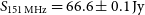 $S_\textrm{151\,MHz}=66.6\pm0.1\,\text{Jy}$
. This is remarkably close given the simplicity of the correction method. The shape of the spectrum is identical, with
$S_\textrm{151\,MHz}=66.6\pm0.1\,\text{Jy}$
. This is remarkably close given the simplicity of the correction method. The shape of the spectrum is identical, with  $\alpha=1.1\pm0.2$
and
$\alpha=1.1\pm0.2$
and  $q=-1.5\pm0.5$
.
$q=-1.5\pm0.5$
.
B. GLEAM components removed from the G4Jy Sample
Five GLEAM components with  $S_{\textrm{151\,MHz}}>4\,\text{Jy}$
were removed from the G4Jy Sample (Section 5.2), following the initial selection (Section 3). This is because multiple unrelated sources were identified through visual inspection of their overlays (Figure B1), suggesting that confused GLEAM emission was the reason for these components appearing above the selection threshold. This is supported by flux density measurements at higher spatial resolution from TGSS, which indicate that no single source is likely to have
$S_{\textrm{151\,MHz}}>4\,\text{Jy}$
were removed from the G4Jy Sample (Section 5.2), following the initial selection (Section 3). This is because multiple unrelated sources were identified through visual inspection of their overlays (Figure B1), suggesting that confused GLEAM emission was the reason for these components appearing above the selection threshold. This is supported by flux density measurements at higher spatial resolution from TGSS, which indicate that no single source is likely to have  $S_{\textrm{151\,MHz}}>4\,\text{Jy}$
. Details are provided here for reference, including the relevant TGSS flux densities (
$S_{\textrm{151\,MHz}}>4\,\text{Jy}$
. Details are provided here for reference, including the relevant TGSS flux densities ( $S_{\textrm{150\,MHz}}$
).
$S_{\textrm{150\,MHz}}$
).
Figure B1. Overlays for five GLEAM components that were removed from the G4Jy sample, following visual inspection and investigation of the relative flux densities for the confused sources (Section 5.2). The contours, symbols, and beams are the same as for Figure 1, with AllWISE positions (green plus signs) within 3 arcmin of the centroid position (purple hexagon) also plotted. (a) GLEAM J093918+015948. (b) GLEAM J101051−020137. (c) GLEAM J201707−310305. (d) GLEAM J202336−191144. (e) GLEAM J222751−303344.
GLEAM J093918+015948:  $S_{\textrm{151\,MHz}} = 4.55 \pm 0.03 \,\text{Jy}$
. Two unrelated sources with
$S_{\textrm{151\,MHz}} = 4.55 \pm 0.03 \,\text{Jy}$
. Two unrelated sources with  $S_{\textrm{150\,MHz}} = 4.40$
, 1.08 Jy. We note that a correction needs to be applied in order for the TGSS catalogue to have the same flux scale as GLEAM (Hurley-Walker Reference Hurley-Walker2017), but for this work, we are only interested in the relative flux densities of sources that are confused by the MWA beam. Here, the brighter source accounts for 80% of the total TGSS emission. This corresponds to 3.66 Jy at 151 MHz in GLEAM.
$S_{\textrm{150\,MHz}} = 4.40$
, 1.08 Jy. We note that a correction needs to be applied in order for the TGSS catalogue to have the same flux scale as GLEAM (Hurley-Walker Reference Hurley-Walker2017), but for this work, we are only interested in the relative flux densities of sources that are confused by the MWA beam. Here, the brighter source accounts for 80% of the total TGSS emission. This corresponds to 3.66 Jy at 151 MHz in GLEAM.
GLEAM J101051  $-$
020137:
$-$
020137:  $S_{\textrm{151\,MHz}} = 4.81 \pm 0.03 \,\text{Jy}$
. This GLEAM component is dominated by two unrelated point sources (
$S_{\textrm{151\,MHz}} = 4.81 \pm 0.03 \,\text{Jy}$
. This GLEAM component is dominated by two unrelated point sources ( $S_{\textrm{150\,MHz}} = 3.31$
, 2.18Jy), with two fainter sources (
$S_{\textrm{150\,MHz}} = 3.31$
, 2.18Jy), with two fainter sources ( $S_{\textrm{150\,MHz}} = 0.06$
, 0.04 Jy) nearby. None of the sources are above the 4-Jy threshold at 151 MHz.
$S_{\textrm{150\,MHz}} = 0.06$
, 0.04 Jy) nearby. None of the sources are above the 4-Jy threshold at 151 MHz.
GLEAM J201707  $-$
310305:
$-$
310305:  $S_{\textrm{151\,MHz}} = 4.60 \pm 0.06 \,\text{Jy}$
. We agree with Jones & McAdam (Reference Jones and McAdam1992), regarding 2014
$S_{\textrm{151\,MHz}} = 4.60 \pm 0.06 \,\text{Jy}$
. We agree with Jones & McAdam (Reference Jones and McAdam1992), regarding 2014 $-$
312, that the bulk of the radio emission is from a ‘double’ (
$-$
312, that the bulk of the radio emission is from a ‘double’ ( $S_{\textrm{150\,MHz}} = 1.74 + 1.27 = 3.01\,\text{Jy}$
) and two point sources (
$S_{\textrm{150\,MHz}} = 1.74 + 1.27 = 3.01\,\text{Jy}$
) and two point sources ( $S_{\textrm{150\,MHz}} = 1.14$
, 0.93 Jy) to the east of this. The confused source (
$S_{\textrm{150\,MHz}} = 1.14$
, 0.93 Jy) to the east of this. The confused source ( $S_{\textrm{150\,MHz}} = 0.07\,\text{Jy}$
) towards the north is also considered, but none of these sources have
$S_{\textrm{150\,MHz}} = 0.07\,\text{Jy}$
) towards the north is also considered, but none of these sources have  $S_{\textrm{151\,MHz}} > 4\,\text{Jy}$
. Based on the presence of a bright mid-infrared source between the two point sources, we also consider the possibility that they are associated and form another ‘double’. However, its summed flux density (
$S_{\textrm{151\,MHz}} > 4\,\text{Jy}$
. Based on the presence of a bright mid-infrared source between the two point sources, we also consider the possibility that they are associated and form another ‘double’. However, its summed flux density ( $S_{\textrm{150\,MHz}} = 1.14 + 0.93 = 2.07\,\text{Jy}$
) would still be too low to warrant retaining this GLEAM component for the G4Jy Sample.
$S_{\textrm{150\,MHz}} = 1.14 + 0.93 = 2.07\,\text{Jy}$
) would still be too low to warrant retaining this GLEAM component for the G4Jy Sample.
GLEAM J202336  $-$
191144:
$-$
191144:  $S_{\textrm{151\,MHz}} = 4.54 \pm 0.05 \,\text{Jy}$
. Two unrelated sources with
$S_{\textrm{151\,MHz}} = 4.54 \pm 0.05 \,\text{Jy}$
. Two unrelated sources with  $S_{\textrm{150\,MHz}} = 3.47$
, 1.08 Jy. Neither source is above the 4-Jy threshold at 151 MHz.
$S_{\textrm{150\,MHz}} = 3.47$
, 1.08 Jy. Neither source is above the 4-Jy threshold at 151 MHz.
GLEAM J222751  $-$
303344:
$-$
303344:  $S_{\textrm{151\,MHz}} = 4.40 \pm 0.02 \,\text{Jy}$
. The MWA beam has blended emission from a ‘compact’ source (
$S_{\textrm{151\,MHz}} = 4.40 \pm 0.02 \,\text{Jy}$
. The MWA beam has blended emission from a ‘compact’ source ( $S_{\textrm{150\,MHz}} = 1.23\,\text{Jy}$
) and a head-tail galaxy to the north-west (
$S_{\textrm{150\,MHz}} = 1.23\,\text{Jy}$
) and a head-tail galaxy to the north-west (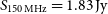 $S_{\textrm{150\,MHz}} = 1.83\,\text{Jy}$
). This interpretation is based upon a VLA observation of 2225
$S_{\textrm{150\,MHz}} = 1.83\,\text{Jy}$
). This interpretation is based upon a VLA observation of 2225 $-$
308 by Ekers et al. (Reference Ekers1989). However, we draw attention to the unusual extension of the TGSS contours (
$-$
308 by Ekers et al. (Reference Ekers1989). However, we draw attention to the unusual extension of the TGSS contours ( $S_{\textrm{150\,MHz}} = 0.53$
, 0.17 Jy) compared to the NVSS contours. The TGSS contours suggest that the compact radio source may in fact be a ‘triple’, with old, lobe emission evident only at low radio frequencies. Even if the three southern-most TGSS components are associated, the integrated flux density is still insufficient for the southern source to cross the 4-Jy threshold.
$S_{\textrm{150\,MHz}} = 0.53$
, 0.17 Jy) compared to the NVSS contours. The TGSS contours suggest that the compact radio source may in fact be a ‘triple’, with old, lobe emission evident only at low radio frequencies. Even if the three southern-most TGSS components are associated, the integrated flux density is still insufficient for the southern source to cross the 4-Jy threshold.
C. Multi-component G4Jy sources
Table C1 lists all of the G4Jy sources that have multiple GLEAM components. We also present overlays for 30 of these sources (Figures C1–C5) that are not shown elsewhere in Paper I (Figures 1, 3–9, D1, D3) nor in Paper II (Figures 3–4, 6, 8, 12, 16–17, 19, 21, 23).
D. Details of Aegean refitting
This appendix provides details as to GLEAM components—identified through visual inspection—that require refitting (Section 5.3). The source-finding software, Aegean (Hancock et al. Reference Hancock, Murphy, Gaensler, Hopkins and Curran2012; Reference Hancock, Trott and Hurley-Walker2018), is used in different modes for this procedure, as described in the following subsections. The resulting refitted components follow the same naming system as for the EGC (Hurley-Walker et al. Reference Hurley-Walker2017) and are used for the G4Jy catalogue (Section 6; Appendix E) and overlays.
Table C1. The 78 G4Jy sources that have multiple GLEAM components. (Their radio/mid-infrared overlays are shown in numerous figures throughout the paper, with 30 of them presented in Appendix C.) For 54 sources, just one component needed to have  $S_{\textrm{151\,MHz}}>4\,\text{Jy}$
in order to be selected for the sample (Section 3). Other components were then identified via visual inspection (Section 5) and become part of the G4Jy Sample by association. Note that the GLEAM components associated with G4Jy 1080, 1677, 1678, 1704, and 1705 do not appear in the GLEAM EGC (Hurley-Walker et al. Reference Hurley-Walker2017), as these are the result of refitting with Aegean (Appendix D). In addition, for 24 multi-component sources, none of the GLEAM components are in the original selection, but further work (Section 7) leads to their inclusion in the G4Jy Sample. In this table, we remove the ‘GLEAM’ prefix of the GLEAM-component name.
$S_{\textrm{151\,MHz}}>4\,\text{Jy}$
in order to be selected for the sample (Section 3). Other components were then identified via visual inspection (Section 5) and become part of the G4Jy Sample by association. Note that the GLEAM components associated with G4Jy 1080, 1677, 1678, 1704, and 1705 do not appear in the GLEAM EGC (Hurley-Walker et al. Reference Hurley-Walker2017), as these are the result of refitting with Aegean (Appendix D). In addition, for 24 multi-component sources, none of the GLEAM components are in the original selection, but further work (Section 7) leads to their inclusion in the G4Jy Sample. In this table, we remove the ‘GLEAM’ prefix of the GLEAM-component name.
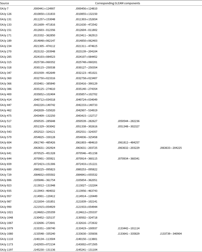
Table C1. Continued - G4Jy sources with multiple GLEAM components.
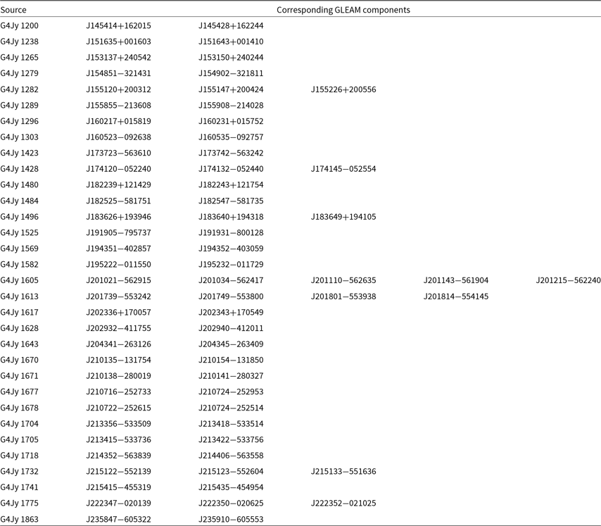
D.1. Unconstrained refitting
The value of inspecting large images is most apparent for radio sources with very extended emission. Based on the original 20 arcmin overlays, it was thought that GLEAM J133549 $-$
335247 and GLEAM J133637
$-$
335247 and GLEAM J133637 $-$
335724 were associated, but ‘zooming out’ revealed that these components accounted for only one of the lobes belonging to an extended radio galaxy (Figure 1). The reason that this was not appreciated earlier is that the second lobe is within the masked region (a
$-$
335724 were associated, but ‘zooming out’ revealed that these components accounted for only one of the lobes belonging to an extended radio galaxy (Figure 1). The reason that this was not appreciated earlier is that the second lobe is within the masked region (a  $\text{circle of radius} = 9^{\circ}$
) used to exclude Centaurus A from the GLEAM catalogue (Hurley-Walker et al. Reference Hurley-Walker2017). Consequently, we refit this ‘bisected’ source using Aegean. Without the constraints imposed by the previously applied mask, we find that four GLEAM components describe the low-frequency emission of G4Jy 1080: GLEAM J133548
$\text{circle of radius} = 9^{\circ}$
) used to exclude Centaurus A from the GLEAM catalogue (Hurley-Walker et al. Reference Hurley-Walker2017). Consequently, we refit this ‘bisected’ source using Aegean. Without the constraints imposed by the previously applied mask, we find that four GLEAM components describe the low-frequency emission of G4Jy 1080: GLEAM J133548 $-$
335240, GLEAM J133630
$-$
335240, GLEAM J133630 $-$
335656, GLEAM J133641
$-$
335656, GLEAM J133641 $-$
335829, and GLEAM J133739
$-$
335829, and GLEAM J133739 $-$
340904. We add these components to the GLEAM-component list and remove GLEAM J133549
$-$
340904. We add these components to the GLEAM-component list and remove GLEAM J133549 $-$
335247 and GLEAM J133637
$-$
335247 and GLEAM J133637 $-$
335724.
$-$
335724.
Also known as IC 4296, this refitted source is the brightest cluster galaxy (BCG) of Abell 3565, which is part of the Hydra–Centaurus Supercluster. Being at  $z=0.012$
(Mahony et al. Reference Mahony2011), the galaxy’s lobe-to-lobe extent of 33 arcmin corresponds to a physical scale of 487 kpc (Wright Reference Wright2006). In addition, we note that the backflow of plasma in the southern lobe is only indicated by the MWA contours (Figure 1), thanks to the instrument’s sensitivity to diffuse emission.
$z=0.012$
(Mahony et al. Reference Mahony2011), the galaxy’s lobe-to-lobe extent of 33 arcmin corresponds to a physical scale of 487 kpc (Wright Reference Wright2006). In addition, we note that the backflow of plasma in the southern lobe is only indicated by the MWA contours (Figure 1), thanks to the instrument’s sensitivity to diffuse emission.
D.2. Peeled sources
Due to the regular arrangement of dipoles in its component tiles, the primary beam of the MWA has regularly spaced sidelobes, which can have high sensitivity, typically  $\approx$
10% at low frequencies and high elevations, and up to 100% at high frequencies and low elevations. For some pointings of GLEAM, bright sources appeared in these sidelobes and needed to be removed from the visibilities before self-calibration could be performed. Hurley-Walker et al. (Reference Hurley-Walker2017) used a ‘peeling’ technique, in which the visibilities are phase-rotated to the source, a calibration solution is formed, and the solution applied to the model of the source, then subtracted from the visibilities, which are then phase-rotated back to the original pointing direction for self-calibration and imaging. However, to perfectly predict which observations need peeling and which do not, the model of the primary beam and the flux densities of the sources must be perfectly known, and this was not the case during the GLEAM data processing.
$\approx$
10% at low frequencies and high elevations, and up to 100% at high frequencies and low elevations. For some pointings of GLEAM, bright sources appeared in these sidelobes and needed to be removed from the visibilities before self-calibration could be performed. Hurley-Walker et al. (Reference Hurley-Walker2017) used a ‘peeling’ technique, in which the visibilities are phase-rotated to the source, a calibration solution is formed, and the solution applied to the model of the source, then subtracted from the visibilities, which are then phase-rotated back to the original pointing direction for self-calibration and imaging. However, to perfectly predict which observations need peeling and which do not, the model of the primary beam and the flux densities of the sources must be perfectly known, and this was not the case during the GLEAM data processing.

Figure C1. Overlays for G4Jy sources that have multiple GLEAM components (Table C1, Appendix C). The datasets, contours, symbols, and beams are the same as those used for Figure 1, but where blue contours, crosses, and ellipses correspond to NVSS or SUMSS. In addition, positions from AllWISE are indicated by green plus signs, with cross-identified host galaxies highlighted in white. (a) G4Jy 7. (b) G4Jy 126. (c) G4Jy 360. (d) G4Jy 366. (e) G4Jy 386. (f) G4Jy 400.
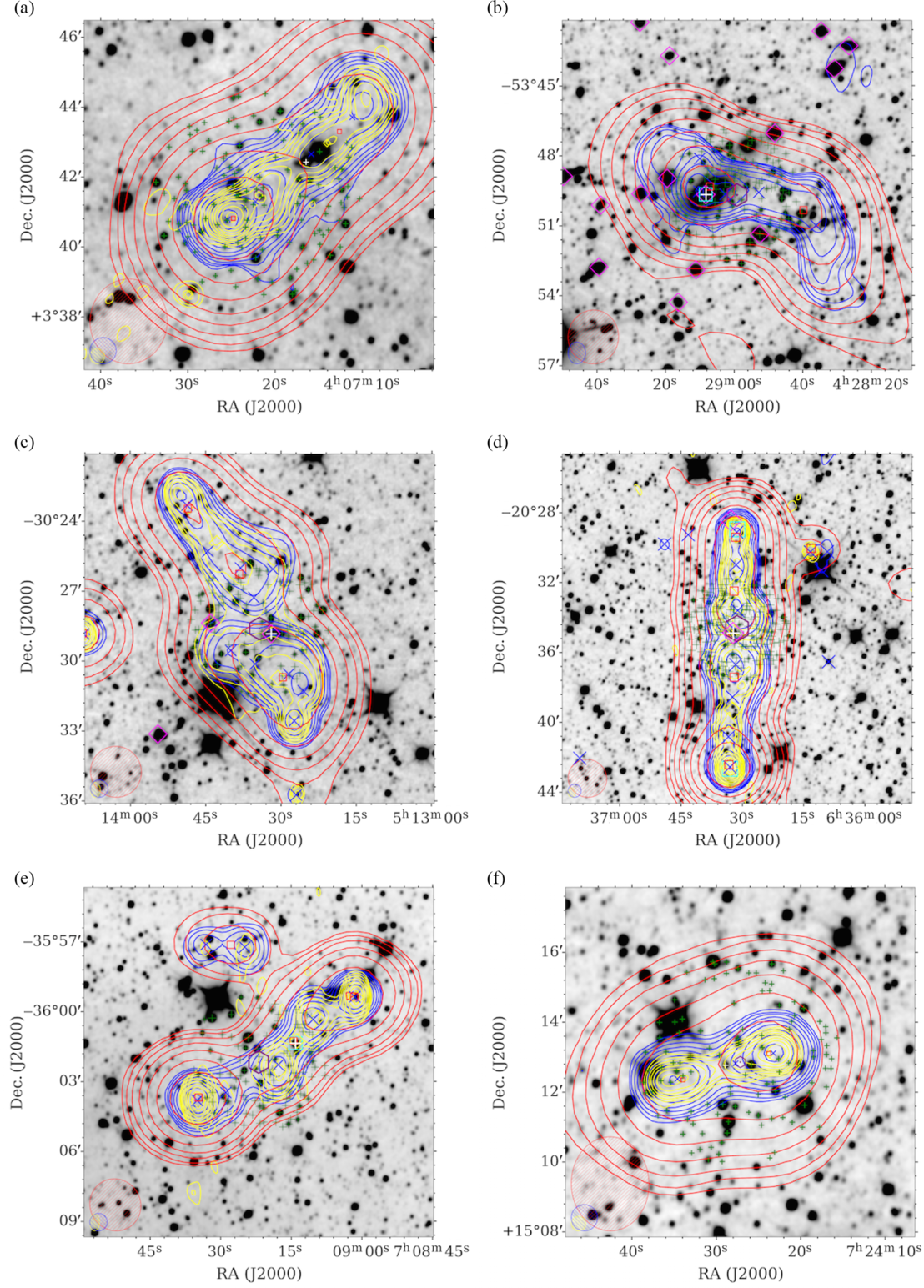
Figure C2. Overlays for G4Jy sources that have multiple GLEAM components (Table C1, Appendix C). The datasets, contours, symbols, and beams are the same as those used for Figure C1. (a) G4Jy 414. (b) G4Jy 462. (c) G4Jy 531. (d) G4Jy 619. (e) G4Jy 644. (f) G4Jy 659.
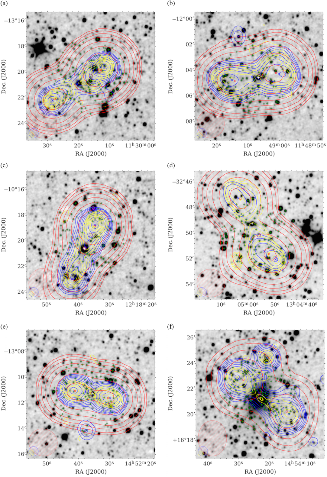
Figure C3. Overlays for G4Jy sources that have multiple GLEAM components (Table C1, Appendix C). The datasets, contours, symbols, and beams are the same as those used for Figure C1. (a) G4Jy 923. (b) G4Jy 957. (c) G4Jy 987. (d) G4Jy 1048. (e) G4Jy 1197. (f) G4Jy 1200.
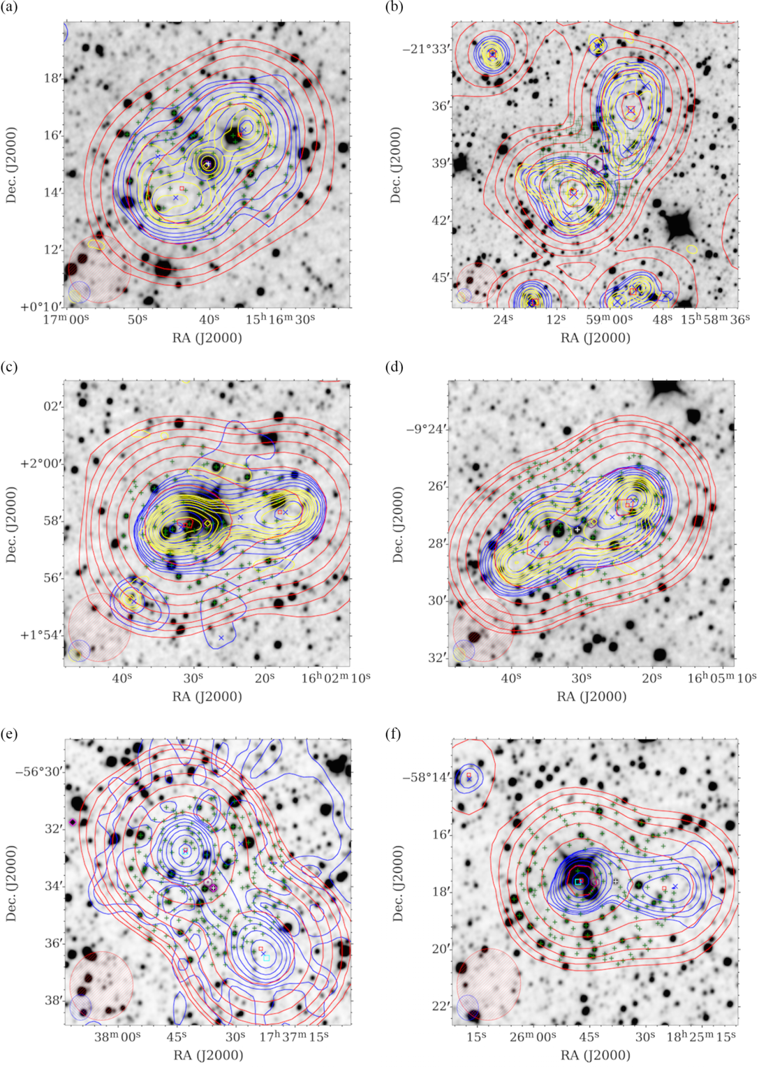
Figure C4. Overlays for G4Jy sources that have multiple GLEAM components (Table C1, Appendix C). The datasets, contours, symbols, and beams are the same as those used for Figure C1. (a) G4Jy 1238. (b) G4Jy 1289. (c) G4Jy 1296. (d) G4Jy 1303. (e) G4Jy 1423. (f) G4Jy 1484.
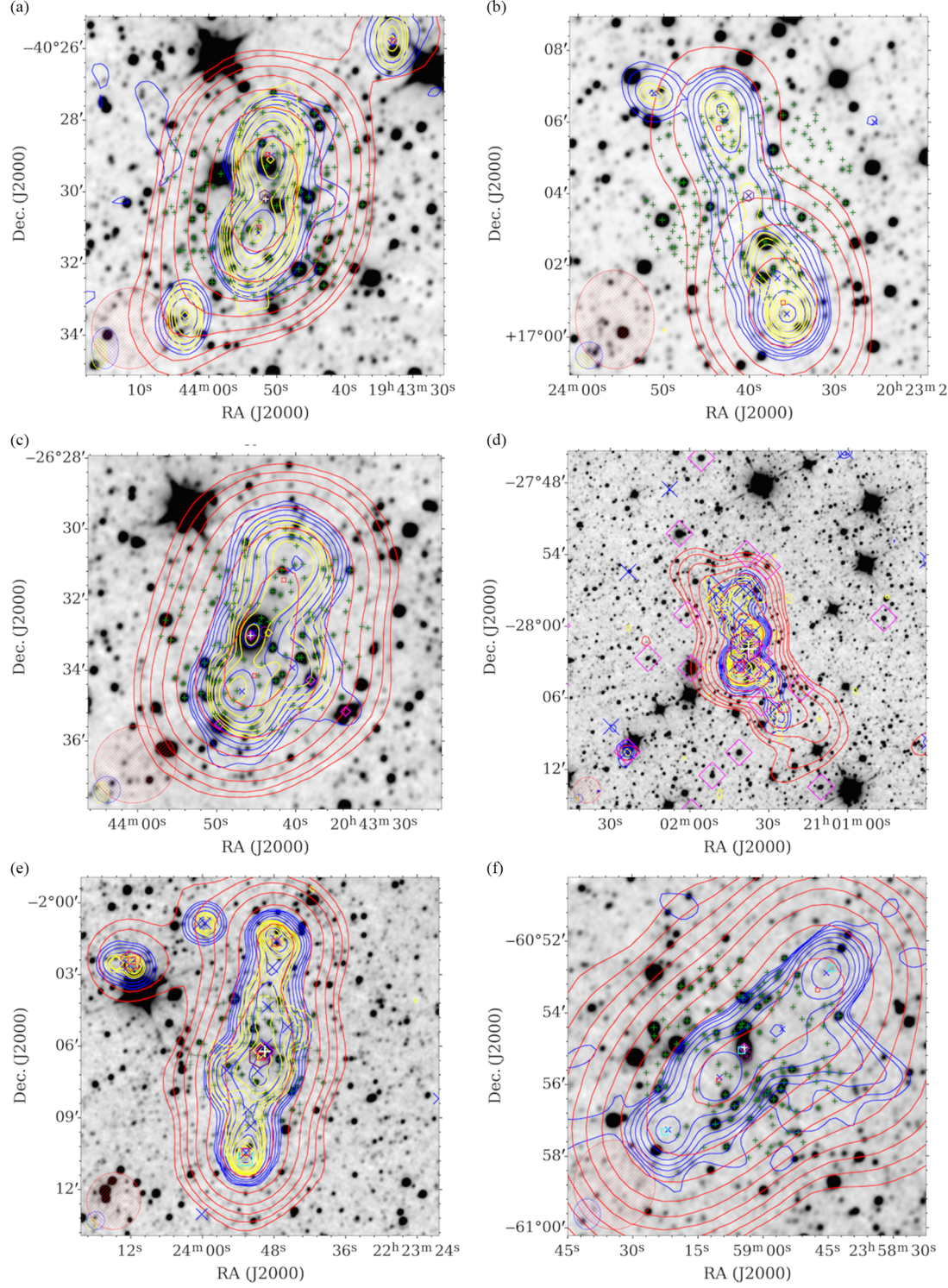
Figure C5. Overlays for G4Jy sources that have multiple GLEAM components (Table C1, Appendix C). The datasets, contours, symbols, and beams are the same as those used for Figure C1. (a) G4Jy 1569. (b) G4Jy 1617. (c) G4Jy 1643. (d) G4Jy 1671. (e) G4Jy 1775. (f) G4Jy 1863.
Table D1. Remeasured and fitted integrated flux densities for G4Jy 1558, which is PKS B1932 $-$
46 (Appendix D.2). To avoid extrapolating the SED-fit beyond the frequency range for which it is valid, we blank existing measurements in the G4Jy catalogue (Section 6) for the following sub-bands: 76, 84, 92, 99, and 227 MHz. The 200-MHz flux density and associated error correspond to the wide-band (170–231 MHz) measurement (replacing the original ‘int_flux_wide’ and ‘err_int_flux_wide’ values; see Appendix D). ‘Estimated’ refers to flux densities obtained via a fitted SED, rather than the application of a corrective flux scale factor (following reimaging).
$-$
46 (Appendix D.2). To avoid extrapolating the SED-fit beyond the frequency range for which it is valid, we blank existing measurements in the G4Jy catalogue (Section 6) for the following sub-bands: 76, 84, 92, 99, and 227 MHz. The 200-MHz flux density and associated error correspond to the wide-band (170–231 MHz) measurement (replacing the original ‘int_flux_wide’ and ‘err_int_flux_wide’ values; see Appendix D). ‘Estimated’ refers to flux densities obtained via a fitted SED, rather than the application of a corrective flux scale factor (following reimaging).
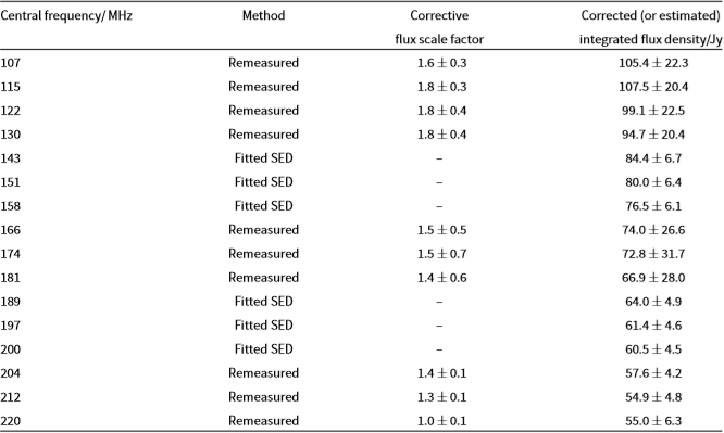
In the case of observations of PKSB1932 $-$
46 (G4Jy 1558), Cygnus A appeared in the far northern primary-beam sidelobe, with an apparent flux density that varied as a complex function of frequency. The automatic peeling algorithm attempted to remove Cygnus A, but at some sub-bands, the fitting converged on PKSB1932
$-$
46 (G4Jy 1558), Cygnus A appeared in the far northern primary-beam sidelobe, with an apparent flux density that varied as a complex function of frequency. The automatic peeling algorithm attempted to remove Cygnus A, but at some sub-bands, the fitting converged on PKSB1932 $-$
46, removing it from the images. When the images were mosaicked, PKSB1932–46 therefore had incorrect flux density measurements across the GLEAM band.
$-$
46, removing it from the images. When the images were mosaicked, PKSB1932–46 therefore had incorrect flux density measurements across the GLEAM band.
To correctly measure the SED, we reimaged five GLEAM observations covering PKSB1932 $-$
46, each covering 30.72 MHz of the GLEAM band in
$-$
46, each covering 30.72 MHz of the GLEAM band in  $4\times7.68$
MHz sub-bands, without applying any peeling. The lowest band (72–103 MHz) was found to be contaminated with RFI and was discarded. For the remaining 16 sub-bands, 10 were not affected by the presence of Cygnus A in the side lobes. From these, we were able to measure the flux density of PKSB1932
$4\times7.68$
MHz sub-bands, without applying any peeling. The lowest band (72–103 MHz) was found to be contaminated with RFI and was discarded. For the remaining 16 sub-bands, 10 were not affected by the presence of Cygnus A in the side lobes. From these, we were able to measure the flux density of PKSB1932 $-$
46, flux calibrate it to the 10 closest bright, isolated GLEAM sources, and fit an SED. Based on the fitted SED—a power-law function,
$-$
46, flux calibrate it to the 10 closest bright, isolated GLEAM sources, and fit an SED. Based on the fitted SED—a power-law function,  $S_{\nu} \propto \nu^{\alpha}$
, with
$S_{\nu} \propto \nu^{\alpha}$
, with  $\alpha = -1.0 \pm 0.1$
—we estimate the integrated flux density for the intervening, missing sub-band measurements. The G4Jy catalogue is updated to use these flux densities, which are provided in Table D1 for reference.
$\alpha = -1.0 \pm 0.1$
—we estimate the integrated flux density for the intervening, missing sub-band measurements. The G4Jy catalogue is updated to use these flux densities, which are provided in Table D1 for reference.
D.3. Priorised refitting
The morphology of the blended components GLEAM J213416 $-$
533648 and GLEAM J213356
$-$
533648 and GLEAM J213356 $-$
533524 is unclear (with the morphology of J21341775
$-$
533524 is unclear (with the morphology of J21341775 $-$
5338101 listed as ‘unknown’ by van Velzen et al. Reference van Velzen, Falcke, Schellart, NierstenhÖfer and Kampert2012). Using earlier Molonglo Observatory Synthesis Telescope observations at higher resolution, Jones & McAdam (Reference Jones and McAdam1992) interpreted the combined radio emission as arising from two double-lobed radio galaxies in the cluster A3785, confirming the optical identifications of Ekers (Reference Ekers1970). Follow-up ATCA observations at 1.34 GHz by Haigh (Reference Haigh2000)—published here for the first time—show clear evidence for relative motion, in opposite directions, between the host galaxies and the surrounding cluster gas (Figure D1). The radio structure of the northern galaxy, in particular, is not typical of a cluster radio source, as the jet between the core and the eastern lobe is well-collimated. This suggests that we might be witnessing the early(?) stages of a cluster merger, before the jet becomes disrupted.
$-$
5338101 listed as ‘unknown’ by van Velzen et al. Reference van Velzen, Falcke, Schellart, NierstenhÖfer and Kampert2012). Using earlier Molonglo Observatory Synthesis Telescope observations at higher resolution, Jones & McAdam (Reference Jones and McAdam1992) interpreted the combined radio emission as arising from two double-lobed radio galaxies in the cluster A3785, confirming the optical identifications of Ekers (Reference Ekers1970). Follow-up ATCA observations at 1.34 GHz by Haigh (Reference Haigh2000)—published here for the first time—show clear evidence for relative motion, in opposite directions, between the host galaxies and the surrounding cluster gas (Figure D1). The radio structure of the northern galaxy, in particular, is not typical of a cluster radio source, as the jet between the core and the eastern lobe is well-collimated. This suggests that we might be witnessing the early(?) stages of a cluster merger, before the jet becomes disrupted.
In an effort to de-blend the low-frequency emission from the two radio galaxies, we refit them using the SUMSS detections as priorised positions. Therefore, we replace the original two GLEAM components with GLEAM J213356 $-$
533509 and GLEAM J213418
$-$
533509 and GLEAM J213418 $-$
533514 (for the northern ‘double’), in addition to GLEAM J213415
$-$
533514 (for the northern ‘double’), in addition to GLEAM J213415 $-$
533736 and GLEAM J213422
$-$
533736 and GLEAM J213422 $-$
533756 (for the southern ‘double’). However, as a consequence of priorised fitting, the summation (per sub-band) of the resulting integrated flux densities (
$-$
533756 (for the southern ‘double’). However, as a consequence of priorised fitting, the summation (per sub-band) of the resulting integrated flux densities ( $\Sigma\,S_{\textrm{refitted}}$
) is systematically lower than the summation calculated for the original GLEAM components (
$\Sigma\,S_{\textrm{refitted}}$
) is systematically lower than the summation calculated for the original GLEAM components ( $\Sigma\,S_{\textrm{original}}$
). The ratio between these two sums is presented in Table D2 (under G4Jy 1704/G4Jy 1705) and shows that the proportion of low-frequency emission that is ‘recovered’ during the refitting is
$\Sigma\,S_{\textrm{original}}$
). The ratio between these two sums is presented in Table D2 (under G4Jy 1704/G4Jy 1705) and shows that the proportion of low-frequency emission that is ‘recovered’ during the refitting is  $>79\%$
. As we wish to provide the best estimate of integrated flux densities for these radio galaxies, we use the ratios to proportionally distribute
$>79\%$
. As we wish to provide the best estimate of integrated flux densities for these radio galaxies, we use the ratios to proportionally distribute  $\Sigma\,S_{\textrm{original}}$
across the refitted components. For example,
$\Sigma\,S_{\textrm{original}}$
across the refitted components. For example,
 \begin{equation}\begin{aligned}S_{\textrm{rescaled}}^{1} &= S_{\textrm{refitted}}^{1}\,\Sigma\,S_{\textrm{original}}\ /\ \Sigma\,S_{\textrm{refitted}} \\[3pt] &= \frac{S_{\textrm{refitted}}^{1}\,(S_{\textrm{original}}^{A} + S_{\textrm{original}}^{B})}{S_{\textrm{refitted}}^{1} + S_{\textrm{refitted}}^{2} + S_{\textrm{refitted}}^{3} + S_{\textrm{refitted}}^{4} },\end{aligned}\end{equation}
where superscripts are used to denote individual GLEAM components. We apply the same rescaling to the errors on the re-fitted, integrated flux densities.
Table D2. We present the ratio between the summed, integrated flux density for the refitted GLEAM components and the summed, integrated flux density for the original GLEAM components (i.e. ratio 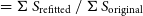 $= \Sigma\,S_{\textrm{refitted}}\ /\ \Sigma\,S_{\textrm{original}}$
). These ratios are calculated at each frequency for G4Jy 813, G4Jy 1410, and two sets of blended radio galaxies: G4Jy 1677/G4Jy 1678 and G4Jy 1704/G4Jy 1705. The ratios at 200 MHz correspond to the wide-band image (170–231 MHz). We use these ratios to correct integrated flux densities, which have been under-/overestimated as a result of priorised refitting (Appendix D.3).
$= \Sigma\,S_{\textrm{refitted}}\ /\ \Sigma\,S_{\textrm{original}}$
). These ratios are calculated at each frequency for G4Jy 813, G4Jy 1410, and two sets of blended radio galaxies: G4Jy 1677/G4Jy 1678 and G4Jy 1704/G4Jy 1705. The ratios at 200 MHz correspond to the wide-band image (170–231 MHz). We use these ratios to correct integrated flux densities, which have been under-/overestimated as a result of priorised refitting (Appendix D.3).

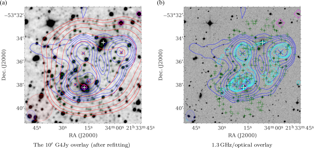
Figure D1. Two overlays for the radio galaxies (G4Jy 1704 and G4Jy 1705) in cluster Abell 3785. These sources required refitting with Aegean (Appendix D.3), with the new GLEAM positions (red squares) set to those of the SUMSS-catalogue positions (blue crosses), as shown in the first overlay, (a). Radio contours from GLEAM (170–231 MHz; red) and SUMSS (843 MHz; blue) are overlaid on a mid-infrared image from WISE (3.4 $\mu$
m; inverted greyscale). White plus signs indicate the host galaxies for the two G4Jy sources, whilst magenta diamonds represent 6dFGS positions. The second overlay, (b), uses an ATCA image at 1.3 GHz (cyan contours) from Haigh (Reference Haigh2000), which was provided courtesy of Richard Hunstead. This image was obtained using a combination of 6A and 6C configurations, with a restoring beam of 14.8 arcsec
$\mu$
m; inverted greyscale). White plus signs indicate the host galaxies for the two G4Jy sources, whilst magenta diamonds represent 6dFGS positions. The second overlay, (b), uses an ATCA image at 1.3 GHz (cyan contours) from Haigh (Reference Haigh2000), which was provided courtesy of Richard Hunstead. This image was obtained using a combination of 6A and 6C configurations, with a restoring beam of 14.8 arcsec  $\times$
9.6 arcsec at position angle =
$\times$
9.6 arcsec at position angle =  $-59^{\circ}$
(cyan ellipse in the bottom left-hand corner). The cyan contours are overlaid on an optical image (inverted greyscale) from SuperCOSMOS (Hambly et al. Reference Hambly2001), and SUMSS contours are again plotted in blue for reference. For each set of contours in this figure, the lowest contour is at the 3
$-59^{\circ}$
(cyan ellipse in the bottom left-hand corner). The cyan contours are overlaid on an optical image (inverted greyscale) from SuperCOSMOS (Hambly et al. Reference Hambly2001), and SUMSS contours are again plotted in blue for reference. For each set of contours in this figure, the lowest contour is at the 3 $\,\sigma$
level (where
$\,\sigma$
level (where  $\sigma$
is the local rms), with the number of
$\sigma$
is the local rms), with the number of  $\sigma$
doubling with each subsequent contour (i.e. 3, 6, 12
$\sigma$
doubling with each subsequent contour (i.e. 3, 6, 12 $\,\sigma$
, etc.).
$\,\sigma$
, etc.).
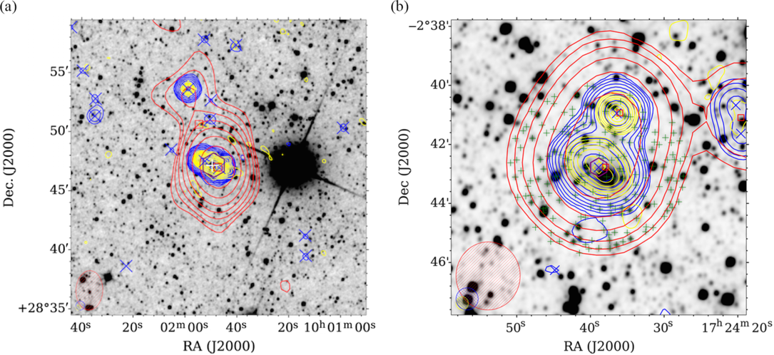
Figure D2. Overlays for (a) G4Jy 813 and (b) G4Jy 1410 (Appendix D.3), with the same datasets, contours, symbols, and beams as used for Figure 1. The red squares represent the original GLEAM positions for G4Jy 813 (shown for illustration), whilst for G4Jy 1410, they indicate the refitted GLEAM positions.
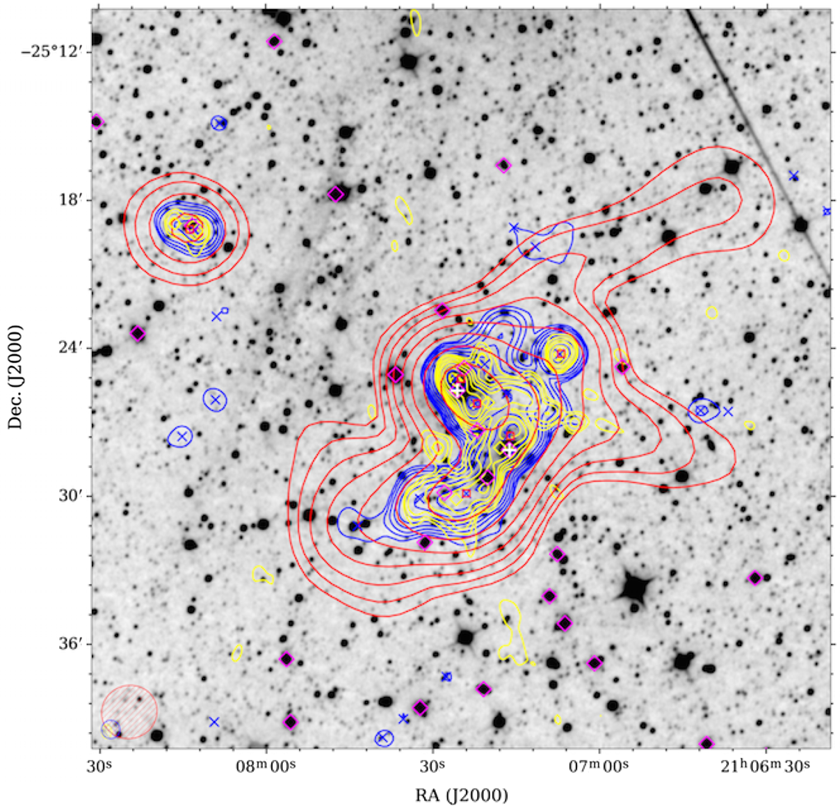
Figure D3. An overlay for G4Jy 1677 and G4Jy 1678 (Appendix D.3), with their host galaxies indicated by white plus signs (towards the west and east, respectively). Radio contours from TGSS (150 MHz; yellow), GLEAM (170–231 MHz; red), and NVSS (1.4 GHz; blue) are overlaid on a mid-infrared image from AllWISE ( $3.4\,\mu$
m; inverted greyscale). For each set of contours, the lowest contour is at the 3
$3.4\,\mu$
m; inverted greyscale). For each set of contours, the lowest contour is at the 3 $\,\sigma$
level (where
$\,\sigma$
level (where  $\sigma$
is the local rms), with the number of
$\sigma$
is the local rms), with the number of  $\sigma$
doubling with each subsequent contour (i.e. 3, 6, 12
$\sigma$
doubling with each subsequent contour (i.e. 3, 6, 12 $\,\sigma$
, etc.). Also plotted, in the bottom left-hand corner, are ellipses to indicate the beam sizes for TGSS (yellow with ‘+’ hatching), GLEAM (red with ‘/’ hatching), and NVSS (blue with ‘\’ hatching). Magenta diamonds represent optical positions for sources in 6dFGS, yellow diamonds represent TGSS positions, and blue crosses represent NVSS positions. Of the six GLEAM positions shown in this overlay (red squares), the five furthest west are following refitting with Aegean.
$\,\sigma$
, etc.). Also plotted, in the bottom left-hand corner, are ellipses to indicate the beam sizes for TGSS (yellow with ‘+’ hatching), GLEAM (red with ‘/’ hatching), and NVSS (blue with ‘\’ hatching). Magenta diamonds represent optical positions for sources in 6dFGS, yellow diamonds represent TGSS positions, and blue crosses represent NVSS positions. Of the six GLEAM positions shown in this overlay (red squares), the five furthest west are following refitting with Aegean.
Following this rescaling, we consider the summed flux density at 151 MHz for each of the radio galaxies. For the northern ‘double’ this is  $4.44 \pm 0.05\,\text{Jy}$
, and for the southern ‘double’ this is
$4.44 \pm 0.05\,\text{Jy}$
, and for the southern ‘double’ this is  $4.19 \pm 0.05\,\text{Jy}$
. As both radio galaxies cross the 4-Jy threshold, they are included in the G4Jy Sample (as G4Jy 1704 and G4Jy 1705, respectively). However, we emphasise that their integrated flux densities are estimates (rather than direct measurements), and note that they will be superseded by new measurements using the recently upgraded MWA (Beardsley et al. Reference Beardsley2019). This will provide higher spatial resolution (at
$4.19 \pm 0.05\,\text{Jy}$
. As both radio galaxies cross the 4-Jy threshold, they are included in the G4Jy Sample (as G4Jy 1704 and G4Jy 1705, respectively). However, we emphasise that their integrated flux densities are estimates (rather than direct measurements), and note that they will be superseded by new measurements using the recently upgraded MWA (Beardsley et al. Reference Beardsley2019). This will provide higher spatial resolution (at  $\sim1\textrm{arcmin}$
) than is currently available through GLEAM. For this reason, coupled with the involved process of refitting, we use the same method to de-blend only a few other confused sources in the sample.
$\sim1\textrm{arcmin}$
) than is currently available through GLEAM. For this reason, coupled with the involved process of refitting, we use the same method to de-blend only a few other confused sources in the sample.
Meanwhile, GLEAM J100154+285037 ( $S_{\textrm{151\,MHz}}=4.99 \pm 0.11 \,\text{Jy}$
) was found to be a poorly fitted component (Figure D2a) near to GLEAM J100147+284659 (G4Jy 813,
$S_{\textrm{151\,MHz}}=4.99 \pm 0.11 \,\text{Jy}$
) was found to be a poorly fitted component (Figure D2a) near to GLEAM J100147+284659 (G4Jy 813,  $S_{\textrm{151\,MHz}}=35.12 \pm 0.06\,\text{Jy}$
). This region was therefore refitted, with the positions of associated NVSS sources acting as priors. Again, the refitted components do not recover all of the low-frequency emission, as characterised by the original run of Aegean. Therefore we rescale the refitted, integrated flux densities (and their errors) using the ratios for G4Jy 813, given in Table D2. The result is GLEAM J100147+284659 now having
$S_{\textrm{151\,MHz}}=35.12 \pm 0.06\,\text{Jy}$
). This region was therefore refitted, with the positions of associated NVSS sources acting as priors. Again, the refitted components do not recover all of the low-frequency emission, as characterised by the original run of Aegean. Therefore we rescale the refitted, integrated flux densities (and their errors) using the ratios for G4Jy 813, given in Table D2. The result is GLEAM J100147+284659 now having  $S_{\textrm{151\,MHz}}=39.04 \pm 0.06\,\text{Jy}$
and GLEAM J100154+285037 being replaced with GLEAM J100159+285336 (
$S_{\textrm{151\,MHz}}=39.04 \pm 0.06\,\text{Jy}$
and GLEAM J100154+285037 being replaced with GLEAM J100159+285336 ( $S_{\textrm{151\,MHz}}=1.06 \pm 0.06 \,\text{Jy}$
). Since this new component is not above the 4-Jy threshold, it is not retained for this work.
$S_{\textrm{151\,MHz}}=1.06 \pm 0.06 \,\text{Jy}$
). Since this new component is not above the 4-Jy threshold, it is not retained for this work.
In the overlay for GLEAM J172438 $-$
024205 (
$-$
024205 ( $S_{\textrm{151\,MHz}}=9.54 \pm 0.07 \,\text{Jy}$
), we see that two unrelated sources have been blended together (Figure D2b). Using TGSS to determine whether either or both sources cross the 4-Jy threshold (see Section 5.2, and details for other GLEAM components in Appendix B), we find that the southern source (G4Jy 1410) is bright enough to be included in the G4Jy Sample. We proceed by refitting the low-frequency emission, using the two NVSS positions as priors. This gives rise to the GLEAM components, GLEAM J172436
$S_{\textrm{151\,MHz}}=9.54 \pm 0.07 \,\text{Jy}$
), we see that two unrelated sources have been blended together (Figure D2b). Using TGSS to determine whether either or both sources cross the 4-Jy threshold (see Section 5.2, and details for other GLEAM components in Appendix B), we find that the southern source (G4Jy 1410) is bright enough to be included in the G4Jy Sample. We proceed by refitting the low-frequency emission, using the two NVSS positions as priors. This gives rise to the GLEAM components, GLEAM J172436 $-$
024055 and GLEAM J172437
$-$
024055 and GLEAM J172437 $-$
024246. After applying the rescaling ratios calculated for G4Jy 1410 (Table D2), their integrated flux densities are
$-$
024246. After applying the rescaling ratios calculated for G4Jy 1410 (Table D2), their integrated flux densities are  $S_{\textrm{151\,MHz}}=3.79 \pm 0.07 \,\text{Jy}$
and
$S_{\textrm{151\,MHz}}=3.79 \pm 0.07 \,\text{Jy}$
and  $S_{\textrm{151\,MHz}}=5.74 \pm 0.07 \,\text{Jy}$
, respectively. We therefore remove GLEAM J172438
$S_{\textrm{151\,MHz}}=5.74 \pm 0.07 \,\text{Jy}$
, respectively. We therefore remove GLEAM J172438 $-$
024205 from the G4Jy Sample and replace it with GLEAM J172437
$-$
024205 from the G4Jy Sample and replace it with GLEAM J172437 $-$
024246.
$-$
024246.
Together, GLEAM J210722 $-$
252556 and GLEAM J210724
$-$
252556 and GLEAM J210724 $-$
252953 characterise the low-frequency emission of two ‘double’ radio galaxies and a single point source (Figure D3). In order to determine integrated flux densities for each source, separately, we again perform refitting. In this case, we set a total of five priorised positions: one for the point source, and one for each radio lobe belonging to the two doubles. Following rescaling (Table D2), the point source has a flux density below 4 Jy, and so is not considered any further. The southern double (GLEAM J210716-252733 and GLEAM J210724-252953) has total
$-$
252953 characterise the low-frequency emission of two ‘double’ radio galaxies and a single point source (Figure D3). In order to determine integrated flux densities for each source, separately, we again perform refitting. In this case, we set a total of five priorised positions: one for the point source, and one for each radio lobe belonging to the two doubles. Following rescaling (Table D2), the point source has a flux density below 4 Jy, and so is not considered any further. The southern double (GLEAM J210716-252733 and GLEAM J210724-252953) has total  $S_{\textrm{151\,MHz}}=18.56 \pm 0.05 \,\text{Jy}$
and becomes listed in the G4Jy Sample as G4Jy 1677. The northern double (GLEAM J210722
$S_{\textrm{151\,MHz}}=18.56 \pm 0.05 \,\text{Jy}$
and becomes listed in the G4Jy Sample as G4Jy 1677. The northern double (GLEAM J210722 $-$
252615 and GLEAM J210724
$-$
252615 and GLEAM J210724 $-$
252514) has total
$-$
252514) has total  $S_{\textrm{151\,MHz}}=23.19 \pm 0.05\,\text{Jy}$
and becomes listed in the G4Jy Sample as G4Jy 1678. Hence, the refitted, GLEAM components associated with these two double radio galaxies replace GLEAM J210722
$S_{\textrm{151\,MHz}}=23.19 \pm 0.05\,\text{Jy}$
and becomes listed in the G4Jy Sample as G4Jy 1678. Hence, the refitted, GLEAM components associated with these two double radio galaxies replace GLEAM J210722 $-$
252556 and GLEAM J210724
$-$
252556 and GLEAM J210724 $-$
252953 for the G4Jy catalogue.
$-$
252953 for the G4Jy catalogue.
E. Column descriptions and first row of the G4Jy catalogue
In Table E1, we list columns that are newly created for the G4Jy catalogue (Section 6), in addition to columns for wide-band (170–231 MHz) and 151-MHz measurements, inherited from the EGC (Hurley-Walker et al. Reference Hurley-Walker2017). Equivalent columns for the remaining GLEAM sub-bands (76, 84, 92, 99, 107, 115, 122, 130, 143, 158, 166, 174, 181, 189, 197, 204, 212, 220, and 227 MHz) are listed in Appendix A of Hurley-Walker et al. (Reference Hurley-Walker2017). Example entries, for the first row of the G4Jy catalogue, are also provided in Table E1.
F. Broadband radio spectra for G4Jy–3CRR sources
As part of our comparison with the 3CRR sample (Section 7.3), we plot summed, GLEAM integrated flux densities alongside measurements obtained for 3CR sources, spanning 10 MHz to 15 GHz (Laing & Peacock Reference Laing and Peacock1980). We thank Robert Laing for providing a compilation of the latter. Note that this does not include data for the following sources: G4Jy 18 (4C +12.03), G4Jy 432 (4C +14.11), G4Jy 714 (4C +14.27), G4Jy 1004 (1227+119), G4Jy 1282 (3C 326), G4Jy 1419 (4C +16.49), and G4Jy 1456 (4C+ 13.66). This is because these sources were added later, during the creation of the 3CRR sample (Laing et al. Reference Laing, Riley and Longair1983), or—in the case of 3C 326—the source was omitted by Laing & Peacock (Reference Laing and Peacock1980) because its ‘integrated flux densities are not well known’. These spectra are available online as supplementary material.
Table E1. Column numbers, names, units, descriptions, and first-row entries for 117 of the 383 columns in the G4Jy catalogue (Section 6, Appendix E). Mid-infrared information is taken from the AllWISE catalogue (Cutri et al. Reference Cutri2013), and ‘PSF’ stands for ‘point spread function’. See appendix A of Hurley-Walker et al. (Reference Hurley-Walker2017) for the remaining 266 G4Jy-catalogue columns.
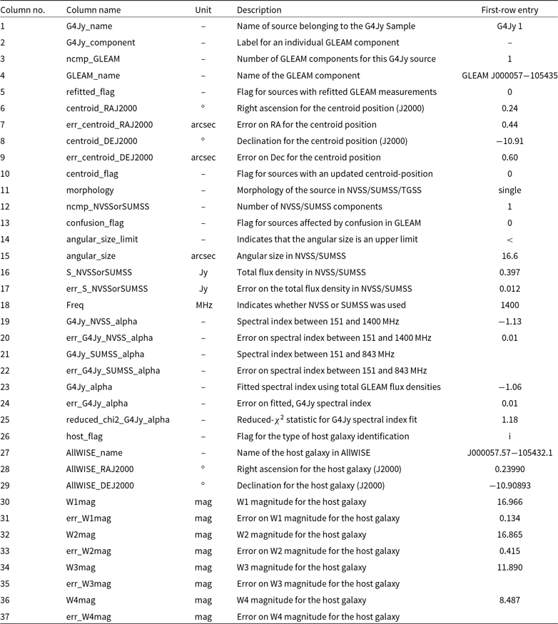
Table E1. Continued - Column numbers, names, units, descriptions, and first-row entries for 117 of the 383 columns in the G4Jy catalogue (Section 6, Appendix E).
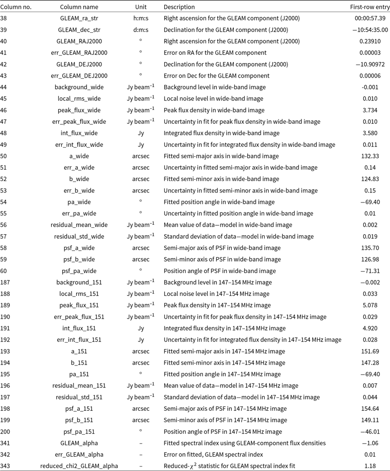
Table E1. Continued - Column numbers, names, units, descriptions, and first-row entries for 117 of the 383 columns in the G4Jy catalogue (Section 6, Appendix E).